Exponential Function
1. Introduction to Exponential Functions
Learning outcomes
- I can define an exponential function.
- I can distinguish exponential functions from linear and polynomial functions.
- I can identify the components of an exponential equation.
- I can evaluate exponential functions.
- I can recognise exponential relationships in real-world situations.
Introduction
Some quantities change by repeatedly adding the same amount. For example, a water tank filled at a rate of 5 litres per minute increases by a constant amount. This type of change can be represented by a linear function.
Other quantities change by repeatedly multiplying by the same factor. A population might double every year, an investment might increase by 5% annually, or the amount of a medicine in the bloodstream might decrease by 20% every hour. These relationships can be represented by exponential functions.
Exponential functions are used to model population growth, compound interest, depreciation, radioactive decay, repeated cell division, and many other real-world processes.
What Is an Exponential Function?
An exponential function is a function in which the independent variable appears in the exponent.
The general form is:
f(x) = a(bˣ)
It may also be written as:
y = a(bˣ)
For a standard exponential function:
- a cannot equal 0.
- b must be greater than 0.
- b cannot equal 1.
- x is the independent variable.
Consider the example:
f(x) = 3(2ˣ)
As x increases by 1, the output is multiplied by 2.
| x | f(x) = 3(2ˣ) |
|---|---|
| 0 | 3 |
| 1 | 6 |
| 2 | 12 |
| 3 | 24 |
| 4 | 48 |
The outputs do not increase by the same amount. Instead, each output is twice the previous output.
Components of an Exponential Function
Consider the general form:
f(x) = a(bˣ)
Each component has a particular meaning.
The Initial Value: a
The value of a represents the initial value. It is the value of the function when x = 0.
This is because any non-zero number raised to the power of zero equals 1:
b⁰ = 1
Therefore:
f(0) = a(b⁰)
f(0) = a(1)
f(0) = a
For example:
f(x) = 5(3ˣ)
When x = 0:
f(0) = 5(3⁰)
f(0) = 5(1)
f(0) = 5
The initial value is 5. The graph crosses the y-axis at the point (0, 5).
The Base: b
The value of b is the base of the exponential expression. It determines how quickly the function grows or decays.
The base may also be called the:
- Growth factor, when b > 1.
- Decay factor, when 0 < b < 1.
For example:
f(x) = 4(2ˣ)
The base is 2. Each time x increases by 1, the output is multiplied by 2.
In another function:
f(x) = 100(0.5ˣ)
The base is 0.5. Each time x increases by 1, the output is multiplied by 0.5.
The Exponent: x
The variable x appears in the exponent. It represents the input or the number of intervals that have passed.
Depending on the situation, x might represent:
- Time in seconds.
- Time in years.
- Number of reproduction cycles.
- Number of interest periods.
- Number of repeated multiplications.
- Number of half-lives.
The Output: f(x)
The value f(x) is the output produced by the function.
In a real-world model, f(x) might represent:
- The size of a population.
- The value of an investment.
- The number of bacterial cells.
- The remaining mass of a radioactive substance.
- The value of a depreciating vehicle.
Exponential Growth
An exponential function represents exponential growth when its base is greater than 1.
General form:
f(x) = a(bˣ), where b > 1
For example:
f(x) = 200(1.4ˣ)
The initial value is 200, and the growth factor is 1.4. Each time x increases by 1, the output is multiplied by 1.4.
This represents a 40% increase during each interval because:
1.4 = 1 + 0.4
The decimal 0.4 is equivalent to 40%.
The growth factor for a percentage increase is:
Growth factor = 1 + growth rate
The growth rate must be written as a decimal.
Examples include:
- A 5% increase has a growth factor of 1.05.
- A 12% increase has a growth factor of 1.12.
- A 25% increase has a growth factor of 1.25.
- A 100% increase has a growth factor of 2.
Exponential Decay
An exponential function represents exponential decay when its base is between 0 and 1.
General form:
f(x) = a(bˣ), where 0 < b < 1
For example:
f(x) = 500(0.8ˣ)
The initial value is 500, and the decay factor is 0.8. Each time x increases by 1, 80% of the previous amount remains.
This represents a decrease of 20% because:
1 − 0.8 = 0.2
The decimal 0.2 is equivalent to 20%.
The decay factor for a percentage decrease is:
Decay factor = 1 − decay rate
Examples include:
- A 5% decrease has a decay factor of 0.95.
- A 10% decrease has a decay factor of 0.90.
- A 25% decrease has a decay factor of 0.75.
- A 50% decrease has a decay factor of 0.50.
Exponential, Linear, and Polynomial Functions
The position of the variable helps identify the type of function.
Linear Functions
A linear function has a constant additive rate of change.
General form:
f(x) = mx + c
Example:
f(x) = 3x + 2
Each time x increases by 1, the output increases by 3.
A linear function has:
- A constant first difference.
- A straight-line graph.
- A variable raised to the first power.
Polynomial Functions
A polynomial function contains variables raised to fixed non-negative whole-number exponents.
Examples include:
f(x) = x² + 3x − 4
f(x) = 2x³ − 5x
In x³:
- x is the base.
- 3 is a fixed exponent.
Exponential Functions
An exponential function has the independent variable in the exponent.
Example:
f(x) = 3(2ˣ)
In this expression:
- 2 is the base.
- x is the exponent.
Exponential functions change through repeated multiplication rather than repeated addition.
How to Identify an Exponential Function
Consider these three functions:
- f(x) = 4x + 3
- f(x) = 4x² + 3
- f(x) = 4(2ˣ) + 3
The first function is linear because x is raised to the first power.
The second function is polynomial because x is the base and 2 is a fixed exponent.
The third function is exponential because x appears in the exponent.
Examples of Exponential Functions
- y = 2ˣ
- y = 5(3ˣ)
- y = 100(0.9ˣ)
- y = 7(1.25ˣ)
- y = 4ˣ + 6
Examples That Are Not Exponential Functions
- y = 2x + 5 is linear.
- y = x² is quadratic.
- y = 3x⁴ − 2x is polynomial.
- y = 1/x is rational.
- y = √x is a radical function.
Recognising Exponential Relationships in Tables
An exponential relationship has a constant multiplicative rate of change.
Consider the following table:
| x | y |
|---|---|
| 0 | 3 |
| 1 | 6 |
| 2 | 12 |
| 3 | 24 |
| 4 | 48 |
Divide each output by the previous output:
6 ÷ 3 = 2
12 ÷ 6 = 2
24 ÷ 12 = 2
48 ÷ 24 = 2
The ratio is always 2. Therefore, the relationship is exponential.
The equation is:
y = 3(2ˣ)
The initial value is 3, and the growth factor is 2.
Comparing Linear and Exponential Tables
A linear pattern has constant differences.
| x | Linear output |
|---|---|
| 0 | 3 |
| 1 | 6 |
| 2 | 9 |
| 3 | 12 |
| 4 | 15 |
The outputs increase by 3 each time.
An exponential pattern has constant ratios.
| x | Exponential output |
|---|---|
| 0 | 3 |
| 1 | 6 |
| 2 | 12 |
| 3 | 24 |
| 4 | 48 |
The outputs are multiplied by 2 each time.
The important distinction is:
- Constant difference indicates a linear relationship.
- Constant ratio indicates an exponential relationship.
Evaluating Exponential Functions
To evaluate a function, substitute the given input and calculate the output.
Always calculate the exponent before multiplying by the initial value.
Worked Example 1
Evaluate f(x) = 3(2ˣ) when x = 4.
Substitute x = 4:
f(4) = 3(2⁴)
Calculate the exponent:
f(4) = 3(16)
Multiply:
f(4) = 48
Therefore, f(4) = 48.
Worked Example 2
Evaluate f(x) = 200(0.5ˣ) when x = 3.
Substitute x = 3:
f(3) = 200(0.5³)
Calculate the exponent:
f(3) = 200(0.125)
Multiply:
f(3) = 25
Therefore, f(3) = 25.
Worked Example 3
Evaluate g(t) = 80(1.2ᵗ) when t = 2.
Substitute t = 2:
g(2) = 80(1.2²)
Calculate the exponent:
g(2) = 80(1.44)
Multiply:
g(2) = 115.2
Therefore, g(2) = 115.2.
Worked Example 4: Zero Exponent
Evaluate h(x) = 12(4ˣ) when x = 0.
h(0) = 12(4⁰)
h(0) = 12(1)
h(0) = 12
This confirms that 12 is the initial value.
Worked Example 5: Negative Exponent
Evaluate f(x) = 8(2ˣ) when x = −2.
f(−2) = 8(2⁻²)
A negative exponent represents a reciprocal:
2⁻² = 1/2² = 1/4
Therefore:
f(−2) = 8(1/4)
f(−2) = 2
Basic Features of Exponential Graphs
The graph of an exponential function is curved rather than straight.
For the basic function f(x) = a(bˣ), where a is positive:
- The y-intercept is (0, a).
- The domain is all real numbers.
- The range is y > 0.
- The outputs remain positive.
- The graph approaches the x-axis but does not touch it.
- The horizontal line y = 0 is an asymptote.
- A base greater than 1 produces an increasing graph.
- A base between 0 and 1 produces a decreasing graph.
An asymptote is a line that a graph approaches increasingly closely.
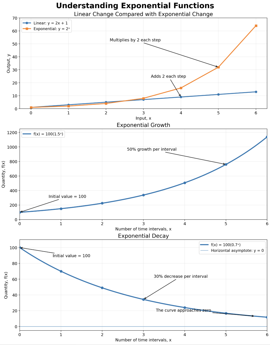
The first graph shows that a linear function adds the same amount during each interval, while an exponential function multiplies by the same factor.
The growth graph curves upwards because the amount added becomes progressively larger. The decay graph curves downwards and approaches zero because only a fraction of the previous amount remains after each interval.
Real-World Exponential Relationships
Exponential models are useful when a quantity changes by the same factor or percentage during equal intervals.
Population Growth
Suppose a population begins with 500 organisms and increases by 10% each year.
The growth factor is:
1 + 0.10 = 1.10
The model is:
P(t) = 500(1.10ᵗ)
In this model:
- P(t) is the population after t years.
- 500 is the initial population.
- 1.10 is the annual growth factor.
- t is the number of years.
After three years:
P(3) = 500(1.10³)
P(3) = 500(1.331)
P(3) = 665.5
The model predicts a population of approximately 666 organisms.
Repeated Cell Division
Suppose one bacterial cell divides into two cells every 20 minutes. If every cell continues dividing, the number of cells follows this pattern:
| Number of divisions | Number of cells |
|---|---|
| 0 | 1 |
| 1 | 2 |
| 2 | 4 |
| 3 | 8 |
| 4 | 16 |
| 5 | 32 |
The equation is:
N(d) = 2ᵈ
The number of cells doubles during each division cycle.


Compound Interest
Money in an investment account may increase by the same percentage each year. Interest is added to the balance, and future interest is calculated using the new balance.
Suppose $1,000 is invested at an annual interest rate of 4%.
The growth factor is:
1 + 0.04 = 1.04
The model is:
A(t) = 1000(1.04ᵗ)
After five years:
A(5) = 1000(1.04⁵)
A(5) ≈ 1216.65
The investment would be worth approximately $1,216.65.
Depreciation
Many objects lose a percentage of their value each year.
Suppose a computer is initially worth $1,500 and loses 20% of its value annually.
The decay factor is:
1 − 0.20 = 0.80
The model is:
V(t) = 1500(0.80ᵗ)
After three years:
V(3) = 1500(0.80³)
V(3) = 1500(0.512)
V(3) = 768
The computer would be worth approximately $768.
Radioactive Decay
Radioactive substances decay by losing the same fraction of their unstable nuclei during equal intervals.
If a sample has a half-life of 10 years, half of the radioactive material remains after every 10-year interval.
A model could be written as:
M = M₀(0.5ⁿ)
In this model:
- M
is the remaining mass.
- M₀ is the initial mass.
- 0.5 is the decay factor.
- n is the number of half-life intervals.
How to Decide Whether a Situation Is Exponential
Ask the following questions:
- Is the quantity changing by the same percentage during equal intervals?
- Is the quantity being multiplied by the same factor repeatedly?
- Do the outputs have a constant ratio?
- Does the variable represent the number of repeated periods or cycles?
- Does the variable appear in the exponent?
If the answer to these questions is yes, an exponential model may be appropriate.
A relationship is not exponential simply because it increases quickly. Its defining feature is repeated multiplication by the same factor over equal intervals.
Common Misconceptions
Any Rapidly Increasing Function Is Exponential
A quadratic or cubic function may increase rapidly, but it is not exponential unless the variable appears in the exponent.
The Base and Exponent Can Be Exchanged
The expressions 2ˣ and x² represent different types of functions.
- 2ˣ is exponential because x is the exponent.
- x² is polynomial because x is the base.
Exponential Growth Adds the Same Amount Each Time
Exponential growth multiplies by the same factor. The amount added changes during each interval.
A Decay Factor of 0.8 Means an 80% Decrease
A decay factor of 0.8 means that 80% remains. Therefore, the quantity decreases by 20%.
The Initial Value Occurs When x = 1
The initial value occurs when x = 0 because b⁰ = 1.
Real-World Connections
Exponential functions are used in many areas:
- Biologists model population growth.
- Epidemiologists study the early spread of infectious diseases.
- Physicists model radioactive decay.
- Pharmacologists model the removal of medicines from the body.
- Financial institutions calculate compound interest.
- Businesses estimate depreciation.
- Computer scientists analyse repeated doubling and data growth.
- Environmental scientists model changes in populations and resources.
Exponential models are most reliable when the growth or decay factor remains approximately constant. Environmental limits, resource shortages, changing interest rates, and human actions can cause real patterns to differ from a simple exponential model.
Did You Know?
Exponential growth can begin slowly and then become extremely rapid.
If a quantity doubles repeatedly, it becomes 1,024 times its original size after only ten doublings:
2¹⁰ = 1,024
After twenty doublings:
2²⁰ = 1,048,576
This rapid increase explains why exponential growth can be difficult to recognise during its early stages.
Key Terms
- Asymptote: A line that a graph approaches increasingly closely.
- Base: The number that is repeatedly multiplied in an exponential expression.
- Constant difference: A pattern in which the same amount is added or subtracted between consecutive outputs.
- Constant ratio: A pattern in which consecutive outputs are multiplied or divided by the same factor.
- Decay factor: A number between 0 and 1 by which a quantity is multiplied during each interval.
- Dependent variable: The output whose value depends on the input.
- Domain: The complete set of possible input values for a function.
- Evaluate: To calculate the output of a function for a particular input.
- Exponent: A number or variable showing how many times a base is used as a factor.
- Exponential decay: A pattern in which a quantity decreases by the same factor or percentage during equal intervals.
- Exponential function: A function in which the independent variable appears in the exponent.
- Exponential growth: A pattern in which a quantity increases by the same factor or percentage during equal intervals.
- Function: A relationship that assigns exactly one output to each permitted input.
- Growth factor: A number greater than 1 by which a quantity is multiplied during each interval.
- Growth rate: The percentage or decimal rate by which a quantity increases.
- Half-life: The time required for half of a radioactive substance to decay.
- Independent variable: The input that is selected or changed.
- Initial value: The value of an exponential function when the input is zero.
- Linear function: A function with a constant additive rate of change and a straight-line graph.
- Polynomial function: A function containing variables raised to fixed non-negative whole-number powers.
- Range: The complete set of possible output values for a function.
- y-intercept: The point where a graph crosses the y-axis. For f(x) = a(bˣ), it is (0, a).
Key Takeaways
- An exponential function has the independent variable in the exponent.
- The general form is f(x) = a(bˣ).
- The value a is the initial value and determines the y-intercept.
- The value b is the growth or decay factor.
- A base greater than 1 represents exponential growth.
- A base between 0 and 1 represents exponential decay.
- Linear functions have constant differences.
- Exponential functions have constant ratios.
- Polynomial functions have variables raised to fixed whole-number exponents.
- Exponential functions are evaluated by calculating the exponent before multiplying.
- Exponential growth curves upwards and becomes increasingly steep.
- Exponential decay curves downwards and approaches a horizontal asymptote.
- Population growth, compound interest, depreciation, radioactive decay, and repeated cell division can all be modelled using exponential functions.