Exponential Function
| Сайт: | Young Education |
| Курс: | Exponential and Logarithmic Functions |
| Книга: | Exponential Function |
| Надруковано: | Guest user |
| Дата: | понеділок 9 листопада 2026 16:39 PM |
1. Introduction to Exponential Functions
Learning outcomes
- I can define an exponential function.
- I can distinguish exponential functions from linear and polynomial functions.
- I can identify the components of an exponential equation.
- I can evaluate exponential functions.
- I can recognise exponential relationships in real-world situations.
Introduction
Some quantities change by repeatedly adding the same amount. For example, a water tank filled at a rate of 5 litres per minute increases by a constant amount. This type of change can be represented by a linear function.
Other quantities change by repeatedly multiplying by the same factor. A population might double every year, an investment might increase by 5% annually, or the amount of a medicine in the bloodstream might decrease by 20% every hour. These relationships can be represented by exponential functions.
Exponential functions are used to model population growth, compound interest, depreciation, radioactive decay, repeated cell division, and many other real-world processes.
What Is an Exponential Function?
An exponential function is a function in which the independent variable appears in the exponent.
The general form is:
f(x) = a(bˣ)
It may also be written as:
y = a(bˣ)
For a standard exponential function:
- a cannot equal 0.
- b must be greater than 0.
- b cannot equal 1.
- x is the independent variable.
Consider the example:
f(x) = 3(2ˣ)
As x increases by 1, the output is multiplied by 2.
| x | f(x) = 3(2ˣ) |
|---|---|
| 0 | 3 |
| 1 | 6 |
| 2 | 12 |
| 3 | 24 |
| 4 | 48 |
The outputs do not increase by the same amount. Instead, each output is twice the previous output.
Components of an Exponential Function
Consider the general form:
f(x) = a(bˣ)
Each component has a particular meaning.
The Initial Value: a
The value of a represents the initial value. It is the value of the function when x = 0.
This is because any non-zero number raised to the power of zero equals 1:
b⁰ = 1
Therefore:
f(0) = a(b⁰)
f(0) = a(1)
f(0) = a
For example:
f(x) = 5(3ˣ)
When x = 0:
f(0) = 5(3⁰)
f(0) = 5(1)
f(0) = 5
The initial value is 5. The graph crosses the y-axis at the point (0, 5).
The Base: b
The value of b is the base of the exponential expression. It determines how quickly the function grows or decays.
The base may also be called the:
- Growth factor, when b > 1.
- Decay factor, when 0 < b < 1.
For example:
f(x) = 4(2ˣ)
The base is 2. Each time x increases by 1, the output is multiplied by 2.
In another function:
f(x) = 100(0.5ˣ)
The base is 0.5. Each time x increases by 1, the output is multiplied by 0.5.
The Exponent: x
The variable x appears in the exponent. It represents the input or the number of intervals that have passed.
Depending on the situation, x might represent:
- Time in seconds.
- Time in years.
- Number of reproduction cycles.
- Number of interest periods.
- Number of repeated multiplications.
- Number of half-lives.
The Output: f(x)
The value f(x) is the output produced by the function.
In a real-world model, f(x) might represent:
- The size of a population.
- The value of an investment.
- The number of bacterial cells.
- The remaining mass of a radioactive substance.
- The value of a depreciating vehicle.
Exponential Growth
An exponential function represents exponential growth when its base is greater than 1.
General form:
f(x) = a(bˣ), where b > 1
For example:
f(x) = 200(1.4ˣ)
The initial value is 200, and the growth factor is 1.4. Each time x increases by 1, the output is multiplied by 1.4.
This represents a 40% increase during each interval because:
1.4 = 1 + 0.4
The decimal 0.4 is equivalent to 40%.
The growth factor for a percentage increase is:
Growth factor = 1 + growth rate
The growth rate must be written as a decimal.
Examples include:
- A 5% increase has a growth factor of 1.05.
- A 12% increase has a growth factor of 1.12.
- A 25% increase has a growth factor of 1.25.
- A 100% increase has a growth factor of 2.
Exponential Decay
An exponential function represents exponential decay when its base is between 0 and 1.
General form:
f(x) = a(bˣ), where 0 < b < 1
For example:
f(x) = 500(0.8ˣ)
The initial value is 500, and the decay factor is 0.8. Each time x increases by 1, 80% of the previous amount remains.
This represents a decrease of 20% because:
1 − 0.8 = 0.2
The decimal 0.2 is equivalent to 20%.
The decay factor for a percentage decrease is:
Decay factor = 1 − decay rate
Examples include:
- A 5% decrease has a decay factor of 0.95.
- A 10% decrease has a decay factor of 0.90.
- A 25% decrease has a decay factor of 0.75.
- A 50% decrease has a decay factor of 0.50.
Exponential, Linear, and Polynomial Functions
The position of the variable helps identify the type of function.
Linear Functions
A linear function has a constant additive rate of change.
General form:
f(x) = mx + c
Example:
f(x) = 3x + 2
Each time x increases by 1, the output increases by 3.
A linear function has:
- A constant first difference.
- A straight-line graph.
- A variable raised to the first power.
Polynomial Functions
A polynomial function contains variables raised to fixed non-negative whole-number exponents.
Examples include:
f(x) = x² + 3x − 4
f(x) = 2x³ − 5x
In x³:
- x is the base.
- 3 is a fixed exponent.
Exponential Functions
An exponential function has the independent variable in the exponent.
Example:
f(x) = 3(2ˣ)
In this expression:
- 2 is the base.
- x is the exponent.
Exponential functions change through repeated multiplication rather than repeated addition.
How to Identify an Exponential Function
Consider these three functions:
- f(x) = 4x + 3
- f(x) = 4x² + 3
- f(x) = 4(2ˣ) + 3
The first function is linear because x is raised to the first power.
The second function is polynomial because x is the base and 2 is a fixed exponent.
The third function is exponential because x appears in the exponent.
Examples of Exponential Functions
- y = 2ˣ
- y = 5(3ˣ)
- y = 100(0.9ˣ)
- y = 7(1.25ˣ)
- y = 4ˣ + 6
Examples That Are Not Exponential Functions
- y = 2x + 5 is linear.
- y = x² is quadratic.
- y = 3x⁴ − 2x is polynomial.
- y = 1/x is rational.
- y = √x is a radical function.
Recognising Exponential Relationships in Tables
An exponential relationship has a constant multiplicative rate of change.
Consider the following table:
| x | y |
|---|---|
| 0 | 3 |
| 1 | 6 |
| 2 | 12 |
| 3 | 24 |
| 4 | 48 |
Divide each output by the previous output:
6 ÷ 3 = 2
12 ÷ 6 = 2
24 ÷ 12 = 2
48 ÷ 24 = 2
The ratio is always 2. Therefore, the relationship is exponential.
The equation is:
y = 3(2ˣ)
The initial value is 3, and the growth factor is 2.
Comparing Linear and Exponential Tables
A linear pattern has constant differences.
| x | Linear output |
|---|---|
| 0 | 3 |
| 1 | 6 |
| 2 | 9 |
| 3 | 12 |
| 4 | 15 |
The outputs increase by 3 each time.
An exponential pattern has constant ratios.
| x | Exponential output |
|---|---|
| 0 | 3 |
| 1 | 6 |
| 2 | 12 |
| 3 | 24 |
| 4 | 48 |
The outputs are multiplied by 2 each time.
The important distinction is:
- Constant difference indicates a linear relationship.
- Constant ratio indicates an exponential relationship.
Evaluating Exponential Functions
To evaluate a function, substitute the given input and calculate the output.
Always calculate the exponent before multiplying by the initial value.
Worked Example 1
Evaluate f(x) = 3(2ˣ) when x = 4.
Substitute x = 4:
f(4) = 3(2⁴)
Calculate the exponent:
f(4) = 3(16)
Multiply:
f(4) = 48
Therefore, f(4) = 48.
Worked Example 2
Evaluate f(x) = 200(0.5ˣ) when x = 3.
Substitute x = 3:
f(3) = 200(0.5³)
Calculate the exponent:
f(3) = 200(0.125)
Multiply:
f(3) = 25
Therefore, f(3) = 25.
Worked Example 3
Evaluate g(t) = 80(1.2ᵗ) when t = 2.
Substitute t = 2:
g(2) = 80(1.2²)
Calculate the exponent:
g(2) = 80(1.44)
Multiply:
g(2) = 115.2
Therefore, g(2) = 115.2.
Worked Example 4: Zero Exponent
Evaluate h(x) = 12(4ˣ) when x = 0.
h(0) = 12(4⁰)
h(0) = 12(1)
h(0) = 12
This confirms that 12 is the initial value.
Worked Example 5: Negative Exponent
Evaluate f(x) = 8(2ˣ) when x = −2.
f(−2) = 8(2⁻²)
A negative exponent represents a reciprocal:
2⁻² = 1/2² = 1/4
Therefore:
f(−2) = 8(1/4)
f(−2) = 2
Basic Features of Exponential Graphs
The graph of an exponential function is curved rather than straight.
For the basic function f(x) = a(bˣ), where a is positive:
- The y-intercept is (0, a).
- The domain is all real numbers.
- The range is y > 0.
- The outputs remain positive.
- The graph approaches the x-axis but does not touch it.
- The horizontal line y = 0 is an asymptote.
- A base greater than 1 produces an increasing graph.
- A base between 0 and 1 produces a decreasing graph.
An asymptote is a line that a graph approaches increasingly closely.
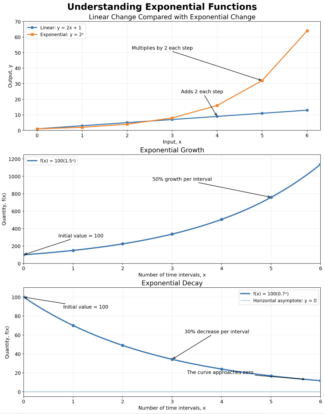
The first graph shows that a linear function adds the same amount during each interval, while an exponential function multiplies by the same factor.
The growth graph curves upwards because the amount added becomes progressively larger. The decay graph curves downwards and approaches zero because only a fraction of the previous amount remains after each interval.
Real-World Exponential Relationships
Exponential models are useful when a quantity changes by the same factor or percentage during equal intervals.
Population Growth
Suppose a population begins with 500 organisms and increases by 10% each year.
The growth factor is:
1 + 0.10 = 1.10
The model is:
P(t) = 500(1.10ᵗ)
In this model:
- P(t) is the population after t years.
- 500 is the initial population.
- 1.10 is the annual growth factor.
- t is the number of years.
After three years:
P(3) = 500(1.10³)
P(3) = 500(1.331)
P(3) = 665.5
The model predicts a population of approximately 666 organisms.
Repeated Cell Division
Suppose one bacterial cell divides into two cells every 20 minutes. If every cell continues dividing, the number of cells follows this pattern:
| Number of divisions | Number of cells |
|---|---|
| 0 | 1 |
| 1 | 2 |
| 2 | 4 |
| 3 | 8 |
| 4 | 16 |
| 5 | 32 |
The equation is:
N(d) = 2ᵈ
The number of cells doubles during each division cycle.


Compound Interest
Money in an investment account may increase by the same percentage each year. Interest is added to the balance, and future interest is calculated using the new balance.
Suppose $1,000 is invested at an annual interest rate of 4%.
The growth factor is:
1 + 0.04 = 1.04
The model is:
A(t) = 1000(1.04ᵗ)
After five years:
A(5) = 1000(1.04⁵)
A(5) ≈ 1216.65
The investment would be worth approximately $1,216.65.
Depreciation
Many objects lose a percentage of their value each year.
Suppose a computer is initially worth $1,500 and loses 20% of its value annually.
The decay factor is:
1 − 0.20 = 0.80
The model is:
V(t) = 1500(0.80ᵗ)
After three years:
V(3) = 1500(0.80³)
V(3) = 1500(0.512)
V(3) = 768
The computer would be worth approximately $768.
Radioactive Decay
Radioactive substances decay by losing the same fraction of their unstable nuclei during equal intervals.
If a sample has a half-life of 10 years, half of the radioactive material remains after every 10-year interval.
A model could be written as:
M = M₀(0.5ⁿ)
In this model:
- M
is the remaining mass.
- M₀ is the initial mass.
- 0.5 is the decay factor.
- n is the number of half-life intervals.
How to Decide Whether a Situation Is Exponential
Ask the following questions:
- Is the quantity changing by the same percentage during equal intervals?
- Is the quantity being multiplied by the same factor repeatedly?
- Do the outputs have a constant ratio?
- Does the variable represent the number of repeated periods or cycles?
- Does the variable appear in the exponent?
If the answer to these questions is yes, an exponential model may be appropriate.
A relationship is not exponential simply because it increases quickly. Its defining feature is repeated multiplication by the same factor over equal intervals.
Common Misconceptions
Any Rapidly Increasing Function Is Exponential
A quadratic or cubic function may increase rapidly, but it is not exponential unless the variable appears in the exponent.
The Base and Exponent Can Be Exchanged
The expressions 2ˣ and x² represent different types of functions.
- 2ˣ is exponential because x is the exponent.
- x² is polynomial because x is the base.
Exponential Growth Adds the Same Amount Each Time
Exponential growth multiplies by the same factor. The amount added changes during each interval.
A Decay Factor of 0.8 Means an 80% Decrease
A decay factor of 0.8 means that 80% remains. Therefore, the quantity decreases by 20%.
The Initial Value Occurs When x = 1
The initial value occurs when x = 0 because b⁰ = 1.
Real-World Connections
Exponential functions are used in many areas:
- Biologists model population growth.
- Epidemiologists study the early spread of infectious diseases.
- Physicists model radioactive decay.
- Pharmacologists model the removal of medicines from the body.
- Financial institutions calculate compound interest.
- Businesses estimate depreciation.
- Computer scientists analyse repeated doubling and data growth.
- Environmental scientists model changes in populations and resources.
Exponential models are most reliable when the growth or decay factor remains approximately constant. Environmental limits, resource shortages, changing interest rates, and human actions can cause real patterns to differ from a simple exponential model.
Did You Know?
Exponential growth can begin slowly and then become extremely rapid.
If a quantity doubles repeatedly, it becomes 1,024 times its original size after only ten doublings:
2¹⁰ = 1,024
After twenty doublings:
2²⁰ = 1,048,576
This rapid increase explains why exponential growth can be difficult to recognise during its early stages.
Key Terms
- Asymptote: A line that a graph approaches increasingly closely.
- Base: The number that is repeatedly multiplied in an exponential expression.
- Constant difference: A pattern in which the same amount is added or subtracted between consecutive outputs.
- Constant ratio: A pattern in which consecutive outputs are multiplied or divided by the same factor.
- Decay factor: A number between 0 and 1 by which a quantity is multiplied during each interval.
- Dependent variable: The output whose value depends on the input.
- Domain: The complete set of possible input values for a function.
- Evaluate: To calculate the output of a function for a particular input.
- Exponent: A number or variable showing how many times a base is used as a factor.
- Exponential decay: A pattern in which a quantity decreases by the same factor or percentage during equal intervals.
- Exponential function: A function in which the independent variable appears in the exponent.
- Exponential growth: A pattern in which a quantity increases by the same factor or percentage during equal intervals.
- Function: A relationship that assigns exactly one output to each permitted input.
- Growth factor: A number greater than 1 by which a quantity is multiplied during each interval.
- Growth rate: The percentage or decimal rate by which a quantity increases.
- Half-life: The time required for half of a radioactive substance to decay.
- Independent variable: The input that is selected or changed.
- Initial value: The value of an exponential function when the input is zero.
- Linear function: A function with a constant additive rate of change and a straight-line graph.
- Polynomial function: A function containing variables raised to fixed non-negative whole-number powers.
- Range: The complete set of possible output values for a function.
- y-intercept: The point where a graph crosses the y-axis. For f(x) = a(bˣ), it is (0, a).
Key Takeaways
- An exponential function has the independent variable in the exponent.
- The general form is f(x) = a(bˣ).
- The value a is the initial value and determines the y-intercept.
- The value b is the growth or decay factor.
- A base greater than 1 represents exponential growth.
- A base between 0 and 1 represents exponential decay.
- Linear functions have constant differences.
- Exponential functions have constant ratios.
- Polynomial functions have variables raised to fixed whole-number exponents.
- Exponential functions are evaluated by calculating the exponent before multiplying.
- Exponential growth curves upwards and becomes increasingly steep.
- Exponential decay curves downwards and approaches a horizontal asymptote.
- Population growth, compound interest, depreciation, radioactive decay, and repeated cell division can all be modelled using exponential functions.
2. Graphing Exponential Functions
Learning outcomes
- I can sketch graphs of exponential functions.
- I can identify the domain and range of exponential functions.
- I can identify horizontal asymptotes.
- I can describe exponential growth and decay.
- I can interpret graphs in context.
What Is an Exponential Function?
An exponential function is a function in which the variable appears in the exponent.
A basic exponential function has the form:
y = a(bˣ)
where:
- a is the initial value or starting value.
- b is the base or growth/decay factor.
- x is the independent variable.
- y is the output of the function.
For example:
y = 2ˣ
is an exponential function because the variable x appears in the exponent.
Compare this with:
y = x²
This is a quadratic function because x is the base being raised to a power.
The distinction is important:
- y = x² → quadratic
- y = 2ˣ → exponential
The Shape of an Exponential Graph
Consider the function:
y = 2ˣ
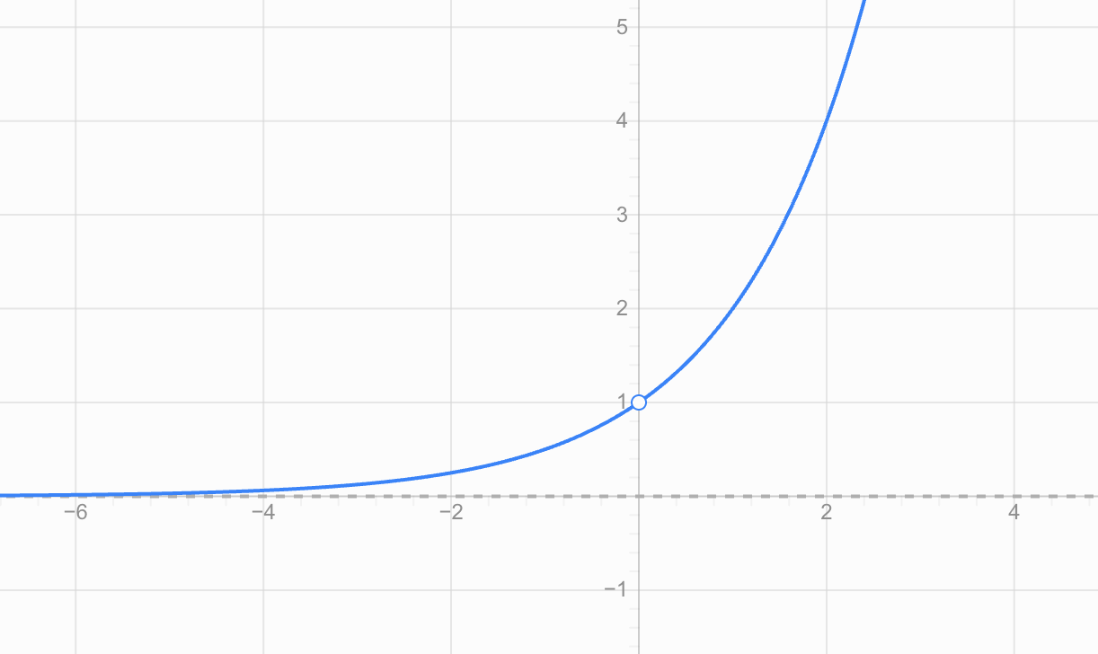
The graph has a distinctive curved shape. As x increases, the value of y increases more and more rapidly.
A few values help explain why:
| x | y = 2ˣ |
|---|---|
| -3 | 1/8 |
| -2 | 1/4 |
| -1 | 1/2 |
| 0 | 1 |
| 1 | 2 |
| 2 | 4 |
| 3 | 8 |
| 4 | 16 |
Notice that when x increases by 1, the value of y doubles.
This constant multiplication is one of the defining features of exponential functions.
Sketching an Exponential Graph
A useful way to sketch an exponential graph is to create a small table of values.
Consider:
y = 3ˣ
Choose several convenient x-values:
| x | y = 3ˣ |
|---|---|
| -2 | 1/9 |
| -1 | 1/3 |
| 0 | 1 |
| 1 | 3 |
| 2 | 9 |
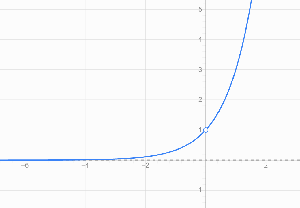
To sketch the graph:
- Choose several x-values on both sides of zero.
- Substitute each x-value into the function.
- Calculate the corresponding y-values.
- Plot the points.
- Connect them with a smooth curve.
- Examine what happens to the curve as x becomes very large or very negative.
Do not connect exponential points with straight line segments. An exponential graph is a smooth curve.
The Importance of x = 0
For a basic exponential function:
y = bˣ
something useful happens when x = 0.
Any non-zero number raised to the power zero equals 1:
b⁰ = 1
Therefore:
y = b⁰ = 1
This means every basic exponential function of the form y = bˣ passes through:
(0, 1)
For example:
- y = 2ˣ passes through (0, 1)
- y = 3ˣ passes through (0, 1)
- y = 5ˣ passes through (0, 1)
- y = (1/2)ˣ passes through (0, 1)
This is a very useful point when sketching.
Exponential Growth
An exponential function shows exponential growth when its values increase as x increases.
For:
y = a(bˣ)
growth occurs when:
b > 1
Examples include:
- y = 2ˣ
- y = 3ˣ
- y = 1.5ˣ
- y = 10ˣ
Compare several growth functions:
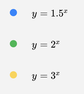
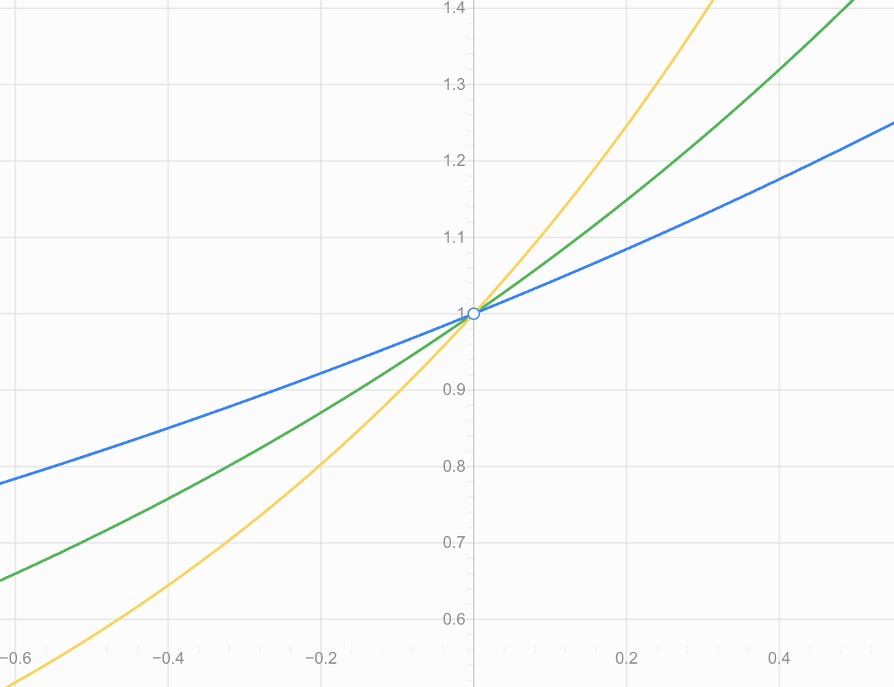
All three increase, but they do not increase at the same rate.
A larger growth factor generally produces faster growth.
For example, beginning at x = 0:
y = 2ˣ
1 → 2 → 4 → 8 → 16
while:
y = 3ˣ
1 → 3 → 9 → 27 → 81
The second function grows much more rapidly.
Growth Means Multiplication
One of the most important ideas about exponential functions is that equal changes in x cause the output to be multiplied by the same factor.
Consider:
y = 5(2ˣ)
| x | y |
|---|---|
| 0 | 5 |
| 1 | 10 |
| 2 | 20 |
| 3 | 40 |
| 4 | 80 |
Each time x increases by 1:
y is multiplied by 2.
This differs from a linear function, where equal changes in x produce equal additions or subtractions.
For example:
Linear: 5, 10, 15, 20, 25 → add 5
Exponential: 5, 10, 20, 40, 80 → multiply by 2
Exponential Decay
Not all exponential functions increase.
An exponential function shows exponential decay when:
0 < b < 1
For example:
y = (1/2)ˣ
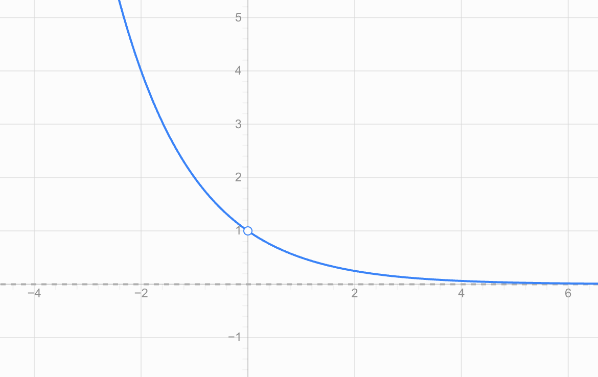
A table of values shows what is happening:
| x | y |
|---|---|
| -2 | 4 |
| -1 | 2 |
| 0 | 1 |
| 1 | 1/2 |
| 2 | 1/4 |
| 3 | 1/8 |
As x increases, y becomes smaller.
However, the values remain positive.
Decay Means Repeated Multiplication Too
Consider:
y = 100(0.5ˣ)
Starting at x = 0:
100 → 50 → 25 → 12.5 → 6.25
Each time x increases by 1, the previous value is multiplied by:
0.5
So exponential decay is not repeated subtraction.
The amount being lost becomes smaller each time because a constant proportion is being removed.
This is why exponential decay curves become flatter as they approach the x-axis.
Growth and Decay Compared
Compare:
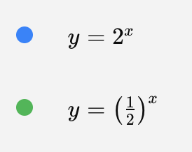
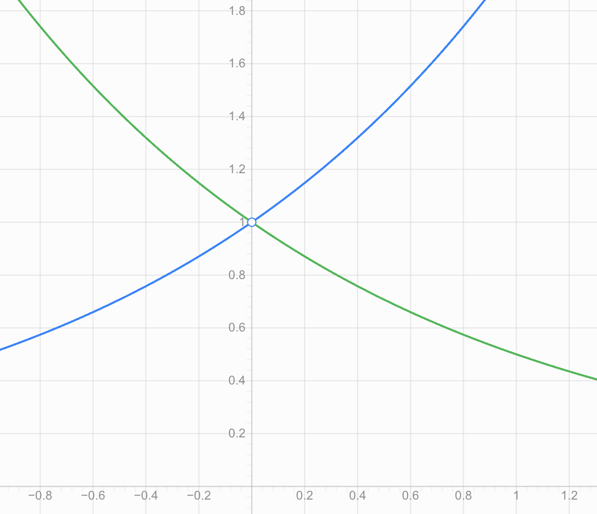
Both graphs:
- pass through (0, 1)
- remain above the x-axis
- have domain consisting of all real numbers
- have range y > 0
- approach y = 0
- never actually reach y = 0
But their directions are different.
Exponential growth: rises from left to right.
Exponential decay: falls from left to right.
Domain of an Exponential Function
The domain is the set of possible x-values.
For a basic exponential function such as:
y = 2ˣ
x can be:
- positive
- negative
- zero
- a fraction
- a decimal
For example:
2⁻³, 2⁰, 2¹·⁵ and 2⁴ are all defined.
Therefore, the domain is:
all real numbers
or:
−∞ < x < ∞
In interval notation:
(−∞, ∞)
This is true for basic exponential functions and their usual transformations.
Range of a Basic Exponential Function
The range is the set of possible y-values.
Consider again:
y = 2ˣ
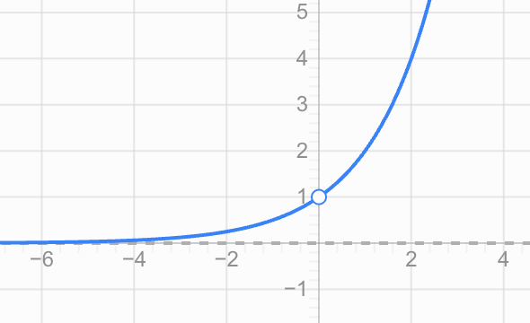
The output is always positive.
It can become extremely small:
0.1
0.01
0.001
and so on.
But it never becomes exactly zero.
It also never becomes negative.
Therefore, for y = 2ˣ:
Range: y > 0
or in interval notation:
(0, ∞)
Horizontal Asymptotes
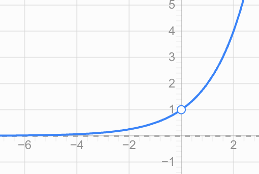
Look carefully at what happens to:
y = 2ˣ
as x becomes increasingly negative.
For example:
2⁻¹ = 0.5
2⁻² = 0.25
2⁻³ = 0.125
2⁻⁴ = 0.0625
2⁻⁵ = 0.03125
The values get closer and closer to zero.
However, 2ˣ never actually equals zero.
The line:
y = 0
is therefore a horizontal asymptote.
A horizontal asymptote is a horizontal line that a graph approaches as x moves far in one direction.
For a basic exponential function:
y = a(bˣ)
the horizontal asymptote is usually:
y = 0
Does an Exponential Graph Touch Its Asymptote?
For a basic positive exponential function, no.
For example:
y = 3ˣ
can become extremely close to zero, but:
3ˣ > 0
for every real value of x.
Therefore, its graph never reaches the x-axis.
This is why the x-axis acts as the horizontal asymptote.
An asymptote describes the long-term behaviour of the graph.
Shifting an Exponential Graph Vertically
Now consider:
y = 2ˣ + 3
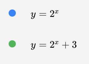
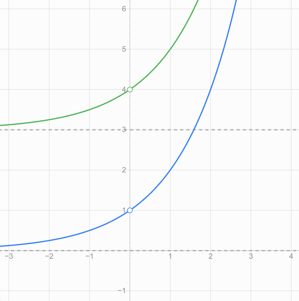
Adding 3 moves the entire graph 3 units upward.
The original function:
y = 2ˣ
has horizontal asymptote:
y = 0
The transformed function:
y = 2ˣ + 3
has horizontal asymptote:
y = 3
Its range also changes.
Instead of:
y > 0
the range becomes:
y > 3
A Useful General Form
A transformed exponential function can be written as:
y = a(bˣ) + k
The value k moves the graph vertically.
Its horizontal asymptote becomes:
y = k
For example:
y = 4(2ˣ) + 5
has horizontal asymptote:
y = 5
and, because the graph is above the asymptote:
Range: y > 5
A Reflection of an Exponential Graph
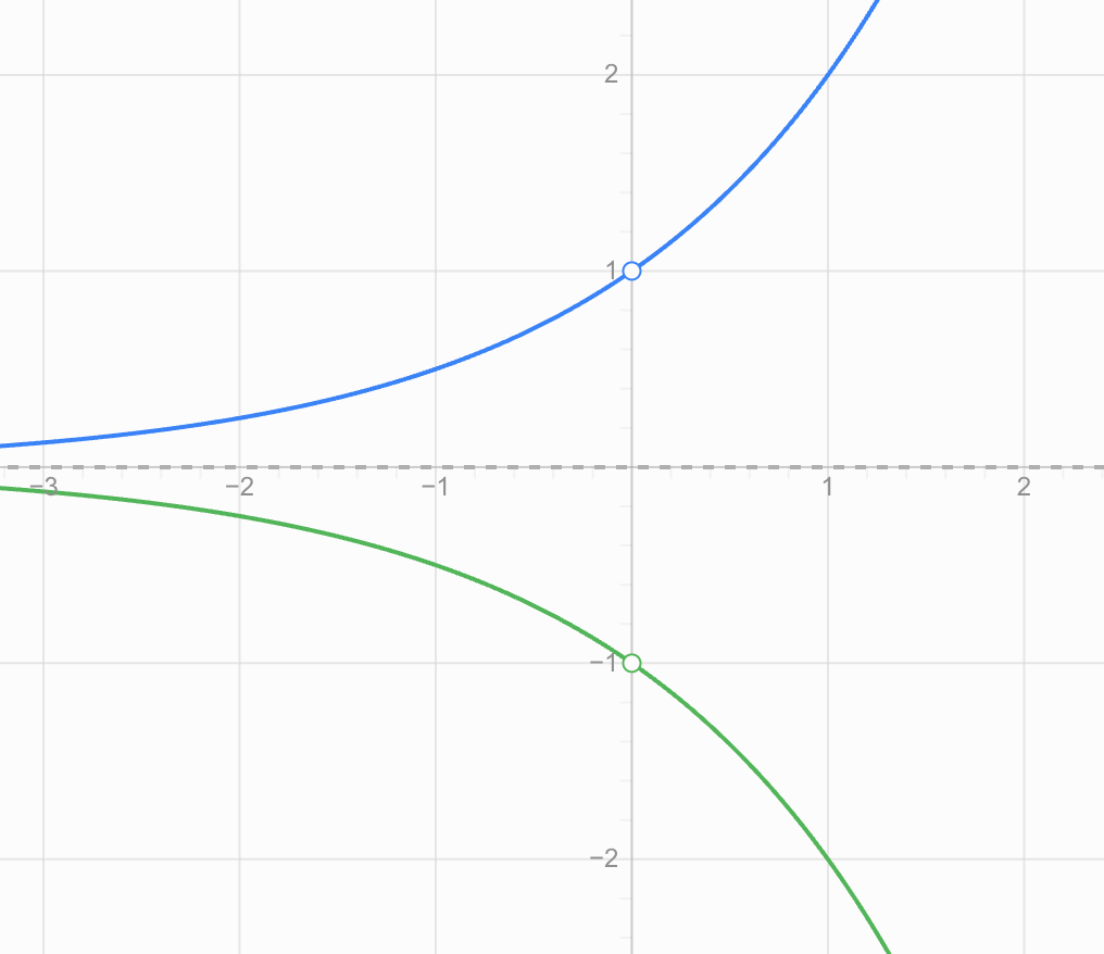
A negative coefficient can reflect an exponential graph across the x-axis.
Compare:
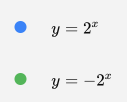
y = 2ˣ
and:
y = −2ˣ
For y = −2ˣ:
- all outputs are negative
- the horizontal asymptote is still y = 0
- the domain is all real numbers
- the range is y < 0
This reminds us that the range is not always y > 0. We must examine the complete function.
Worked Example 1: Sketching an Exponential Growth Function
Sketch:
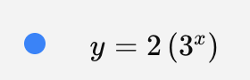
y = 2(3ˣ)
Step 1: Identify the base
The base is:
b = 3
Since:
3 > 1
the function represents exponential growth.
Step 2: Find some points
| x | y = 2(3ˣ) |
|---|---|
| -2 | 2/9 |
| -1 | 2/3 |
| 0 | 2 |
| 1 | 6 |
| 2 | 18 |
Step 3: Identify the asymptote
There is no vertical shift, so:
Horizontal asymptote: y = 0
Step 4: State the domain and range
Domain: all real numbers
Range: y > 0
Step 5: Sketch the curve
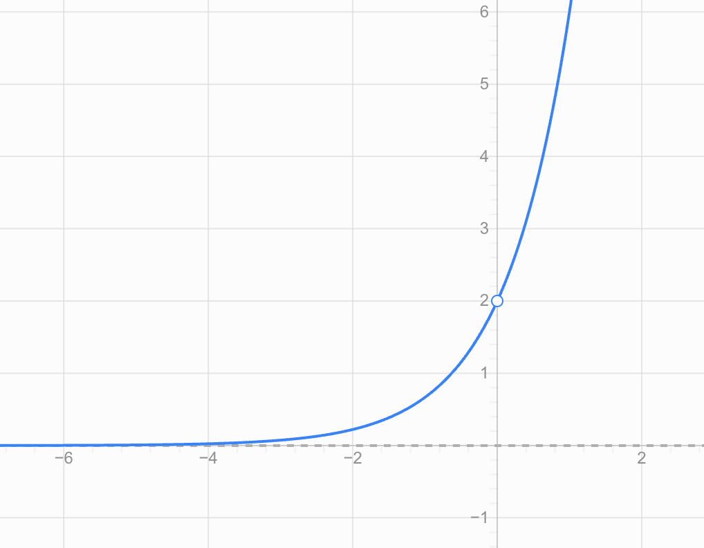
The graph rises increasingly rapidly from left to right.
Worked Example 2: Exponential Decay
Consider:
y = 8(0.5ˣ)
Because:
0 < 0.5 < 1
the function represents exponential decay.
Calculate some values:
| x | y |
|---|---|
| 0 | 8 |
| 1 | 4 |
| 2 | 2 |
| 3 | 1 |
| 4 | 0.5 |
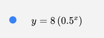
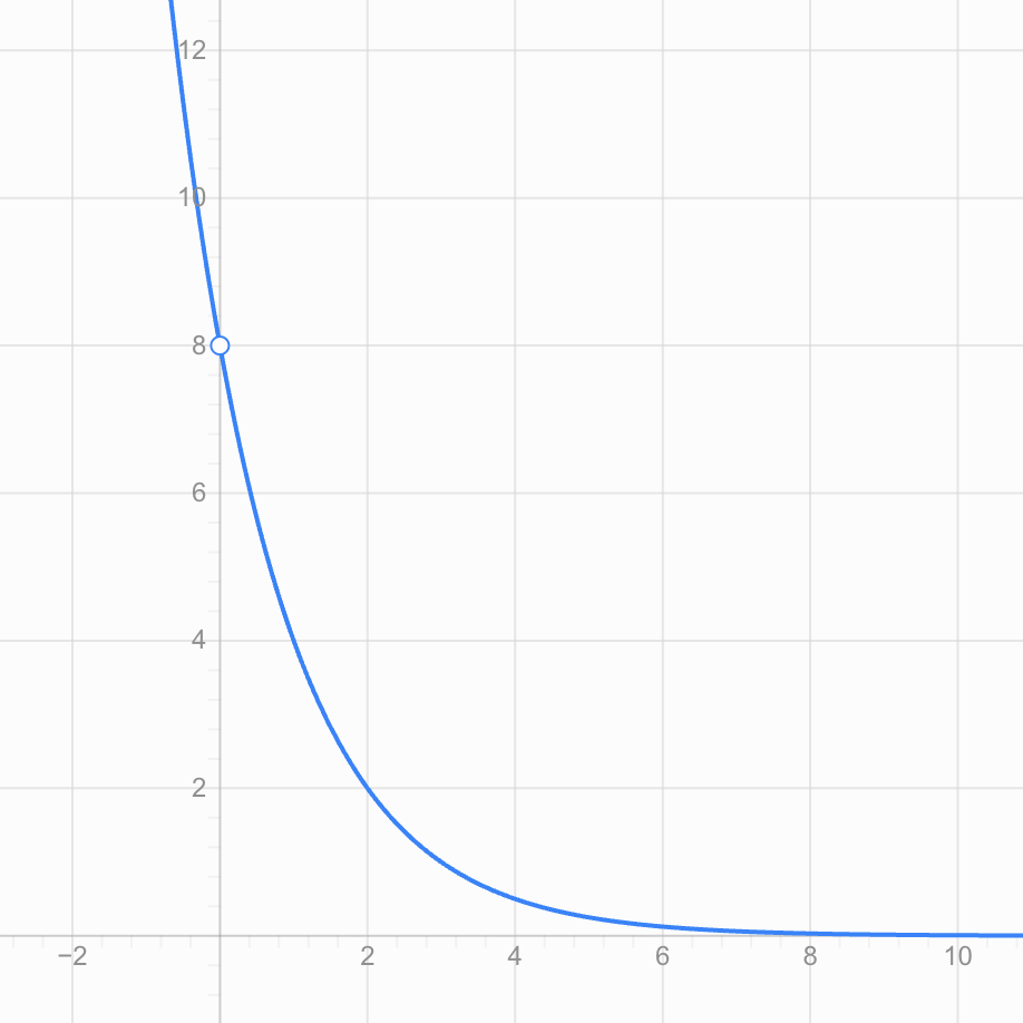
From the graph:
Domain: all real numbers
Range: y > 0
Horizontal asymptote: y = 0
Behaviour: y decreases toward zero as x increases.
Worked Example 3: Finding a Shifted Asymptote
Consider:
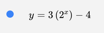
y = 3(2ˣ) − 4
The −4 shifts the basic exponential graph downward by 4 units.
Therefore:
Horizontal asymptote: y = −4
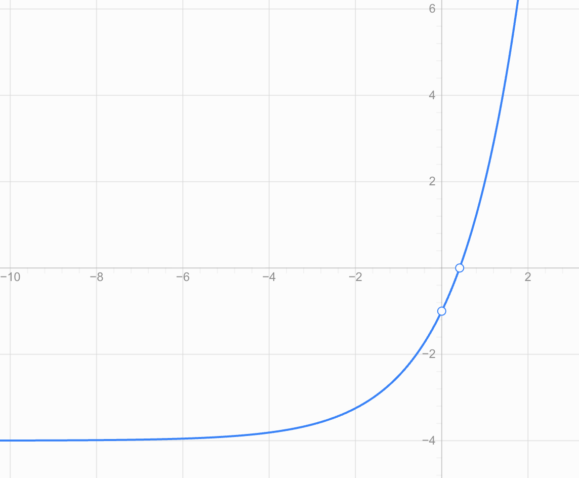
Because 3(2ˣ) is always positive, the graph remains above −4.
Therefore:
Domain: all real numbers
Range: y > −4
Interpreting Exponential Graphs in Context
Exponential functions are useful because many real-world quantities change by a constant percentage or constant multiplication factor.
Examples include:
- population growth
- bacterial growth
- compound interest
- radioactive decay
- depreciation
- cooling models
- spread of information
- some biological growth processes
The graph can tell us much more than whether a quantity is increasing or decreasing.
Example: Bacterial Growth
Suppose a bacterial population is modelled by:
P = 200(2ᵗ)
where:
- P is the bacterial population
- t is time in hours
At t = 0:
P = 200(2⁰)
P = 200
So the initial population is 200 bacteria.
After 1 hour:
P = 200(2¹) = 400
After 2 hours:
P = 200(2²) = 800
After 3 hours:
P = 200(2³) = 1600
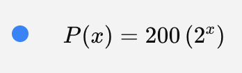
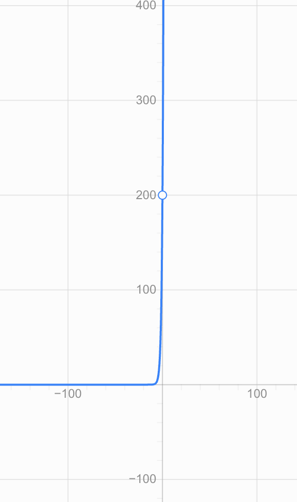
The graph becomes increasingly steep because the population doubles during every equal time interval.
In the real-world context, we would normally restrict the domain to:
t ≥ 0
because negative time may not make sense for the situation being modelled.
Example: Depreciation
Suppose a piece of equipment is initially worth $10,000 and retains 80% of its value each year.
Its value could be modelled by:
V = 10,000(0.8ᵗ)
Because:
0 < 0.8 < 1
this represents exponential decay.
After 1 year:
V = 10,000(0.8)
V = $8,000
After 2 years:
V = 10,000(0.8²)
V = $6,400
After 3 years:
V = 10,000(0.8³)
V = $5,120
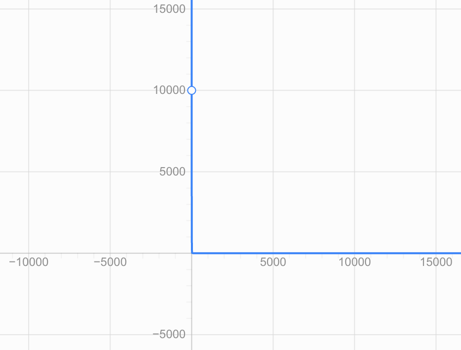
The graph approaches zero but does not reach zero according to the mathematical model.
In reality, an object might eventually have a minimum resale or scrap value, so mathematical models do not always describe reality perfectly forever.
Reading an Exponential Graph
When interpreting an exponential graph, ask several questions.
1. What does the horizontal axis represent?
It might represent:
- time
- distance
- number of periods
- age
2. What does the vertical axis represent?
It might represent:
- population
- money
- mass
- concentration
- temperature difference
3. What is the initial value?
Often this is the value when:
x = 0
4. Is the quantity growing or decaying?
Look at whether the graph rises or falls from left to right.
5. What value does the graph approach?
This can often be identified from the horizontal asymptote.
6. What restrictions make sense?
A mathematical function might allow all real x-values, but the real-world situation may not.
Linear Growth vs Exponential Growth
These two types of growth are easily confused.
Consider:
Linear: y = 2x + 1
Exponential: y = 2ˣ
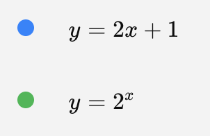
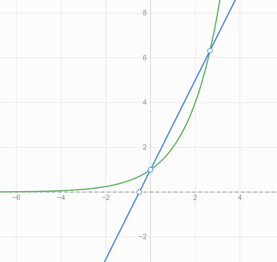
A linear function changes by a constant amount.
An exponential function changes by a constant factor or percentage.
For example:
| x | Linear: 2x + 1 | Exponential: 2ˣ |
|---|---|---|
| 0 | 1 | 1 |
| 1 | 3 | 2 |
| 2 | 5 | 4 |
| 3 | 7 | 8 |
| 4 | 9 | 16 |
| 5 | 11 | 32 |
The exponential function eventually grows much faster.
Common Mistakes
Mistake 1: Thinking exponential growth means constant addition
The sequence:
2, 4, 6, 8, 10
is not exponential.
It increases by 2 each time, so it shows a linear pattern.
The sequence:
2, 4, 8, 16, 32
is exponential because each term is multiplied by 2.
Mistake 2: Thinking an exponential graph eventually reaches its asymptote
For:
y = 2ˣ
the graph approaches y = 0 but never reaches it.
The x-axis is a horizontal asymptote.
Mistake 3: Assuming all exponential graphs increase
Functions with:
b > 1
show exponential growth.
Functions with:
0 < b < 1
show exponential decay.
Mistake 4: Saying the range is always y > 0
That is true for basic positive exponential functions such as:
y = 2ˣ
But transformations can change the range.
For:
y = 2ˣ + 5
the range is:
y > 5
Mistake 5: Confusing x² with 2ˣ
These functions are fundamentally different.
x² → quadratic
2ˣ → exponential
The position of the variable matters.
Key Terms
Exponential function — A function in which the variable occurs in the exponent.
Base — The number being raised to a power.
Exponential growth — An exponential pattern in which values increase by a constant multiplication factor.
Exponential decay — An exponential pattern in which values decrease by a constant multiplication factor between 0 and 1.
Domain — The set of possible input values.
Range — The set of possible output values.
Horizontal asymptote — A horizontal line that a graph approaches as x moves far in one direction.
Initial value — The output at the beginning of a model, commonly when x = 0.
Growth factor — The factor greater than 1 by which a quantity is repeatedly multiplied.
Decay factor — A factor between 0 and 1 by which a quantity is repeatedly multiplied.
Check Your Understanding
-
Is y = 4ˣ an exponential growth or decay function?
-
Is y = (0.3)ˣ growth or decay?
-
What point must the graph of y = 7ˣ pass through?
-
State the domain of y = 5ˣ.
-
State the range of y = 5ˣ.
-
What is the horizontal asymptote of y = 5ˣ?
-
What is the horizontal asymptote of y = 5ˣ + 4?
-
State the range of y = 5ˣ + 4.
-
Create a table of values for y = 2ˣ using x = −2, −1, 0, 1, 2 and sketch the graph.
-
A population is modelled by P = 500(1.2ᵗ). Is the population growing or decaying? Explain how you know.
-
A machine's value is modelled by V = 20,000(0.9ᵗ). What does 20,000 represent? What does 0.9 tell you about the machine's value?
-
Explain why an exponential decay graph can approach zero indefinitely without actually reaching zero.
Key Takeaways
- An exponential function has the variable in the exponent.
- A basic exponential function can be written as y = a(bˣ).
- If b > 1, the function shows exponential growth.
- If 0 < b < 1, the function shows exponential decay.
- Basic exponential functions have a domain of all real numbers.
- A basic positive exponential function has the range y > 0.
- The basic exponential graph has the horizontal asymptote y = 0.
- In y = a(bˣ) + k, the horizontal asymptote is y = k.
- Exponential change involves repeated multiplication, not repeated addition.
- Graphs should always be interpreted using the meaning of their axes and the context of the situation.
Did You Know?
Exponential growth can become surprisingly large very quickly. If a quantity doubles repeatedly, after only 10 doublings it is 1,024 times its original size. After 20 doublings, it is more than one million times its original size. This rapid change is one reason exponential models are so important in areas such as finance, biology, computing, and population studies.
3. Transformations of Exponential Functions
Learning outcomes
- I can apply translations to exponential graphs.
- I can apply reflections and stretches.
- I can determine equations from transformed graphs.
- I can analyse the effects of multiple transformations.
- I can model transformed exponential functions.


4. Exponential Growth and Decay
Learning outcomes
- I can distinguish exponential growth from exponential decay.
- I can model growth and decay using exponential equations.
- I can determine growth and decay rates.
- I can interpret exponential models.
- I can solve practical growth and decay problems.
Exponential Growth and Decay
Many quantities in the real world change by the same percentage over equal periods of time. When this happens, the change can often be modelled using an exponential function.
Examples include:
- populations increasing
- money earning compound interest
- bacteria reproducing
- the value of some products decreasing
- radioactive substances decaying
- medicines being removed from the body
The key idea is that exponential change involves repeated multiplication, rather than repeated addition or subtraction.


Linear Change vs. Exponential Change
It is important to distinguish linear change from exponential change.
A linear relationship changes by the same amount during each interval.
For example:
100, 120, 140, 160, 180
The amount increases by 20 each time.
An exponential relationship changes by the same factor or percentage during each interval.
For example:
100, 120, 144, 172.8, 207.36
Each value is multiplied by:
1.20
This represents a 20% increase each time.
Compare
| Type | What stays constant? | Example |
|---|---|---|
| Linear | Amount added or subtracted | +20 each year |
| Exponential | Percentage or multiplication factor | ×1.20 each year |
This distinction is one of the most important ideas in exponential modelling.
Exponential Growth
Exponential growth occurs when a quantity increases by the same percentage over equal time intervals.
A common model is:
A = A₀(1 + r)ᵗ
where:
- A = amount after time t
- A₀ = initial amount
- r = growth rate written as a decimal
- t = number of time periods
The expression:
1 + r
is called the growth factor.
Example
A population begins at 2,000 and grows by 6% each year.
Initial amount:
A₀ = 2000
Growth rate:
r = 0.06
Growth factor:
1 + 0.06 = 1.06
Therefore:
A = 2000(1.06)ᵗ
This equation models the population after t years.
Converting Percentages to Decimals
Growth and decay rates must normally be written as decimals when substituted into exponential equations.
For example:
5% = 0.05
12% = 0.12
25% = 0.25
0.5% = 0.005
To convert a percentage to a decimal, divide by 100.
For example:
8% ÷ 100 = 0.08
Growth Factors
The growth factor tells us what number the quantity is multiplied by during each time interval.
For growth:
growth factor = 1 + r
Examples
| Growth rate | Growth factor |
|---|---|
| 3% | 1.03 |
| 8% | 1.08 |
| 15% | 1.15 |
| 25% | 1.25 |
| 60% | 1.60 |
If a quantity increases by 12% each year, it retains its original 100% and gains another 12%.
100% + 12% = 112%
112% = 1.12
So it is multiplied by 1.12 each year.
Worked Example: Population Growth
A town has a population of 15,000. Its population grows by 4% each year. Estimate the population after 6 years.
Use:
A = A₀(1 + r)ᵗ
Substitute:
A = 15000(1.04)⁶
A ≈ 18,980
So the predicted population after 6 years is approximately:
18,980 people
Notice that we do not simply calculate 4% of 15,000 and add that same amount six times. Each year's growth is based on the new population.


Exponential Decay
Exponential decay occurs when a quantity decreases by the same percentage over equal time intervals.
A common model is:
A = A₀(1 − r)ᵗ
The expression:
1 − r
is called the decay factor.
Example
A machine is worth $20,000 and loses 15% of its value each year.
Initial value:
A₀ = 20000
Decay rate:
r = 0.15
Decay factor:
1 − 0.15 = 0.85
Therefore:
A = 20000(0.85)ᵗ
Each year, the machine retains 85% of its previous value.
Decay Factors
For exponential decay:
decay factor = 1 − r
Examples
| Decay rate | Decay factor |
|---|---|
| 5% | 0.95 |
| 10% | 0.90 |
| 18% | 0.82 |
| 25% | 0.75 |
| 40% | 0.60 |
A factor between 0 and 1 indicates exponential decay.
For example:
A = 500(0.72)ᵗ
Since:
0 < 0.72 < 1
the model represents decay.
The decay rate is:
1 − 0.72 = 0.28
Therefore:
decay rate = 28%
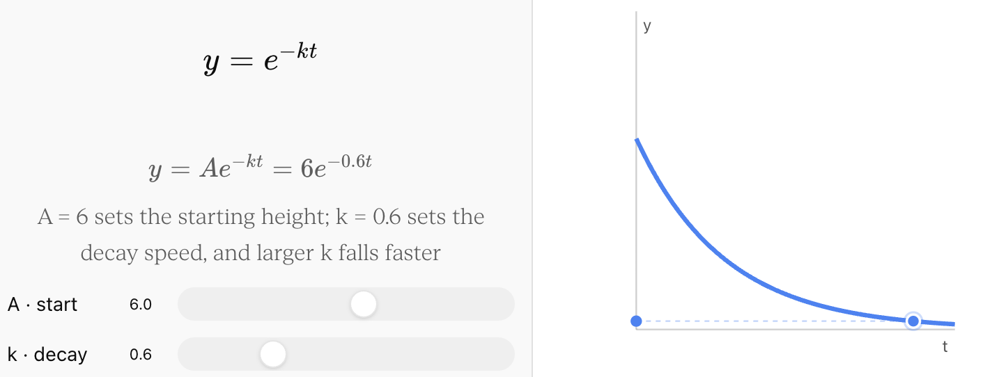
The decreasing behaviour of an exponential model can be explored directly here:


5. Applications of Exponential Functions
Learning outcomes
- I can model compound interest.
- I can model population growth.
- I can model radioactive decay.
- I can analyse depreciation problems.
- I can solve authentic applications of exponential change.
Applications of Exponential Functions
Exponential functions are useful whenever a quantity changes by the same percentage or multiplication factor over equal intervals of time. They allow us to model situations in finance, biology, physics, economics, technology, and many other fields.
Common applications include:
- compound interest
- population growth
- radioactive decay
- depreciation
- bacterial growth
- medication concentration
- inflation
- spread of information or disease
- cooling and other decay processes
The important skill is not simply substituting numbers into an equation. We need to decide which exponential model fits the situation, interpret its parameters, perform the calculation, and decide whether the answer makes sense.


Recognizing an Exponential Situation
A situation may be exponential if a quantity changes by a constant percentage rather than a constant amount.
For example, suppose an investment increases by 5% each year.
If it begins at $1,000:
Year 0: $1,000
Year 1: $1,050
Year 2: $1,102.50
Year 3: $1,157.63
The amount added each year changes, but the percentage remains 5%.
This is exponential growth.
A general exponential model can be written as:
A = A₀bᵗ
where:
- A = amount after time t
- A₀ = initial amount
- b = growth or decay factor
- t = number of time periods
For growth:
b > 1
For decay:
0 < b < 1
Compound Interest
Compound interest occurs when interest is calculated not only on the original amount invested but also on interest that has already been earned.
This creates exponential growth.
For annual compounding, a basic model is:
A = P(1 + r)ᵗ
where:
- A = final amount
- P = principal or initial investment
- r = annual interest rate as a decimal
- t = number of years
The expression 1 + r is the growth factor.
For example, an interest rate of 6% gives:
r = 0.06
Growth factor:
1 + 0.06 = 1.06
So the investment is multiplied by 1.06 each year.
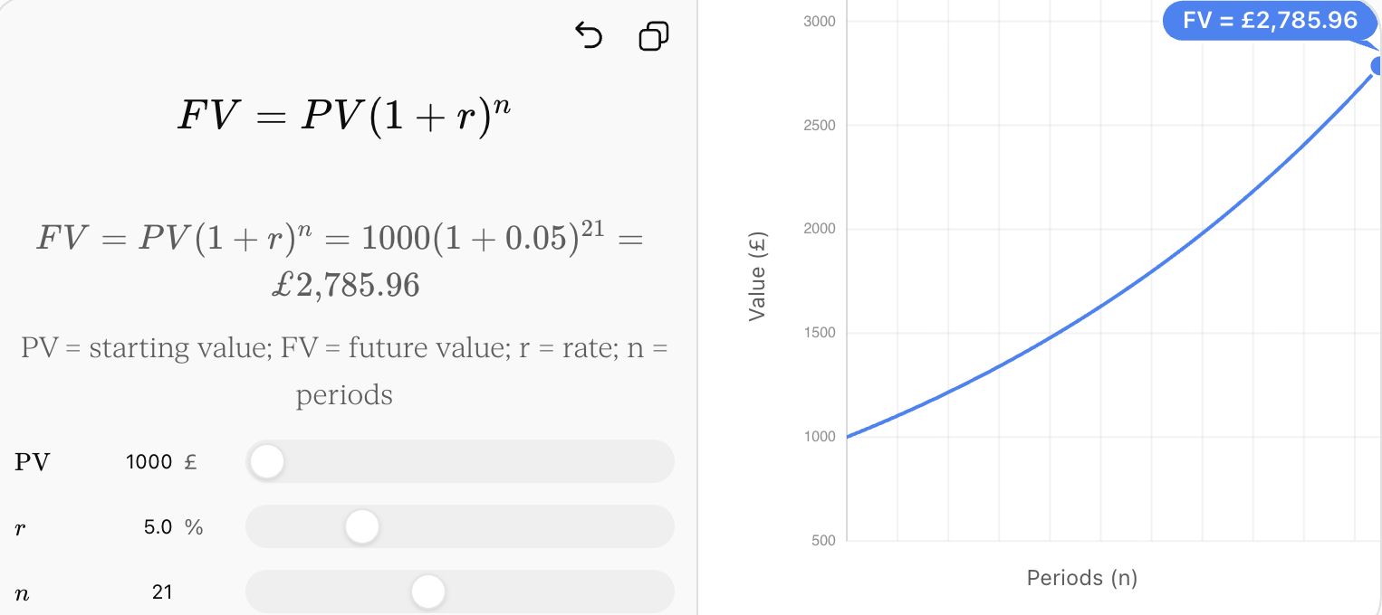
The effect of repeated compounding can be explored here:
Worked Example: Compound Interest
Suppose $5,000 is invested at 4% annual compound interest for 8 years.
Identify the values:
P = 5000
r = 0.04
t = 8
Substitute:
A = 5000(1.04)⁸
A ≈ 6842.85
The investment will be worth approximately:
$6,842.85
The amount of interest earned is:
6842.85 − 5000 = 1842.85
Therefore, approximately $1,842.85 in interest was earned.
Compound Interest More Than Once Per Year
Interest may be compounded several times each year.
A more general formula is:
A = P(1 + r/n)^(nt)
where:
- P = principal
- r = annual interest rate
- n = number of compounding periods per year
- t = number of years
For example:
- annually → n = 1
- semi-annually → n = 2
- quarterly → n = 4
- monthly → n = 12
Example
$2,000 is invested at 6% annual interest compounded monthly for 5 years.
P = 2000
r = 0.06
n = 12
t = 5
A = 2000(1 + 0.06/12)^(12 × 5)
A = 2000(1.005)⁶⁰
A ≈ 2697.70
The account will contain approximately $2,697.70.


Population Growth
Populations can sometimes be modelled using exponential functions when they increase by approximately the same percentage during each time interval.
A simple population model is:
P = P₀(1 + r)ᵗ
where:
- P = future population
- P₀ = initial population
- r = growth rate
- t = time
Worked Example
A town has 25,000 people and grows by 3% each year. Estimate its population after 10 years.
P₀ = 25000
r = 0.03
t = 10
P = 25000(1.03)¹⁰
P ≈ 33,598
The model predicts approximately:
33,598 people
Interpreting a Population Model
Suppose:
P = 4800(1.025)ᵗ
We can interpret the model directly.
4800 represents the initial population.
1.025 is the growth factor.
Therefore:
1.025 − 1 = 0.025
The growth rate is:
2.5% per time period
If t is measured in years, the population increases by 2.5% per year.
When Exponential Population Growth Becomes Unrealistic
Exponential models assume that the same proportional growth can continue.
Real populations eventually encounter limits such as:
- available food
- water
- space
- disease
- competition
- predation
- habitat availability
As a result, exponential growth may be useful over a limited period but unrealistic over very long periods.
In ecology, a logistic model may be more appropriate when growth slows as the population approaches the environment's carrying capacity.
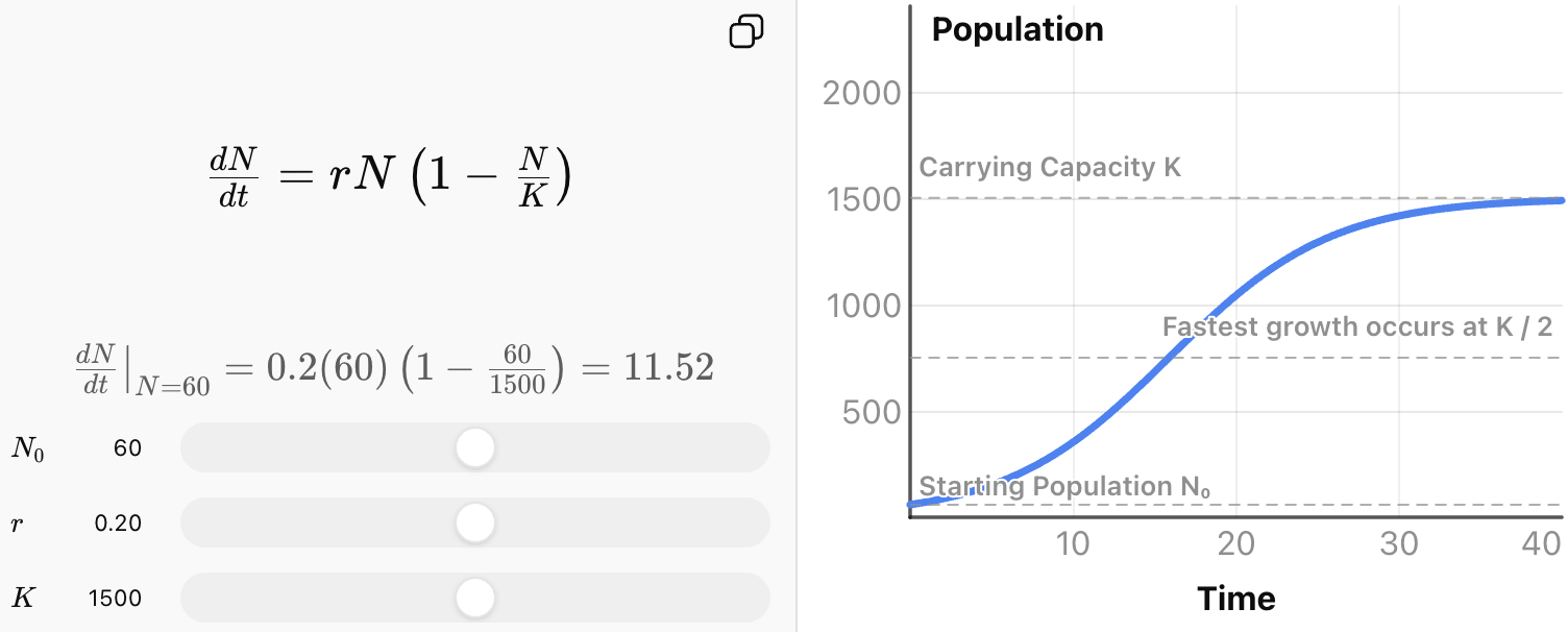
This is an important lesson about mathematical modelling: a mathematically correct calculation is only useful if the model itself is appropriate.


Radioactive Decay
Radioactive substances contain unstable nuclei that decay over time.
Although individual radioactive nuclei decay unpredictably, a large sample follows a predictable exponential pattern.
A decay model can be written as:
N = N₀(1 − r)ᵗ
where:
- N = amount remaining
- N₀ = initial amount
- r = decay rate
- t = time
Radioactive decay is often described using half-life.
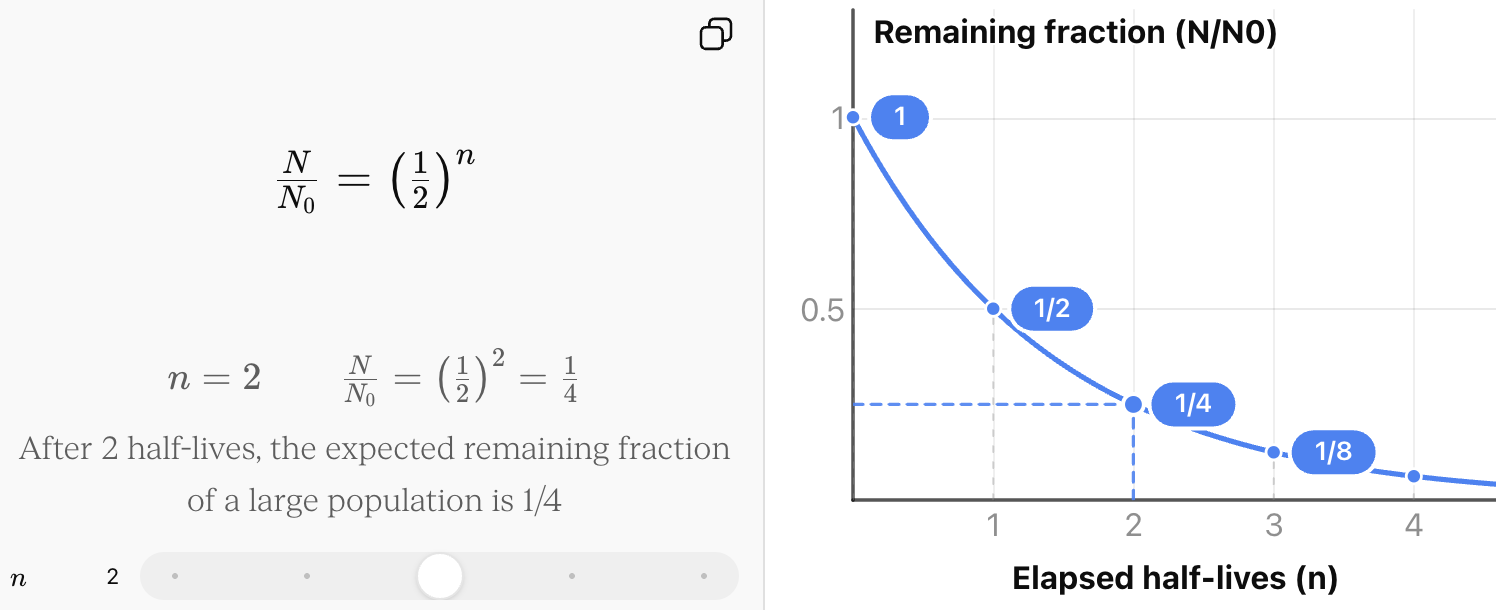
Half-Life
The half-life of a radioactive substance is the time required for half of the radioactive nuclei in a large sample to decay.
A half-life model can be written as:
N = N₀(1/2)^(t/h)
where:
- N = amount remaining
- N₀ = initial amount
- t = elapsed time
- h = half-life
Each complete half-life multiplies the amount by 1/2.
Worked Example: Radioactive Decay
A radioactive isotope has a half-life of 6 years. A sample initially contains 320 mg.
How much remains after 18 years?
First determine the number of half-lives:
18 ÷ 6 = 3 half-lives
Now repeatedly halve the quantity:
320 → 160 → 80 → 40
Therefore:
40 mg remains.
We can also use the equation:
N = 320(1/2)^(18/6)
N = 320(1/2)³
N = 320 × 1/8
N = 40 mg
Radioactive Decay Never Simply Subtracts the Same Amount
Suppose a 400 g sample has a half-life of 5 years.
After 5 years:
400 → 200 g
After another 5 years:
200 → 100 g
After another 5 years:
100 → 50 g
The amount lost is different each time:
- first interval: 200 g lost
- second interval: 100 g lost
- third interval: 50 g lost
But the fraction lost remains constant.
This is why radioactive decay is exponential rather than linear.


Depreciation
Depreciation describes a decrease in the value of an asset over time.
Cars, computers, machinery, phones, and other equipment may lose a percentage of their value each year.
A common exponential depreciation model is:
V = V₀(1 − r)ᵗ
where:
- V = value after time t
- V₀ = original value
- r = depreciation rate
- t = number of time periods
Worked Example: Vehicle Depreciation
A car costs $36,000 and depreciates by 18% each year.
Find its estimated value after 4 years.
Initial value:
V₀ = 36000
Depreciation rate:
r = 0.18
Decay factor:
1 − 0.18 = 0.82
Model:
V = 36000(0.82)ᵗ
After four years:
V = 36000(0.82)⁴
V ≈ 16,874.77
The model predicts a value of approximately:
$16,874.77
Interpreting Depreciation Correctly
An 18% depreciation rate does not mean that the asset loses 18% of its original value every year.
Instead, it loses 18% of its current value.
For the $36,000 car:
First year:
36000 × 0.82 = 29520
Second year:
29520 × 0.82 = 24206.40
The dollar amount lost decreases even though the percentage remains 18%.
This repeated proportional decrease creates exponential decay.


Comparing Common Exponential Applications
| Application | Growth or decay? | Typical model |
|---|---|---|
| Compound interest | Growth | A = P(1 + r)ᵗ |
| Population increase | Growth | P = P₀(1 + r)ᵗ |
| Radioactive decay | Decay | N = N₀(1/2)^(t/h) |
| Percentage depreciation | Decay | V = V₀(1 − r)ᵗ |
Although the contexts are very different, the mathematical structure is similar.
Each model contains:
initial amount × repeated multiplication
Recognizing this common structure makes exponential applications much easier to solve.
Determining the Rate from an Equation
Sometimes the model is already provided.
Consider:
P = 8000(1.06)ᵗ
The growth factor is:
1.06
Therefore:
1.06 − 1 = 0.06
The growth rate is:
6%
Now consider:
V = 24000(0.87)ᵗ
The decay factor is:
0.87
Therefore:
1 − 0.87 = 0.13
The depreciation rate is:
13%
Building a Model from a Description
Suppose a problem states:
A wildlife population begins at 12,500 and decreases by 4% each year.
Identify the initial value:
P₀ = 12500
Convert the rate:
4% = 0.04
Since this is decay:
1 − 0.04 = 0.96
Therefore:
P = 12500(0.96)ᵗ
Once the model has been created, it can be used to predict the population at different times.
Solving an Authentic Application
Suppose a company purchases a piece of equipment for $85,000. The equipment loses 12% of its value each year.
The company plans to sell it after 7 years.
Build the Model
Initial value:
V₀ = 85000
Depreciation rate:
r = 0.12
Decay factor:
1 − 0.12 = 0.88
Therefore:
V = 85000(0.88)ᵗ
Calculate the Value After 7 Years
V = 85000(0.88)⁷
V ≈ 34,738
The model predicts that the equipment will be worth approximately $34,738 after seven years.
Interpret the Result
The model assumes that the equipment continues to lose 12% of its current value every year.
In reality, its resale value could also depend on:
- condition
- maintenance
- technological changes
- market demand
- inflation
This illustrates the difference between a mathematical model and the real system it represents.
A Strategy for Exponential Application Problems
When solving a practical problem, first identify the initial amount, then decide whether the situation involves growth or decay. Convert the percentage to a decimal and determine the multiplication factor.
For growth:
factor = 1 + r
For decay:
factor = 1 − r
Then write the exponential model, substitute the required time, calculate, and interpret the answer using appropriate units.
Finally, ask:
Does the answer make sense in the context of the problem?
Checking Your Answer
Suppose an investment begins at $4,000 and grows by 7%.
If your answer after ten years is $2,500, something is wrong because a growth model should produce a value greater than the initial amount.
Similarly, suppose a car depreciates from $30,000.
If your model predicts that it is worth $45,000 after several years, the result does not match the situation.
Estimating the expected direction of change before calculating is a useful way to catch mistakes.
Limitations of Exponential Models
Exponential models are powerful, but they are simplifications.
A population may not grow at the same rate forever.
An interest rate may change.
A vehicle's depreciation rate may vary as it ages.
Environmental conditions may change.
Radioactive decay is highly predictable for large samples, but the exact decay time of an individual nucleus cannot be predicted.
A good mathematical model should therefore be evaluated by asking:
- What assumptions does the model make?
- Is the rate likely to remain constant?
- Over what time interval is the model reasonable?
- Are important real-world factors missing?
- Is the prediction an interpolation or a long-range extrapolation?
Common Mistakes
Using the percentage instead of the multiplier
For 8% growth:
Incorrect factor: 0.08
Correct factor: 1.08
For 8% decay:
Correct factor: 0.92
Treating exponential change as linear
A 10% annual decrease does not mean subtracting the same amount every year.
The 10% is calculated from the new value each year.
Using growth when the situation describes decay
Words such as depreciates, decreases, decays, loses, falls, and declines usually indicate decay.
Confusing the amount remaining with the amount lost
A decay factor of 0.72 means 72% remains.
Therefore:
100% − 72% = 28% is lost
Using the wrong time units
If a half-life is given in years, the time in the equation must also be expressed in years.
Rounding too early
Keep several decimal places during calculations and round the final answer appropriately.
Key Terms
Exponential model — an equation representing repeated proportional growth or decay.
Compound interest — interest calculated on both the original principal and previously accumulated interest.
Principal — the original amount of money invested or borrowed.
Interest rate — the percentage by which an investment or debt changes over a specified time period.
Compounding period — the interval at which interest is calculated and added.
Population growth — an increase in population that may be modelled exponentially when the proportional growth rate remains approximately constant.
Radioactive decay — the spontaneous transformation of unstable atomic nuclei, producing an exponential decrease in the number of undecayed nuclei in a large sample.
Half-life — the time required for half of the radioactive nuclei in a large sample to decay.
Depreciation — the decrease in the monetary value of an asset over time.
Growth factor — the multiplier 1 + r used for exponential growth.
Decay factor — the multiplier 1 − r used for exponential decay.
Initial value — the value of the quantity when t = 0.
Mathematical model — a mathematical representation used to describe or predict a real-world situation.
Extrapolation — using a model to predict values beyond the range of observed data.
Key Takeaways
- Exponential functions model situations involving repeated percentage change.
- Compound interest is an important application of exponential growth.
- Population growth can often be approximated exponentially over limited periods.
- Radioactive decay follows an exponential pattern and is commonly described using half-life.
- Percentage depreciation can be modelled using exponential decay.
- Growth uses a factor of 1 + r.
- Decay uses a factor of 1 − r.
- The initial value is the amount when t = 0.
- The time units in the model must match the time units of the rate.
- Exponential models can make useful predictions, but their assumptions should always be considered.
- A complete solution should include the model, calculation, units, and interpretation.
Check Your Understanding
- $6,000 is invested at 5% annual compound interest. Write an exponential model for the investment.
- Use your model to determine the value of the $6,000 investment after 8 years.
- A population of 18,000 grows by 2.5% each year. Write an exponential model.
- Estimate the population after 12 years.
- A radioactive sample begins with 640 mg and has a half-life of 4 years. How much remains after 12 years?
- A car originally costs $42,000 and depreciates by 16% each year. Write an exponential model for its value.
- Estimate the value of the car after 5 years.
- Explain why a depreciation factor of 0.91 represents a 9% decrease, not a 91% decrease.
- An investment is modelled by A = 8500(1.045)ᵗ. Identify the initial investment and annual growth rate.
- A machine's value is modelled by V = 56000(0.88)ᵗ. Identify its initial value and annual depreciation rate.
- A bacteria population doubles every 3 hours and begins with 400 bacteria. Write an exponential model and determine the population after 15 hours.
- A city currently has 150,000 people and has been growing by 4% annually. Explain why using this model to predict the city's population 200 years into the future might produce an unrealistic result.