Random Variables

Introduction

Probability helps us describe events that involve uncertainty. However, in many situations, we want to go beyond determining whether an event will occur. We also want to calculate and analyse the numerical results of random experiments.

For example:

• How many heads will appear when three coins are tossed?

• How many customers will enter a shop during an hour?

• How long will a student wait for a bus?

• What is the expected score when rolling a fair die?

• How much money might a business earn from a game of chance?

These situations can be studied using random variables.

A random variable assigns a numerical value to each possible outcome of a random experiment.

Random variables are fundamental to probability distributions, expected values, statistics, economics, insurance, scientific research, and decision-making.

What Is a Random Variable?

A random variable is a function that assigns a numerical value to each outcome of a random experiment.

Random variables are usually represented by capital letters such as:

X, Y, or Z

A particular value of a random variable is usually represented by a lowercase letter such as x.

Example: Rolling a Die

Suppose a fair six-sided die is rolled.

Let X represent the number shown.

The possible values are:

X = 1, 2, 3, 4, 5, or 6

Each value has a probability of 1/6.

Example: Tossing Coins

Suppose two fair coins are tossed.

Let X represent the number of heads.

The possible outcomes are:

HH, HT, TH, TT

The possible values of X are:

X = 0, 1, or 2

Notice that different outcomes can produce the same value of a random variable.

Both HT and TH produce X = 1.

Important Distinction

An outcome describes what happened during the experiment.

A random variable assigns a number to that outcome.

Types of Random Variables

Random variables are commonly classified into two main types:

• Discrete random variables.

• Continuous random variables.

The distinction depends on the possible numerical values the variable can take.

Discrete Random Variables

A discrete random variable takes values from a finite or countably infinite set.

Discrete random variables often involve counting.

Examples include:

• Number of students absent from class.

• Number of goals scored in a football match.

• Number of defective products in a shipment.

• Number of heads in five coin tosses.

• Number of customers arriving during an hour.

Example: Number of Defective Products

Suppose a factory inspects four products.

Let X represent the number of defective products.

Possible values:

X = 0, 1, 2, 3, or 4

X cannot equal 1.5 because we are counting whole products.

Important Characteristics

Discrete random variables:

• Have distinct possible values.

• Can be represented using probability tables.

• Often use bar graphs.

• May have a finite or countably infinite number of possible values.

Continuous Random Variables

A continuous random variable can take any real value within an interval, at least in the mathematical model.

Continuous random variables often involve measurements.

Examples include:

• Height.

• Mass.

• Temperature.

• Time.

• Distance.

• Speed.

• Rainfall amount.

Example: Waiting Time

Suppose X represents the time, in minutes, a passenger waits for a bus.

Possible values might include:

2 minutes

2.5 minutes

2.75 minutes

2.751 minutes

and many other values.

The variable is continuous because waiting time can take any value within the modelled interval.

Important Characteristics

Continuous random variables:

• Are often based on measurements.

• Can take infinitely many possible values within an interval.

• Are commonly represented using probability density curves.

• Have probabilities associated with intervals rather than individual exact values.

Comparing Discrete and Continuous Random Variables

Important Observation

The type of random variable depends on what is being measured or counted.

For example:

• Number of cars passing a checkpoint is discrete.

• Time between cars is continuous.

• Number of raindrops is discrete.

• Amount of rainfall is continuous.

Probability Distributions

A probability distribution describes the possible values of a random variable and their associated probabilities.

For a discrete random variable, a probability distribution can be represented using a table.

Example: Rolling a Fair Die

Let X represent the number shown on a fair six-sided die.

Requirements of a Valid Discrete Probability Distribution

Every probability must satisfy:

0 ≤ P(X = x) ≤ 1

The probabilities must add to 1:

ΣP(X = x) = 1

These conditions ensure that the distribution represents a valid probability model.

Checking a Probability Distribution

Consider the following table:

Step 1: Check Individual Probabilities

Every probability lies between 0 and 1.

Step 2: Add the Probabilities

0.10 + 0.25 + 0.40 + 0.25

= 1.00

Conclusion

This is a valid probability distribution.

Invalid Example

Suppose the probabilities were:

0.20, 0.35, 0.40, 0.25

Their sum would be:

0.20 + 0.35 + 0.40 + 0.25 = 1.20

Because the probabilities add to more than 1, the distribution is invalid.

Constructing a Probability Distribution

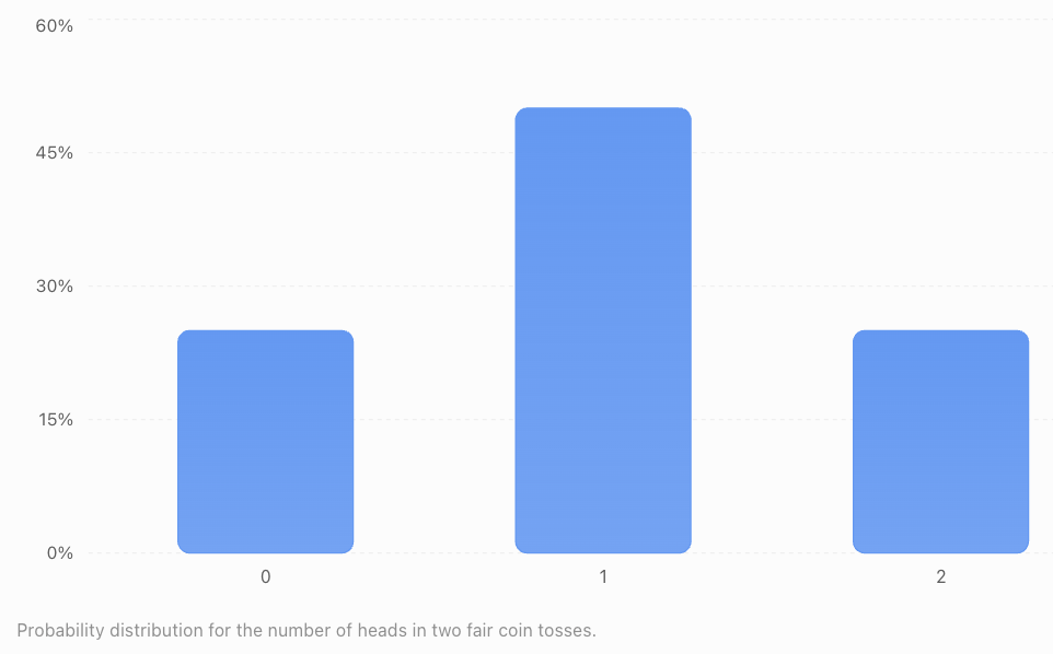
Suppose two fair coins are tossed.

Let X represent the number of heads.

Step 1: List the Outcomes

HH, HT, TH, TT

Each outcome has probability 1/4.

Step 2: Count the Heads

Step 3: Calculate the Probabilities

P(X = 0) = 1/4

P(X = 1) = 2/4 = 1/2

P(X = 2) = 1/4

Step 4: Create the Distribution

Step 5: Interpret

The most likely result is exactly one head.

There is a 50% probability of obtaining one head.

There is a 25% probability of obtaining no heads and a 25% probability of obtaining two heads.

Reading Probability Notation

Probability statements use mathematical notation.

P(X = 2)

This means:

The probability that X equals 2.

P(X < 3)

This means:

The probability that X is less than 3.

P(X ≤ 3)

This means:

The probability that X is less than or equal to 3.

P(X ≥ 2)

This means:

The probability that X is greater than or equal to 2.

Example

Consider:

Find P(X ≥ 2).

Solution

P(X ≥ 2) = P(X = 2) + P(X = 3)

= 0.40 + 0.30

P(X ≥ 2) = 0.70

Therefore, there is a 70% probability that X is at least 2.

Cumulative Probabilities

A cumulative probability gives the probability that a random variable is less than or equal to a specified value.

The cumulative distribution function is:

F(x) = P(X ≤ x)

Worked Example

Consider:

Interpretation

P(X ≤ 1) = 0.30

P(X ≤ 2) = 0.70

P(X ≤ 3) = 1.00

The cumulative probabilities increase or remain constant as x increases.

They eventually reach 1 for a finite distribution.

Expected Value

The expected value of a random variable is its probability-weighted average.

It represents the long-run average outcome of an experiment repeated many times under the same conditions.

Expected value is often represented by:

E(X)

For a discrete random variable:

E(X) = Σ[x × P(X = x)]

This means:

Multiply each possible value by its probability, then add the results.

Important Observation

The expected value does not have to be one of the possible outcomes.

For example, the expected number of heads in three fair coin tosses is 1.5.

A single experiment cannot produce exactly 1.5 heads, but the average across many repetitions can approach 1.5.

Calculating Expected Value: Fair Die

Let X represent the result of rolling a fair six-sided die.

Step 1: Create the Probability Table

Step 2: Add the Weighted Values

E(X) = (1 + 2 + 3 + 4 + 5 + 6)/6

E(X) = 21/6

E(X) = 3.5

Interpretation

The expected result of rolling a fair die is 3.5.

A single roll cannot produce 3.5.

However, the average result over many rolls tends toward 3.5.

Calculating Expected Value: Unequal Probabilities

Consider the probability distribution:

Find E(X).

Step 1: Multiply Each Value by Its Probability

0 × 0.10 = 0

1 × 0.20 = 0.20

2 × 0.40 = 0.80

3 × 0.30 = 0.90

Step 2: Add

E(X) = 0 + 0.20 + 0.80 + 0.90

E(X) = 1.90

Interpretation

The long-run average value of X is 1.9.

This does not mean that 1.9 is an actual possible outcome.

Expected Value and Games of Chance

Expected value is useful when analysing games, prizes, and financial decisions.

Worked Example: A Prize Game

A game costs $3 to play.

A player rolls a fair six-sided die.

• Rolling a 6 wins a $12 prize.

• Rolling any other number wins nothing.

Let X represent the player's net gain.

Step 1: Identify the Possible Net Gains

If the player rolls a 6:

Net gain = $12 − $3 = $9

Otherwise:

Net gain = $0 − $3 = −$3

Step 2: Create the Distribution

Step 3: Calculate Expected Value

E(X) = 9(1/6) + (−3)(5/6)

E(X) = 9/6 − 15/6

E(X) = −6/6

E(X) = −$1

Interpretation

The expected net gain is negative $1 per game.

Over many repetitions, the player would lose an average of approximately $1 per game.

Important Distinction

Expected value describes a long-run average.

It does not predict the exact result of an individual game.

Fair and Unfair Games

A game is often described as fair when the expected net gain is zero for each participant.

Fair Game

E(X) = 0

The player neither gains nor loses money on average.

Unfavourable Game

E(X) < 0

The player loses money on average.

Favourable Game

E(X) > 0

The player gains money on average.

Example

Suppose a game costs $2.

A player has a 1/4 probability of winning $8 and a 3/4 probability of winning nothing.

Expected prize:

E(prize) = 8(1/4) + 0(3/4)

E(prize) = $2

Expected net gain:

$2 − $2 = $0

The game is fair in terms of expected monetary value.

Expected Value in Business

Businesses often use expected value when making decisions involving uncertainty.

Example: Product Sales

A small shop estimates the number of products it may sell during a day.

Calculate Expected Sales

E(X) = 0(0.10) + 1(0.20) + 2(0.30) + 3(0.25) + 4(0.15)

E(X) = 0 + 0.20 + 0.60 + 0.75 + 0.60

E(X) = 2.15 products

Interpretation

The expected number of products sold per day is 2.15.

The shop cannot sell 0.15 of a whole product in an ordinary transaction.

However, its long-run daily average may approach 2.15 products.

Expected Value of a Binomial Random Variable

Some random variables count the number of successes in repeated independent trials.

For example:

• Number of heads in ten coin tosses.

• Number of successful shots in five attempts.

• Number of defective products in a sample.

If X follows a binomial distribution with n trials and success probability p:

E(X) = np

Worked Example

A basketball player has a 70% probability of making a free throw.

Assume each attempt is independent and the probability remains constant.

The player takes 20 free throws.

Find the expected number of successful shots.

Step 1: Identify the Values

n = 20

p = 0.70

Step 2: Calculate

E(X) = 20 × 0.70

E(X) = 14

Interpretation

The expected number of successful shots is 14.

The player may actually make more or fewer than 14 shots in a particular set of attempts.

Continuous Probability Distributions

Continuous random variables are described using probability density functions.

A probability density function is often represented by:

f(x)

The total area under the density curve is 1.

Probabilities are represented by areas under the curve.

Important Properties

For a continuous random variable:

P(a ≤ X ≤ b)

represents the area under the density curve between a and b.

The probability of an exact individual value is zero:

P(X = a) = 0

This does not mean the value is impossible.

It means a single point has zero width and therefore zero area under a continuous probability density curve.

Example: Uniform Continuous Distribution

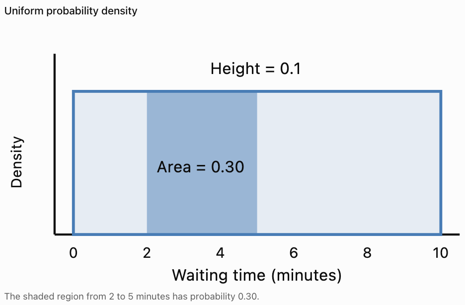
Suppose a bus arrives at a random time during a 10-minute interval.

Assume every arrival time within the interval is equally likely.

Let X represent the waiting time, in minutes.

X is uniformly distributed between 0 and 10.

Probability Density

The density is constant:

f(x) = 1/10, for 0 ≤ x ≤ 10

The total area is:

10 × 1/10 = 1

Worked Example

Find the probability that the waiting time is between 2 and 5 minutes.

Step 1: Identify the Interval Width

5 − 2 = 3 minutes

Step 2: Calculate the Area

P(2 ≤ X ≤ 5) = 3 × 1/10

P(2 ≤ X ≤ 5) = 0.30

Interpretation

There is a 30% probability that the waiting time lies between 2 and 5 minutes.

Expected Value of a Continuous Random Variable

The expected value of a continuous random variable is calculated using integration.

E(X) = ∫ x f(x) dx

The integral is taken over the possible values of X.

This is the continuous equivalent of multiplying each discrete value by its probability and adding.

Uniform Distribution Example

For a continuous uniform distribution between a and b:

E(X) = (a + b)/2

If a waiting time is uniformly distributed between 0 and 10 minutes:

E(X) = (0 + 10)/2

E(X) = 5 minutes

Interpretation

The expected waiting time is five minutes.

An individual passenger may wait more or less than five minutes.

Probability Distributions and Graphs

Different random variables are represented using different types of graphs.

Discrete Probability Distribution

A discrete probability distribution is commonly represented using separate bars.

The height of each bar represents the probability of an individual value.

Continuous Probability Distribution

A continuous probability distribution is represented using a density curve.

The area under the curve over an interval represents probability.

Important Distinction

For discrete variables, probabilities can be associated with individual values.

For continuous variables, probabilities are associated with intervals.

Variance and Standard Deviation of Random Variables

Expected value describes the centre of a probability distribution.

However, two random variables can have the same expected value and different levels of variability.

Variance and standard deviation measure how spread out the possible values are around the expected value.

Variance of a Discrete Random Variable

Var(X) = Σ[(x − μ)²P(X = x)]

where:

μ = E(X)

An equivalent formula is:

Var(X) = E(X²) − [E(X)]²

Standard Deviation

σ = √Var(X)

Worked Example

Consider:

We previously found:

E(X) = 1

Calculate E(X²):

E(X²) = 0²(0.25) + 1²(0.50) + 2²(0.25)

E(X²) = 0 + 0.50 + 1

E(X²) = 1.5

Therefore:

Var(X) = 1.5 − 1²

Var(X) = 0.5

Standard deviation:

σ = √0.5

σ ≈ 0.707

Interpretation

The expected value is 1.

The standard deviation is approximately 0.707.

This describes the spread of the possible outcomes around the expected value.

Transforming Random Variables

Sometimes a random variable is multiplied by a constant or increased by a fixed amount.

Suppose:

Y = aX + b

where a and b are constants.

The expected value follows:

E(Y) = aE(X) + b

Worked Example

A worker earns $15 for each item completed, plus a fixed daily payment of $20.

Let X represent the number of items completed.

Suppose:

E(X) = 8

The worker's daily earnings are:

Y = 15X + 20

Calculate the expected earnings:

E(Y) = 15E(X) + 20

E(Y) = 15(8) + 20

E(Y) = $140

Important Observation

Expected value can be used to predict average earnings, costs, or other quantities when they are calculated from a random variable.

Real-World Application: Insurance

Insurance companies use probability models to estimate expected claims.

Example

Suppose an insurance company estimates that a particular type of claim has:

• A 2% probability of occurring during a year.

• An average payment of $5,000 if it occurs.

In this simplified model, assume the payment is exactly $5,000 when a claim occurs.

Let X represent the claim payment.

Expected claim payment:

E(X) = 0(0.98) + 5,000(0.02)

E(X) = $100

Interpretation

The expected claim payment is $100 per policy per year.

Actual insurance premiums may be higher because they also account for administration, uncertainty, capital requirements, and other costs.

Real-World Application: Scientific Experiments

Scientists often use random variables to represent uncertain experimental outcomes.

Examples include:

• Number of radioactive decays during a time interval.

• Number of particles detected.

• Measurement errors.

• Time between events.

• Number of successful trials.

Example

A detector records the number of particles arriving during one minute.

Let X represent the number of detected particles.

X is discrete because it counts individual particles.

If instead we measure the time between detections, that waiting time can be modelled as continuous.

This demonstrates how closely related scientific measurements can involve different types of random variables.

Real-World Application: Weather

Weather predictions frequently involve probability distributions.

For example:

• Amount of rainfall.

• Daily maximum temperature.

• Wind speed.

• Number of thunderstorms.

• Time until the next rainfall event.

Example

Let X represent the number of thunderstorms occurring during a day.

X is discrete.

Let Y represent the amount of rainfall in millimetres.

Y is continuous in a measurement model, although recorded values may be rounded.

Interpretation

Random variables allow meteorologists to describe uncertainty rather than predict only a single value.

Probability distributions can provide information about both typical conditions and the likelihood of unusual events.

Common Mistakes

Confusing an outcome with a random variable

An outcome describes what happens. A random variable assigns a numerical value to that outcome.

Assuming every random variable is continuous

Counts are usually discrete.

Assuming every random variable is discrete

Measurements are often modelled as continuous.

Forgetting that probabilities must add to 1

A discrete probability distribution must have total probability 1.

Using probabilities greater than 1

Probabilities must lie between 0 and 1.

Forgetting to multiply values by their probabilities

Expected value is a weighted average, not necessarily the ordinary average of the possible values.

Assuming expected value must be a possible outcome

Expected values can be fractional even when the random variable counts whole objects.

Confusing expected prize with expected net gain

Net gain must account for the cost of participating.

Assuming expected value predicts an individual result

Expected value describes a long-run average.

Confusing probability density with probability

For continuous distributions, probability is represented by area under the density curve.

Assuming an exact continuous value has positive probability

Under a continuous probability model, the probability of any single exact value is zero.

Ignoring the conditions of a probability model

Assumptions such as independence, constant probabilities, and fairness must be appropriate.

Key Terms

• Random Experiment: Process with uncertain outcomes.

• Outcome: Possible result of a random experiment.

• Sample Space: Set of all possible outcomes.

• Random Variable: Function assigning numerical values to outcomes.

• Discrete Random Variable: Random variable with finite or countably infinite possible values.

• Continuous Random Variable: Random variable taking values across continuous intervals.

• Probability Distribution: Description of possible values and their probabilities.

• Probability Mass Function: Function giving probabilities of individual discrete values.

• Probability Density Function: Function whose area over an interval gives continuous probability.

• Cumulative Distribution Function: Function giving P(X ≤ x).

• Expected Value: Probability-weighted average of a random variable.

• Mean of a Random Variable: Another name for its expected value.

• Variance: Measure of the spread of a probability distribution.

• Standard Deviation: Square root of variance.

• Probability: Numerical measure of the likelihood of an event.

• Independent Events: Events whose occurrence does not affect each other's probabilities.

• Fair Game: Game with an expected net gain of zero.

• Net Gain: Winnings minus costs.

• Long-Run Average: Average approached over many repetitions under stable conditions.

• Binomial Distribution: Distribution describing successes in a fixed number of independent trials with constant success probability.

• Uniform Distribution: Distribution with equal probabilities for discrete values or constant density across a continuous interval.

• Probability Model: Mathematical representation of uncertainty.

• Weighted Average: Average accounting for the relative importance or probability of each value.

• Cumulative Probability: Probability that a variable is at or below a specified value.

Key Takeaways

• A random variable assigns numerical values to outcomes of a random experiment.

• Random variables may be discrete or continuous.

• Discrete random variables often involve counting.

• Continuous random variables often involve measurement.

• A probability distribution describes possible values and their probabilities.

• All probabilities in a discrete distribution must be between 0 and 1.

• The probabilities of all possible discrete values must add to 1.

• Expected value is a probability-weighted average.

• For a discrete variable, E(X) = Σ[x × P(X = x)].

• Expected value does not need to be a possible individual outcome.

• Expected value is useful for analysing games, business decisions, insurance, and scientific experiments.

• A fair game has an expected net gain of zero.

• For continuous variables, probabilities correspond to areas under density curves.

• The total area under a probability density curve is 1.

• Variance and standard deviation describe the spread of a random variable.

• Random variables provide mathematical tools for making decisions under uncertainty.

Check Your Understanding

Random Variables

1. Define a random variable.

2. Explain the difference between a discrete and continuous random variable.

3. Is the number of students absent from school discrete or continuous?

4. Is the height of a student discrete or continuous?

5. Is the time required to complete an examination discrete or continuous?

Probability Distributions

6. State the two requirements of a valid discrete probability distribution.

7. Determine whether probabilities 0.20, 0.30, 0.40, and 0.10 form a valid distribution.

8. Determine whether probabilities 0.25, 0.35, 0.50, and 0.20 form a valid distribution.

9. A random variable has P(X = 0) = 0.2, P(X = 1) = 0.5, and P(X = 2) = 0.3. Find P(X ≥ 1).

10. For the same distribution, find P(X ≤ 1).

Expected Value

11. Calculate the expected value of a fair six-sided die.

12. Calculate E(X) for X = 0, 1, 2 with probabilities 0.2, 0.5, 0.3.

13. Explain why expected value does not have to be a possible outcome.

14. A game costs $2. A player has a 1/4 chance of winning $8 and otherwise wins nothing. Find the expected net gain.

15. A basketball player has an 80% chance of making each free throw. Find the expected number of successful shots in 15 independent attempts.

Continuous Random Variables

16. What does the area under a probability density curve represent?

17. What is the total area under a valid probability density curve?

18. Why is P(X = 5) = 0 for a continuous random variable?

19. A waiting time is uniformly distributed between 0 and 20 minutes. Find the probability of waiting between 5 and 10 minutes.

20. Find the expected waiting time for the same uniform distribution.

Answer Key

Extended Challenge

Classifying Random Variables

1. Classify the number of books borrowed from a library during a day.

2. Classify the mass of a randomly selected apple.

3. Classify the number of customers arriving at a shop.

4. Classify the temperature of a classroom.

5. Explain why the number of rainfall events and the amount of rainfall are different types of random variables.

Constructing Distributions

6. Construct the probability distribution for the number of heads in three fair coin tosses.

7. Verify that the probabilities add to 1.

8. Calculate the expected number of heads.

9. Find the probability of obtaining at least two heads.

10. Find the probability of obtaining fewer than two heads.

Expected Value Applications

11. A game awards $10 with probability 0.2 and nothing otherwise. Calculate the expected prize.

12. If the game costs $3, calculate the expected net gain.

13. A company sells 0, 1, 2, or 3 products with probabilities 0.1, 0.2, 0.4, and 0.3. Find the expected number sold.

14. Each product earns $25 in profit. Find the expected daily profit.

15. Explain why a business might prefer a decision with lower expected profit but less uncertainty.

Continuous Distributions

16. A waiting time is uniformly distributed between 0 and 30 minutes. Find P(10 ≤ X ≤ 20).

17. Find the expected waiting time.

18. Explain why the probability of waiting exactly 15 minutes is zero in the continuous model.

19. Explain how a probability density function differs from a discrete probability mass function.

20. Describe a real-world situation in which a continuous probability distribution would be useful.

Final Investigation: Designing a Probability Game

You are designing a game using a fair six-sided die.

The game costs $4 to play.

Players receive prizes according to the following rules:

• Rolling a 1 or 2 wins nothing.

• Rolling a 3 or 4 wins $3.

• Rolling a 5 wins $6.

• Rolling a 6 wins $12.

Complete the investigation.

1. Define a random variable X representing the prize awarded.

2. List all possible values of X.

3. Calculate the probability of each prize.

4. Construct a probability distribution table.

5. Verify that the probabilities add to 1.

6. Construct a bar graph of the distribution.

7. Calculate the expected prize.

8. Calculate the expected net gain after paying the $4 entry fee.

9. Determine whether the game is fair.

10. Explain whether the game favours the player or the organiser.

11. Calculate the probability of winning any prize.

12. Calculate the probability of winning more than the entry fee.

13. Calculate the probability of losing money.

14. Calculate the probability of breaking even.

15. Determine the expected total net gain for a player over 100 games.

16. Explain why the actual results of 100 games may differ from the expected result.

17. Determine an entry fee that would make the game fair.

18. Suggest a change to one prize that would make the game fair while keeping the $4 entry fee.

19. Explain how probability distributions can help people evaluate games of chance.

20. Write a conclusion describing the role of expected value in financial decision-making.