Probability Distributions
| Site: | Young Education |
| Course: | Statistics |
| Book: | Probability Distributions |
| Printed by: | Guest user |
| Date: | Monday, 9 November 2026, 4:38 PM |
1. Random Variables
Learning outcomes
- I can define random variables.
- I can distinguish between discrete and continuous random variables.
- I can calculate expected values.
- I can interpret probability distributions.
- I can solve problems involving random variables.
Random Variables
Introduction
Probability helps us describe events that involve uncertainty. However, in many situations, we want to go beyond determining whether an event will occur. We also want to calculate and analyse the numerical results of random experiments.
For example:
-
How many heads will appear when three coins are tossed?
-
How many customers will enter a shop during an hour?
-
How long will a student wait for a bus?
-
What is the expected score when rolling a fair die?
-
How much money might a business earn from a game of chance?
These situations can be studied using random variables.
A random variable assigns a numerical value to each possible outcome of a random experiment.
Random variables are fundamental to probability distributions, expected values, statistics, economics, insurance, scientific research, and decision-making.


What Is a Random Variable?
A random variable is a function that assigns a numerical value to each outcome of a random experiment.
Random variables are usually represented by capital letters such as:
X, Y, or Z
A particular value of a random variable is usually represented by a lowercase letter such as x.
Example: Rolling a Die
Suppose a fair six-sided die is rolled.
Let X represent the number shown.
The possible values are:
X = 1, 2, 3, 4, 5, or 6
Each value has a probability of 1/6.
Example: Tossing Coins
Suppose two fair coins are tossed.
Let X represent the number of heads.
The possible outcomes are:
HH, HT, TH, TT
|
Outcome |
Number of heads (X) |
|---|---|
|
HH |
2 |
|
HT |
1 |
|
TH |
1 |
|
TT |
0 |
The possible values of X are:
X = 0, 1, or 2
Notice that different outcomes can produce the same value of a random variable.
Both HT and TH produce X = 1.
Important Distinction
An outcome describes what happened during the experiment.
A random variable assigns a number to that outcome.
Types of Random Variables
Random variables are commonly classified into two main types:
-
Discrete random variables.
-
Continuous random variables.
The distinction depends on the possible numerical values the variable can take.
Discrete Random Variables
A discrete random variable takes values from a finite or countably infinite set.
Discrete random variables often involve counting.
Examples include:
-
Number of students absent from class.
-
Number of goals scored in a football match.
-
Number of defective products in a shipment.
-
Number of heads in five coin tosses.
-
Number of customers arriving during an hour.
Example: Number of Defective Products
Suppose a factory inspects four products.
Let X represent the number of defective products.
Possible values:
X = 0, 1, 2, 3, or 4
X cannot equal 1.5 because we are counting whole products.
Important Characteristics
Discrete random variables:
-
Have distinct possible values.
-
Can be represented using probability tables.
-
Often use bar graphs.
-
May have a finite or countably infinite number of possible values.

Continuous Random Variables
A continuous random variable can take any real value within an interval, at least in the mathematical model.
Continuous random variables often involve measurements.
Examples include:
-
Height.
-
Mass.
-
Temperature.
-
Time.
-
Distance.
-
Speed.
-
Rainfall amount.
Example: Waiting Time
Suppose X represents the time, in minutes, a passenger waits for a bus.
Possible values might include:
2 minutes
2.5 minutes
2.75 minutes
2.751 minutes
and many other values.
The variable is continuous because waiting time can take any value within the modelled interval.
Important Characteristics
Continuous random variables:
-
Are often based on measurements.
-
Can take infinitely many possible values within an interval.
-
Are commonly represented using probability density curves.
-
Have probabilities associated with intervals rather than individual exact values.

Comparing Discrete and Continuous Random Variables
|
Feature |
Discrete |
Continuous |
|---|---|---|
|
Possible values |
Finite or countably infinite |
Values across continuous intervals |
|
Common application |
Counting |
Measuring |
|
Example |
Number of children |
Height of children |
|
Graph |
Probability bars |
Probability density curve |
|
Individual value probability |
May be positive |
Zero in a continuous model |
|
Probability calculation |
Add probabilities |
Find area under a density curve |
Important Observation
The type of random variable depends on what is being measured or counted.
For example:
-
Number of cars passing a checkpoint is discrete.
-
Time between cars is continuous.
-
Number of raindrops is discrete.
-
Amount of rainfall is continuous.
Probability Distributions
A probability distribution describes the possible values of a random variable and their associated probabilities.
For a discrete random variable, a probability distribution can be represented using a table.
Example: Rolling a Fair Die
Let X represent the number shown on a fair six-sided die.
|
X |
P(X = x) |
|---|---|
|
1 |
1/6 |
|
2 |
1/6 |
|
3 |
1/6 |
|
4 |
1/6 |
|
5 |
1/6 |
|
6 |
1/6 |
Requirements of a Valid Discrete Probability Distribution
Every probability must satisfy:
0 ≤ P(X = x) ≤ 1
The probabilities must add to 1:
ΣP(X = x) = 1
These conditions ensure that the distribution represents a valid probability model.
Checking a Probability Distribution
Consider the following table:
|
X |
Probability |
|---|---|
|
0 |
0.10 |
|
1 |
0.25 |
|
2 |
0.40 |
|
3 |
0.25 |
Step 1: Check Individual Probabilities
Every probability lies between 0 and 1.
Step 2: Add the Probabilities
0.10 + 0.25 + 0.40 + 0.25
= 1.00
Conclusion
This is a valid probability distribution.
Invalid Example
Suppose the probabilities were:
0.20, 0.35, 0.40, 0.25
Their sum would be:
0.20 + 0.35 + 0.40 + 0.25 = 1.20
Because the probabilities add to more than 1, the distribution is invalid.
Constructing a Probability Distribution
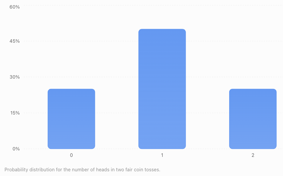
Suppose two fair coins are tossed.
Let X represent the number of heads.
Step 1: List the Outcomes
HH, HT, TH, TT
Each outcome has probability 1/4.
Step 2: Count the Heads
|
Outcome |
X |
|---|---|
|
TT |
0 |
|
HT |
1 |
|
TH |
1 |
|
HH |
2 |
Step 3: Calculate the Probabilities
P(X = 0) = 1/4
P(X = 1) = 2/4 = 1/2
P(X = 2) = 1/4
Step 4: Create the Distribution
|
Number of heads (X) |
Probability |
|---|---|
|
0 |
0.25 |
|
1 |
0.50 |
|
2 |
0.25 |
|
Total |
1.00 |
Step 5: Interpret
The most likely result is exactly one head.
There is a 50% probability of obtaining one head.
There is a 25% probability of obtaining no heads and a 25% probability of obtaining two heads.
Reading Probability Notation
Probability statements use mathematical notation.
P(X = 2)
This means:
The probability that X equals 2.
P(X < 3)
This means:
The probability that X is less than 3.
P(X ≤ 3)
This means:
The probability that X is less than or equal to 3.
P(X ≥ 2)
This means:
The probability that X is greater than or equal to 2.
Example
Consider:
|
X |
Probability |
|---|---|
|
0 |
0.10 |
|
1 |
0.20 |
|
2 |
0.40 |
|
3 |
0.30 |
Find P(X ≥ 2).
Solution
P(X ≥ 2) = P(X = 2) + P(X = 3)
= 0.40 + 0.30
P(X ≥ 2) = 0.70
Therefore, there is a 70% probability that X is at least 2.
Cumulative Probabilities
A cumulative probability gives the probability that a random variable is less than or equal to a specified value.
The cumulative distribution function is:
F(x) = P(X ≤ x)
Worked Example
Consider:
|
X |
Probability |
Cumulative probability |
|---|---|---|
|
0 |
0.10 |
0.10 |
|
1 |
0.20 |
0.30 |
|
2 |
0.40 |
0.70 |
|
3 |
0.30 |
1.00 |
Interpretation
P(X ≤ 1) = 0.30
P(X ≤ 2) = 0.70
P(X ≤ 3) = 1.00
The cumulative probabilities increase or remain constant as x increases.
They eventually reach 1 for a finite distribution.
Expected Value
The expected value of a random variable is its probability-weighted average.
It represents the long-run average outcome of an experiment repeated many times under the same conditions.
Expected value is often represented by:
E(X)
For a discrete random variable:
E(X) = Σ[x × P(X = x)]
This means:
Multiply each possible value by its probability, then add the results.
Important Observation
The expected value does not have to be one of the possible outcomes.
For example, the expected number of heads in three fair coin tosses is 1.5.
A single experiment cannot produce exactly 1.5 heads, but the average across many repetitions can approach 1.5.
Calculating Expected Value: Fair Die
Let X represent the result of rolling a fair six-sided die.
Step 1: Create the Probability Table
|
X |
P(X = x) |
x × P(X = x) |
|---|---|---|
|
1 |
1/6 |
1/6 |
|
2 |
1/6 |
2/6 |
|
3 |
1/6 |
3/6 |
|
4 |
1/6 |
4/6 |
|
5 |
1/6 |
5/6 |
|
6 |
1/6 |
6/6 |
Step 2: Add the Weighted Values
E(X) = (1 + 2 + 3 + 4 + 5 + 6)/6
E(X) = 21/6
E(X) = 3.5
Interpretation
The expected result of rolling a fair die is 3.5.
A single roll cannot produce 3.5.
However, the average result over many rolls tends toward 3.5.

Calculating Expected Value: Unequal Probabilities
Consider the probability distribution:
|
X |
Probability |
|---|---|
|
0 |
0.10 |
|
1 |
0.20 |
|
2 |
0.40 |
|
3 |
0.30 |
Find E(X).
Step 1: Multiply Each Value by Its Probability
0 × 0.10 = 0
1 × 0.20 = 0.20
2 × 0.40 = 0.80
3 × 0.30 = 0.90
Step 2: Add
E(X) = 0 + 0.20 + 0.80 + 0.90
E(X) = 1.90
Interpretation
The long-run average value of X is 1.9.
This does not mean that 1.9 is an actual possible outcome.
Expected Value and Games of Chance
Expected value is useful when analysing games, prizes, and financial decisions.
Worked Example: A Prize Game
A game costs $3 to play.
A player rolls a fair six-sided die.
-
Rolling a 6 wins a $12 prize.
-
Rolling any other number wins nothing.
Let X represent the player's net gain.
Step 1: Identify the Possible Net Gains
If the player rolls a 6:
Net gain = $12 − $3 = $9
Otherwise:
Net gain = $0 − $3 = −$3
Step 2: Create the Distribution
|
Net gain (X) |
Probability |
|---|---|
|
$9 |
1/6 |
|
−$3 |
5/6 |
Step 3: Calculate Expected Value
E(X) = 9(1/6) + (−3)(5/6)
E(X) = 9/6 − 15/6
E(X) = −6/6
E(X) = −$1
Interpretation
The expected net gain is negative $1 per game.
Over many repetitions, the player would lose an average of approximately $1 per game.
Important Distinction
Expected value describes a long-run average.
It does not predict the exact result of an individual game.
Fair and Unfair Games
A game is often described as fair when the expected net gain is zero for each participant.
Fair Game
E(X) = 0
The player neither gains nor loses money on average.
Unfavourable Game
E(X) < 0
The player loses money on average.
Favourable Game
E(X) > 0
The player gains money on average.
Example
Suppose a game costs $2.
A player has a 1/4 probability of winning $8 and a 3/4 probability of winning nothing.
Expected prize:
E(prize) = 8(1/4) + 0(3/4)
E(prize) = $2
Expected net gain:
$2 − $2 = $0
The game is fair in terms of expected monetary value.
Expected Value in Business
Businesses often use expected value when making decisions involving uncertainty.
Example: Product Sales
A small shop estimates the number of products it may sell during a day.
|
Products sold |
Probability |
|---|---|
|
0 |
0.10 |
|
1 |
0.20 |
|
2 |
0.30 |
|
3 |
0.25 |
|
4 |
0.15 |
Calculate Expected Sales
E(X) = 0(0.10) + 1(0.20) + 2(0.30) + 3(0.25) + 4(0.15)
E(X) = 0 + 0.20 + 0.60 + 0.75 + 0.60
E(X) = 2.15 products
Interpretation
The expected number of products sold per day is 2.15.
The shop cannot sell 0.15 of a whole product in an ordinary transaction.
However, its long-run daily average may approach 2.15 products.

Expected Value of a Binomial Random Variable
Some random variables count the number of successes in repeated independent trials.
For example:
-
Number of heads in ten coin tosses.
-
Number of successful shots in five attempts.
-
Number of defective products in a sample.
If X follows a binomial distribution with n trials and success probability p:
E(X) = np
Worked Example
A basketball player has a 70% probability of making a free throw.
Assume each attempt is independent and the probability remains constant.
The player takes 20 free throws.
Find the expected number of successful shots.
Step 1: Identify the Values
n = 20
p = 0.70
Step 2: Calculate
E(X) = 20 × 0.70
E(X) = 14
Interpretation
The expected number of successful shots is 14.
The player may actually make more or fewer than 14 shots in a particular set of attempts.
Continuous Probability Distributions
Continuous random variables are described using probability density functions.
A probability density function is often represented by:
f(x)
The total area under the density curve is 1.
Probabilities are represented by areas under the curve.
Important Properties
For a continuous random variable:
P(a ≤ X ≤ b)
represents the area under the density curve between a and b.
The probability of an exact individual value is zero:
P(X = a) = 0
This does not mean the value is impossible.
It means a single point has zero width and therefore zero area under a continuous probability density curve.
Example: Uniform Continuous Distribution
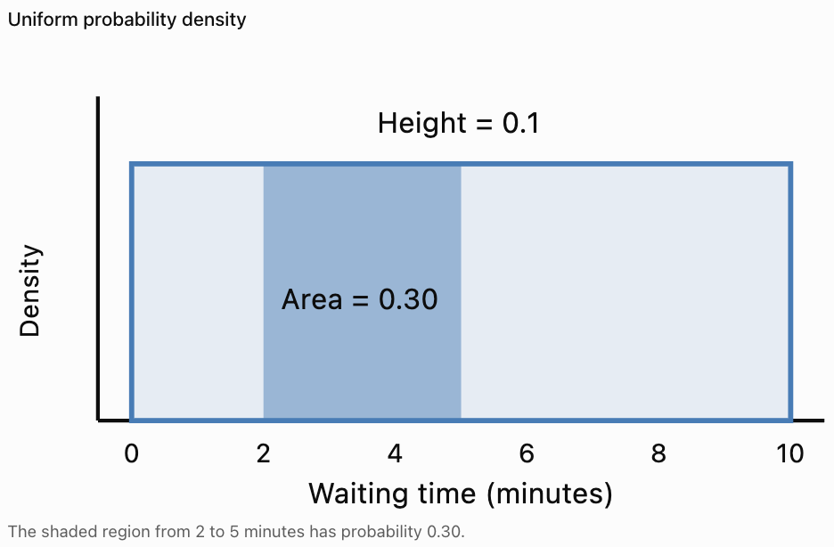
Suppose a bus arrives at a random time during a 10-minute interval.
Assume every arrival time within the interval is equally likely.
Let X represent the waiting time, in minutes.
X is uniformly distributed between 0 and 10.
Probability Density
The density is constant:
f(x) = 1/10, for 0 ≤ x ≤ 10
The total area is:
10 × 1/10 = 1
Worked Example
Find the probability that the waiting time is between 2 and 5 minutes.
Step 1: Identify the Interval Width
5 − 2 = 3 minutes
Step 2: Calculate the Area
P(2 ≤ X ≤ 5) = 3 × 1/10
P(2 ≤ X ≤ 5) = 0.30
Interpretation
There is a 30% probability that the waiting time lies between 2 and 5 minutes.
Expected Value of a Continuous Random Variable
The expected value of a continuous random variable is calculated using integration.
E(X) = ∫ x f(x) dx
The integral is taken over the possible values of X.
This is the continuous equivalent of multiplying each discrete value by its probability and adding.
Uniform Distribution Example
For a continuous uniform distribution between a and b:
E(X) = (a + b)/2
If a waiting time is uniformly distributed between 0 and 10 minutes:
E(X) = (0 + 10)/2
E(X) = 5 minutes
Interpretation
The expected waiting time is five minutes.
An individual passenger may wait more or less than five minutes.
Probability Distributions and Graphs
Different random variables are represented using different types of graphs.
Discrete Probability Distribution
A discrete probability distribution is commonly represented using separate bars.
The height of each bar represents the probability of an individual value.
Continuous Probability Distribution
A continuous probability distribution is represented using a density curve.
The area under the curve over an interval represents probability.
Important Distinction
For discrete variables, probabilities can be associated with individual values.
For continuous variables, probabilities are associated with intervals.


Variance and Standard Deviation of Random Variables
Expected value describes the centre of a probability distribution.
However, two random variables can have the same expected value and different levels of variability.
Variance and standard deviation measure how spread out the possible values are around the expected value.
Variance of a Discrete Random Variable
Var(X) = Σ[(x − μ)²P(X = x)]
where:
μ = E(X)
An equivalent formula is:
Var(X) = E(X²) − [E(X)]²
Standard Deviation
σ = √Var(X)
Worked Example
Consider:
|
X |
Probability |
|---|---|
|
0 |
0.25 |
|
1 |
0.50 |
|
2 |
0.25 |
We previously found:
E(X) = 1
Calculate E(X²):
E(X²) = 0²(0.25) + 1²(0.50) + 2²(0.25)
E(X²) = 0 + 0.50 + 1
E(X²) = 1.5
Therefore:
Var(X) = 1.5 − 1²
Var(X) = 0.5
Standard deviation:
σ = √0.5
σ ≈ 0.707
Interpretation
The expected value is 1.
The standard deviation is approximately 0.707.
This describes the spread of the possible outcomes around the expected value.
Transforming Random Variables
Sometimes a random variable is multiplied by a constant or increased by a fixed amount.
Suppose:
Y = aX + b
where a and b are constants.
The expected value follows:
E(Y) = aE(X) + b
Worked Example
A worker earns $15 for each item completed, plus a fixed daily payment of $20.
Let X represent the number of items completed.
Suppose:
E(X) = 8
The worker's daily earnings are:
Y = 15X + 20
Calculate the expected earnings:
E(Y) = 15E(X) + 20
E(Y) = 15(8) + 20
E(Y) = $140
Important Observation
Expected value can be used to predict average earnings, costs, or other quantities when they are calculated from a random variable.
Real-World Application: Insurance
Insurance companies use probability models to estimate expected claims.

Example
Suppose an insurance company estimates that a particular type of claim has:
-
A 2% probability of occurring during a year.
-
An average payment of $5,000 if it occurs.
In this simplified model, assume the payment is exactly $5,000 when a claim occurs.
Let X represent the claim payment.
|
X |
Probability |
|---|---|
|
$0 |
0.98 |
|
$5,000 |
0.02 |
Expected claim payment:
E(X) = 0(0.98) + 5,000(0.02)
E(X) = $100
Interpretation
The expected claim payment is $100 per policy per year.
Actual insurance premiums may be higher because they also account for administration, uncertainty, capital requirements, and other costs.
Real-World Application: Scientific Experiments
Scientists often use random variables to represent uncertain experimental outcomes.
Examples include:
-
Number of radioactive decays during a time interval.
-
Number of particles detected.
-
Measurement errors.
-
Time between events.
-
Number of successful trials.

Example
A detector records the number of particles arriving during one minute.
Let X represent the number of detected particles.
X is discrete because it counts individual particles.
If instead we measure the time between detections, that waiting time can be modelled as continuous.
This demonstrates how closely related scientific measurements can involve different types of random variables.
Real-World Application: Weather
Weather predictions frequently involve probability distributions.
For example:
-
Amount of rainfall.
-
Daily maximum temperature.
-
Wind speed.
-
Number of thunderstorms.
-
Time until the next rainfall event.

Example
Let X represent the number of thunderstorms occurring during a day.
X is discrete.
Let Y represent the amount of rainfall in millimetres.
Y is continuous in a measurement model, although recorded values may be rounded.
Interpretation
Random variables allow meteorologists to describe uncertainty rather than predict only a single value.
Probability distributions can provide information about both typical conditions and the likelihood of unusual events.
Common Mistakes
Confusing an outcome with a random variable
An outcome describes what happens. A random variable assigns a numerical value to that outcome.
Assuming every random variable is continuous
Counts are usually discrete.
Assuming every random variable is discrete
Measurements are often modelled as continuous.
Forgetting that probabilities must add to 1
A discrete probability distribution must have total probability 1.
Using probabilities greater than 1
Probabilities must lie between 0 and 1.
Forgetting to multiply values by their probabilities
Expected value is a weighted average, not necessarily the ordinary average of the possible values.
Assuming expected value must be a possible outcome
Expected values can be fractional even when the random variable counts whole objects.
Confusing expected prize with expected net gain
Net gain must account for the cost of participating.
Assuming expected value predicts an individual result
Expected value describes a long-run average.
Confusing probability density with probability
For continuous distributions, probability is represented by area under the density curve.
Assuming an exact continuous value has positive probability
Under a continuous probability model, the probability of any single exact value is zero.
Ignoring the conditions of a probability model
Assumptions such as independence, constant probabilities, and fairness must be appropriate.
Key Terms
-
Random Experiment: Process with uncertain outcomes.
-
Outcome: Possible result of a random experiment.
-
Sample Space: Set of all possible outcomes.
-
Random Variable: Function assigning numerical values to outcomes.
-
Discrete Random Variable: Random variable with finite or countably infinite possible values.
-
Continuous Random Variable: Random variable taking values across continuous intervals.
-
Probability Distribution: Description of possible values and their probabilities.
-
Probability Mass Function: Function giving probabilities of individual discrete values.
-
Probability Density Function: Function whose area over an interval gives continuous probability.
-
Cumulative Distribution Function: Function giving P(X ≤ x).
-
Expected Value: Probability-weighted average of a random variable.
-
Mean of a Random Variable: Another name for its expected value.
-
Variance: Measure of the spread of a probability distribution.
-
Standard Deviation: Square root of variance.
-
Probability: Numerical measure of the likelihood of an event.
-
Independent Events: Events whose occurrence does not affect each other's probabilities.
-
Fair Game: Game with an expected net gain of zero.
-
Net Gain: Winnings minus costs.
-
Long-Run Average: Average approached over many repetitions under stable conditions.
-
Binomial Distribution: Distribution describing successes in a fixed number of independent trials with constant success probability.
-
Uniform Distribution: Distribution with equal probabilities for discrete values or constant density across a continuous interval.
-
Probability Model: Mathematical representation of uncertainty.
-
Weighted Average: Average accounting for the relative importance or probability of each value.
-
Cumulative Probability: Probability that a variable is at or below a specified value.
Key Takeaways
-
A random variable assigns numerical values to outcomes of a random experiment.
-
Random variables may be discrete or continuous.
-
Discrete random variables often involve counting.
-
Continuous random variables often involve measurement.
-
A probability distribution describes possible values and their probabilities.
-
All probabilities in a discrete distribution must be between 0 and 1.
-
The probabilities of all possible discrete values must add to 1.
-
Expected value is a probability-weighted average.
-
For a discrete variable, E(X) = Σ[x × P(X = x)].
-
Expected value does not need to be a possible individual outcome.
-
Expected value is useful for analysing games, business decisions, insurance, and scientific experiments.
-
A fair game has an expected net gain of zero.
-
For continuous variables, probabilities correspond to areas under density curves.
-
The total area under a probability density curve is 1.
-
Variance and standard deviation describe the spread of a random variable.
-
Random variables provide mathematical tools for making decisions under uncertainty.
Check Your Understanding
Random Variables
-
Define a random variable.
-
Explain the difference between a discrete and continuous random variable.
-
Is the number of students absent from school discrete or continuous?
-
Is the height of a student discrete or continuous?
-
Is the time required to complete an examination discrete or continuous?
Probability Distributions
-
State the two requirements of a valid discrete probability distribution.
-
Determine whether probabilities 0.20, 0.30, 0.40, and 0.10 form a valid distribution.
-
Determine whether probabilities 0.25, 0.35, 0.50, and 0.20 form a valid distribution.
-
A random variable has P(X = 0) = 0.2, P(X = 1) = 0.5, and P(X = 2) = 0.3. Find P(X ≥ 1).
-
For the same distribution, find P(X ≤ 1).
Expected Value
-
Calculate the expected value of a fair six-sided die.
-
Calculate E(X) for X = 0, 1, 2 with probabilities 0.2, 0.5, 0.3.
-
Explain why expected value does not have to be a possible outcome.
-
A game costs $2. A player has a 1/4 chance of winning $8 and otherwise wins nothing. Find the expected net gain.
-
A basketball player has an 80% chance of making each free throw. Find the expected number of successful shots in 15 independent attempts.
Continuous Random Variables
-
What does the area under a probability density curve represent?
-
What is the total area under a valid probability density curve?
-
Why is P(X = 5) = 0 for a continuous random variable?
-
A waiting time is uniformly distributed between 0 and 20 minutes. Find the probability of waiting between 5 and 10 minutes.
-
Find the expected waiting time for the same uniform distribution.
Answer Key
|
Question |
Answer |
|---|---|
|
1 |
Function assigning numerical values to random outcomes |
|
2 |
Discrete values are countable; continuous values lie across intervals |
|
3 |
Discrete |
|
4 |
Continuous |
|
5 |
Continuous |
|
6 |
Each probability is between 0 and 1; total probability is 1 |
|
7 |
Yes |
|
8 |
No; total = 1.30 |
|
9 |
0.80 |
|
10 |
0.70 |
|
11 |
3.5 |
|
12 |
1.1 |
|
13 |
It represents a weighted long-run average |
|
14 |
$0 |
|
15 |
12 |
|
16 |
Probability over an interval |
|
17 |
1 |
|
18 |
A single point has zero area |
|
19 |
0.25 |
|
20 |
10 minutes |
Extended Challenge
Classifying Random Variables
-
Classify the number of books borrowed from a library during a day.
-
Classify the mass of a randomly selected apple.
-
Classify the number of customers arriving at a shop.
-
Classify the temperature of a classroom.
-
Explain why the number of rainfall events and the amount of rainfall are different types of random variables.
Constructing Distributions
-
Construct the probability distribution for the number of heads in three fair coin tosses.
-
Verify that the probabilities add to 1.
-
Calculate the expected number of heads.
-
Find the probability of obtaining at least two heads.
-
Find the probability of obtaining fewer than two heads.
Expected Value Applications
-
A game awards $10 with probability 0.2 and nothing otherwise. Calculate the expected prize.
-
If the game costs $3, calculate the expected net gain.
-
A company sells 0, 1, 2, or 3 products with probabilities 0.1, 0.2, 0.4, and 0.3. Find the expected number sold.
-
Each product earns $25 in profit. Find the expected daily profit.
-
Explain why a business might prefer a decision with lower expected profit but less uncertainty.
Continuous Distributions
-
A waiting time is uniformly distributed between 0 and 30 minutes. Find P(10 ≤ X ≤ 20).
-
Find the expected waiting time.
-
Explain why the probability of waiting exactly 15 minutes is zero in the continuous model.
-
Explain how a probability density function differs from a discrete probability mass function.
-
Describe a real-world situation in which a continuous probability distribution would be useful.
Final Investigation: Designing a Probability Game
You are designing a game using a fair six-sided die.
The game costs $4 to play.
Players receive prizes according to the following rules:
-
Rolling a 1 or 2 wins nothing.
-
Rolling a 3 or 4 wins $3.
-
Rolling a 5 wins $6.
-
Rolling a 6 wins $12.
Complete the investigation.
-
Define a random variable X representing the prize awarded.
-
List all possible values of X.
-
Calculate the probability of each prize.
-
Construct a probability distribution table.
-
Verify that the probabilities add to 1.
-
Construct a bar graph of the distribution.
-
Calculate the expected prize.
-
Calculate the expected net gain after paying the $4 entry fee.
-
Determine whether the game is fair.
-
Explain whether the game favours the player or the organiser.
-
Calculate the probability of winning any prize.
-
Calculate the probability of winning more than the entry fee.
-
Calculate the probability of losing money.
-
Calculate the probability of breaking even.
-
Determine the expected total net gain for a player over 100 games.
-
Explain why the actual results of 100 games may differ from the expected result.
-
Determine an entry fee that would make the game fair.
-
Suggest a change to one prize that would make the game fair while keeping the $4 entry fee.
-
Explain how probability distributions can help people evaluate games of chance.
-
Write a conclusion describing the role of expected value in financial decision-making.
2. Binomial Distribution
Learning outcomes
- I can identify binomial experiments.
- I can calculate binomial probabilities.
- I can determine expected values.
- I can calculate variance and standard deviation.
- I can solve practical problems involving binomial distributions.
Binomial Distribution
Introduction
Many situations involve repeating an experiment and counting how many times a particular result occurs.
For example:
-
How many heads will appear when a coin is tossed ten times?
-
How many basketball free throws will a player make out of eight attempts?
-
How many defective products will be found in a sample of twenty?
-
How many students will answer a multiple-choice question correctly?
-
How many seeds will germinate when ten seeds are planted?
These situations can often be modelled using the binomial distribution.
The binomial distribution is a discrete probability distribution that describes the number of successes in a fixed number of independent trials, where each trial has two possible outcomes and the probability of success remains constant.
It allows us to calculate probabilities, expected values, variance, and standard deviation.


What Is a Binomial Experiment?
A binomial experiment is a probability experiment that satisfies four important conditions.
These conditions can be remembered using the acronym BINS.
|
Letter |
Condition |
Meaning |
|---|---|---|
|
B |
Binary outcomes |
Each trial has two possible outcomes |
|
I |
Independent trials |
One trial does not affect another |
|
N |
Number of trials fixed |
The total number of trials is known |
|
S |
Same probability |
Probability of success remains constant |
All four conditions must be satisfied for the standard binomial model to apply.
Binary Outcomes
Each trial must have two possible outcomes, usually called:
-
Success
-
Failure
Success does not necessarily mean something positive.
For example, if a factory is counting defective products, finding a defective product may be defined as a success.
Independent Trials
The result of one trial must not change the probability of success on another trial.
For example, tossing a fair coin repeatedly produces independent results.
However, drawing cards from a deck without replacement generally produces dependent results.
Fixed Number of Trials
The experiment must have a predetermined number of trials.
For example, tossing a coin exactly ten times satisfies this condition.
Tossing a coin until the first head appears does not have a fixed number of trials.
Constant Probability
The probability of success must remain the same on every trial.
For a fair coin:
p = 0.5
For a fair die, if success means rolling a 6:
p = 1/6
Identifying Binomial Experiments
Consider the following situations.
|
Situation |
Binomial? |
Explanation |
|---|---|---|
|
Tossing a fair coin ten times and counting heads |
Yes |
All four conditions satisfied |
|
Rolling a fair die eight times and counting sixes |
Yes |
Success or failure on each independent roll |
|
Measuring the heights of twenty students |
No |
Height is continuous, not binary |
|
Drawing five cards without replacement and counting aces |
Not exactly |
Success probability changes |
|
Taking ten independent free throws with constant success probability |
Yes |
Fixed independent binary trials |
|
Tossing a coin until the first head appears |
No |
Number of trials is not fixed |
Important Observation
A trial may originally have more than two possible outcomes but still be classified into success and failure.
For example, a die has six possible outcomes.
However, if success means rolling a 6, the outcomes can be grouped as:
Success: 6
Failure: 1, 2, 3, 4, or 5
This produces a valid binary classification.
Binomial Random Variables
A binomial random variable counts the number of successes in a binomial experiment.
Let:
-
X = number of successes
-
n = number of trials
-
p = probability of success
-
1 − p = probability of failure
The probability of failure is often represented by q.
q = 1 − p
A binomial random variable is written:
X ~ Bin(n, p)
This means X follows a binomial distribution with n trials and probability of success p.
Example
A fair coin is tossed five times.
Let X represent the number of heads.
Then:
n = 5
p = 0.5
X ~ Bin(5, 0.5)
The possible values of X are:
0, 1, 2, 3, 4, 5
Understanding the Binomial Distribution
The binomial distribution gives the probability of obtaining each possible number of successes.
For example, when four fair coins are tossed, there are five possible numbers of heads:
0, 1, 2, 3, or 4.
The probabilities are not all equal.
Obtaining exactly two heads is more likely than obtaining zero heads because there are more ways to arrange two heads among four tosses.
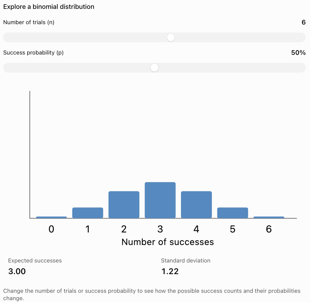
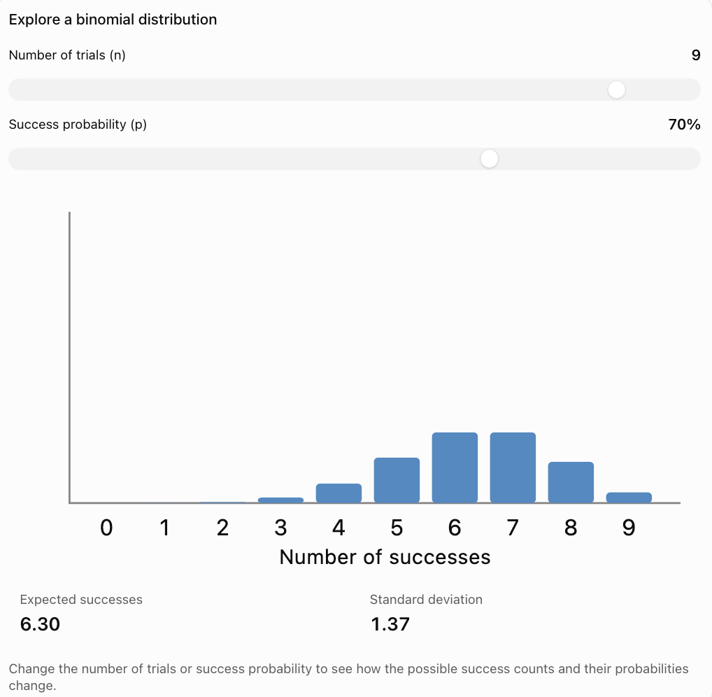
Explore how the distribution changes as the number of trials and probability of success change.
What Happens When p Changes?
When p = 0.5, the distribution is symmetric.
When p is less than 0.5, the distribution tends to be right-skewed.
When p is greater than 0.5, the distribution tends to be left-skewed.
As the number of trials increases, the distribution may begin to resemble a normal distribution, provided neither success nor failure is too rare.
The Binomial Probability Formula
The probability of obtaining exactly k successes in n independent trials is:
P(X = k) = C(n, k) × pᵏ × (1 − p)ⁿ⁻ᵏ
where:
-
n = number of trials
-
k = number of successes
-
p = probability of success
-
1 − p = probability of failure
-
C(n, k) = number of ways to choose k successes from n trials
The combination formula is:
C(n, k) = n! / [k!(n − k)!]
The symbol ! represents a factorial.
For example:
5! = 5 × 4 × 3 × 2 × 1 = 120
Also:
0! = 1
Why Does the Formula Work?
The expression:
pᵏ × (1 − p)ⁿ⁻ᵏ
gives the probability of one particular arrangement of k successes and n − k failures.
The expression:
C(n, k)
counts how many different arrangements are possible.
Multiplying them gives the total probability of obtaining exactly k successes.
Worked Example: Tossing Coins
A fair coin is tossed five times.
Find the probability of obtaining exactly three heads.
Step 1: Identify the Values
n = 5
k = 3
p = 0.5
Step 2: Calculate the Number of Combinations
C(5, 3) = 5! / (3!2!)
C(5, 3) = 10
Step 3: Substitute into the Formula
P(X = 3) = 10 × (0.5)³ × (0.5)²
P(X = 3) = 10 × 0.125 × 0.25
P(X = 3) = 0.3125
Final Answer
There is a 31.25% probability of obtaining exactly three heads in five tosses.
Interpretation
If this experiment were repeated many times, approximately 31.25% of the five-toss experiments would produce exactly three heads.
Worked Example: Rolling a Die
A fair six-sided die is rolled four times.
Find the probability of rolling exactly two sixes.
Step 1: Identify the Values
n = 4
k = 2
p = 1/6
1 − p = 5/6
Step 2: Calculate the Combinations
C(4, 2) = 6
Step 3: Apply the Formula
P(X = 2) = 6 × (1/6)² × (5/6)²
P(X = 2) = 6 × (1/36) × (25/36)
P(X = 2) = 150/1296
P(X = 2) ≈ 0.1157
Final Answer
The probability of rolling exactly two sixes is approximately 11.57%.

Calculating Probabilities for Different Outcomes
A binomial distribution can be used to calculate probabilities involving:
-
Exactly k successes.
-
At least k successes.
-
At most k successes.
-
More than k successes.
-
Fewer than k successes.
These phrases are important because they determine which probabilities must be included.
|
Phrase |
Mathematical notation |
|---|---|
|
Exactly 3 |
P(X = 3) |
|
At least 3 |
P(X ≥ 3) |
|
At most 3 |
P(X ≤ 3) |
|
More than 3 |
P(X > 3) |
|
Fewer than 3 |
P(X < 3) |
Calculating At Least a Certain Number of Successes
Suppose a basketball player has an 80% probability of making a free throw.
The player takes five independent shots.
Find the probability of making at least four shots.
Step 1: Identify the Values
n = 5
p = 0.8
We need:
P(X ≥ 4)
Step 2: Identify the Included Outcomes
P(X ≥ 4) = P(X = 4) + P(X = 5)
Step 3: Calculate P(X = 4)
P(X = 4) = C(5, 4)(0.8)⁴(0.2)¹
= 5 × 0.4096 × 0.2
= 0.4096
Step 4: Calculate P(X = 5)
P(X = 5) = C(5, 5)(0.8)⁵
= 0.32768
Step 5: Add
P(X ≥ 4) = 0.4096 + 0.32768
P(X ≥ 4) = 0.73728
Final Answer
There is approximately a 73.73% probability of making at least four out of five shots.
Using Complementary Probability
Sometimes it is easier to calculate the probability of the opposite event.
The complement rule is:
P(A) = 1 − P(not A)
Example: At Least One Success
A fair coin is tossed six times.
Find the probability of obtaining at least one head.
Instead of calculating the probabilities for one, two, three, four, five, and six heads, calculate the probability of no heads.
Step 1: Calculate P(X = 0)
P(X = 0) = (0.5)⁶
P(X = 0) = 0.015625
Step 2: Apply the Complement Rule
P(X ≥ 1) = 1 − P(X = 0)
P(X ≥ 1) = 1 − 0.015625
P(X ≥ 1) = 0.984375
Final Answer
There is a 98.4375% probability of obtaining at least one head in six fair coin tosses.
When Is the Complement Rule Useful?
The complement rule is especially useful for questions involving:
-
At least one success.
-
At least one failure.
-
More than a specified number.
-
Fewer than a specified number.
It can greatly reduce the number of calculations.
Expected Value of a Binomial Distribution
The expected value represents the average number of successes expected over many repetitions of the experiment.
For a binomial distribution:
E(X) = np
where:
n = number of trials
p = probability of success
Worked Example
A student guesses on ten multiple-choice questions.
Each question has four options, with one correct answer.
Assume the guesses are independent.
Step 1: Identify the Values
n = 10
p = 1/4 = 0.25
Step 2: Calculate the Expected Value
E(X) = 10 × 0.25
E(X) = 2.5
Interpretation
The student is expected to answer an average of 2.5 questions correctly.
This does not mean the student can answer half a question correctly.
It represents the average number of correct answers across many sets of ten guesses.
Variance of a Binomial Distribution
The variance measures the spread of the number of successes around its expected value.
For a binomial distribution:
Var(X) = np(1 − p)
Since q = 1 − p, the formula may also be written:
Var(X) = npq
Worked Example
A fair coin is tossed twenty times.
Find the variance of the number of heads.
Step 1: Identify the Values
n = 20
p = 0.5
q = 0.5
Step 2: Calculate
Var(X) = 20 × 0.5 × 0.5
Var(X) = 5
Interpretation
The variance describes the spread of the possible numbers of heads around the expected value of 10.
Variance is measured in squared units, which is why standard deviation is often easier to interpret.
Standard Deviation of a Binomial Distribution
The standard deviation is the square root of the variance.
For a binomial distribution:
σ = √[np(1 − p)]
Worked Example
A fair coin is tossed twenty times.
We previously calculated:
Var(X) = 5
Therefore:
σ = √5
σ ≈ 2.24
Interpretation
The number of heads typically varies by an amount on the order of 2.24 from the expected value of 10.
This does not mean that every experiment will produce between 7.76 and 12.24 heads.
Standard deviation measures variability, not a guaranteed interval.
Combining Mean, Variance, and Standard Deviation
Suppose a factory produces items with a 5% probability of being defective.
A sample of 100 items is inspected.
Assume defects occur independently and the defect probability remains constant.
Let X represent the number of defective items.
Step 1: Identify the Distribution
n = 100
p = 0.05
X ~ Bin(100, 0.05)
Step 2: Calculate Expected Value
E(X) = np
E(X) = 100 × 0.05
E(X) = 5
Step 3: Calculate Variance
Var(X) = np(1 − p)
Var(X) = 100 × 0.05 × 0.95
Var(X) = 4.75
Step 4: Calculate Standard Deviation
σ = √4.75
σ ≈ 2.18
Interpretation
The factory expects approximately five defective items per sample of 100.
The standard deviation is approximately 2.18 defective items.
The actual number of defective items will vary between samples.
Understanding How n and p Affect the Distribution
The shape and spread of a binomial distribution depend on n and p.
Effect of Increasing n
When p remains constant and n increases:
-
The expected number of successes increases.
-
The variance increases.
-
The standard deviation increases.
-
The relative variation, measured as a fraction of n, generally decreases for 0 < p < 1.
Effect of Changing p
When n remains constant:
-
Small p values concentrate probability near zero successes.
-
Large p values concentrate probability near n successes.
-
p = 0.5 produces a symmetric distribution.
-
Variance is largest when p = 0.5.
Example
For n = 10:
|
p |
Expected value |
Variance |
Standard deviation |
|---|---|---|---|
|
0.1 |
1 |
0.9 |
0.95 |
|
0.3 |
3 |
2.1 |
1.45 |
|
0.5 |
5 |
2.5 |
1.58 |
|
0.7 |
7 |
2.1 |
1.45 |
|
0.9 |
9 |
0.9 |
0.95 |
The distribution has the greatest variance when success and failure are equally likely.
Binomial Distribution and the Normal Approximation
For sufficiently large n, a binomial distribution can often be approximated using a normal distribution.
A common guideline is:
np ≥ 10
and
n(1 − p) ≥ 10
These conditions help ensure that the distribution is not excessively skewed.
Example
Suppose:
n = 100
p = 0.5
Then:
np = 50
n(1 − p) = 50
Both values exceed 10.
A normal approximation may be appropriate.
Mean and Standard Deviation
The approximating normal distribution has:
Mean = np
Standard deviation = √[np(1 − p)]
Continuity Correction
Because a binomial random variable is discrete and the normal distribution is continuous, a continuity correction can improve the approximation.
For example:
P(X ≤ 20)
is approximated using:
P(Y ≤ 20.5)
where Y is the corresponding normal random variable.
This is an extension of the basic binomial model.
Real-World Application: Manufacturing Quality Control
Manufacturers use binomial probability models to analyse defective products.

Example
A factory estimates that 3% of its products are defective.
A quality-control inspector randomly selects twenty products.
Assume independent outcomes with constant defect probability.
Let X represent the number of defective products.
X ~ Bin(20, 0.03)
Expected Number of Defects
E(X) = 20 × 0.03
E(X) = 0.6
Probability of No Defects
P(X = 0) = (0.97)²⁰
P(X = 0) ≈ 0.5438
Interpretation
There is approximately a 54.38% probability that none of the twenty selected products will be defective.
Although the expected number of defects is only 0.6, the sample may contain zero, one, or several defective items.
Real-World Application: Medical Testing
Binomial distributions can model the number of positive test results under suitable assumptions.

Example
Suppose a screening programme tests 50 independent samples.
Assume each sample has a 10% probability of testing positive.
Let X represent the number of positive results.
X ~ Bin(50, 0.10)
Expected Value
E(X) = 50 × 0.10
E(X) = 5
Variance
Var(X) = 50 × 0.10 × 0.90
Var(X) = 4.5
Standard Deviation
σ = √4.5
σ ≈ 2.12
Interpretation
The expected number of positive results is five.
The actual number may vary between samples.
In real medical testing, independence and constant probability may not always be appropriate. Test accuracy and the population being tested also matter.
Real-World Application: Sports Performance
Binomial models can help analyse repeated sports attempts.

Example
A basketball player makes 75% of free throws.
Assume independent attempts with a constant success probability.
The player takes eight shots.
Find the probability of making exactly six.
Step 1: Identify the Values
n = 8
p = 0.75
k = 6
Step 2: Apply the Formula
P(X = 6) = C(8, 6)(0.75)⁶(0.25)²
C(8, 6) = 28
P(X = 6) = 28 × 0.1779785 × 0.0625
P(X = 6) ≈ 0.3115
Final Answer
There is approximately a 31.15% probability of making exactly six out of eight free throws.
Real-World Application: Education
Teachers can use binomial probability to investigate guessing on multiple-choice examinations.
Example
A student guesses randomly on twelve questions.
Each question has four options, with one correct answer.
Assume independent guesses.
Distribution
n = 12
p = 0.25
X ~ Bin(12, 0.25)
Expected Correct Answers
E(X) = 12 × 0.25
E(X) = 3
Probability of Getting All Questions Wrong
P(X = 0) = (0.75)¹²
P(X = 0) ≈ 0.0317
Interpretation
There is approximately a 3.17% probability of getting every question wrong through random guessing.
The expected number of correct answers is three.
Common Mistakes
Assuming every repeated experiment is binomial
All four BINS conditions must be satisfied.
Forgetting that trials must be independent
Dependent trials may require a different probability model.
Using the wrong success probability
The value of p must correspond to the event defined as success.
Confusing n and k
n is the total number of trials.
k is the number of successes.
Forgetting the combination term
C(n, k) counts the possible arrangements of successes.
Using p instead of 1 − p for failures
The failure probability is q = 1 − p.
Confusing exactly with at least
Exactly three means X = 3.
At least three means X ≥ 3.
Adding probabilities incorrectly
Events representing different possible numbers of successes must be combined correctly.
Forgetting the complement rule
Sometimes calculating the opposite event is much easier.
Confusing expected value with probability
Expected value is a number of successes, not a probability.
Using the wrong variance formula
Variance = np(1 − p), not np.
Forgetting the square root for standard deviation
Standard deviation = √[np(1 − p)].
Assuming expected value must be a whole number
Expected value may be fractional.
Applying a normal approximation without checking conditions
The approximation may be inaccurate when n is small or p is close to 0 or 1.
Key Terms
-
Binomial Experiment: Experiment with a fixed number of independent binary trials and constant success probability.
-
Binomial Distribution: Discrete probability distribution describing the number of successes in a binomial experiment.
-
Trial: Single repetition of an experiment.
-
Success: Outcome designated as the event of interest.
-
Failure: Outcome that is not classified as success.
-
Independent Trials: Trials whose outcomes do not affect one another's probabilities.
-
Probability of Success (p): Probability that a trial produces a success.
-
Probability of Failure (q): Probability that a trial produces a failure, where q = 1 − p.
-
Number of Trials
: Total number of repetitions.
-
Number of Successes (k): Number of successful outcomes.
-
Combination: Number of ways to select objects or positions without regard to order.
-
Factorial: Product of positive integers from 1 to a specified integer.
-
Binomial Coefficient: Number C(n, k) of ways to choose k successes from n trials.
-
Probability Mass Function: Function assigning probabilities to discrete values.
-
Expected Value: Long-run average number of successes.
-
Variance: Measure of the spread of the distribution around its mean.
-
Standard Deviation: Square root of variance.
-
Complementary Probability: Probability of an event not occurring.
-
Cumulative Probability: Probability of obtaining at most a specified number of successes.
-
Symmetric Distribution: Distribution with balanced left and right sides.
-
Skewed Distribution: Distribution with an extended tail on one side.
-
Normal Approximation: Use of a normal distribution to approximate a binomial distribution.
-
Continuity Correction: Adjustment used when approximating discrete probabilities with a continuous distribution.
Key Takeaways
-
Binomial experiments satisfy the four BINS conditions.
-
Each trial has two possible outcomes: success or failure.
-
The number of trials must be fixed.
-
Trials must be independent.
-
The probability of success must remain constant.
-
A binomial random variable counts the number of successes.
-
Binomial notation is X ~ Bin(n, p).
-
The binomial probability formula is P(X = k) = C(n, k)pᵏ(1 − p)ⁿ⁻ᵏ.
-
The expected value is E(X) = np.
-
The variance is Var(X) = np(1 − p).
-
The standard deviation is σ = √[np(1 − p)].
-
The complement rule simplifies many probability calculations.
-
A binomial distribution is symmetric when p = 0.5.
-
The distribution becomes increasingly skewed as p moves toward 0 or 1.
-
Binomial models are useful in manufacturing, medicine, sports, education, and scientific research.
-
The model should only be used when its assumptions are appropriate.
Check Your Understanding
Identifying Binomial Experiments
-
State the four conditions required for a binomial experiment.
-
Explain why tossing a fair coin ten times is binomial.
-
Explain why drawing cards without replacement is generally not exactly binomial.
-
Is counting the number of sixes in eight independent die rolls binomial?
-
Is measuring the heights of twenty students binomial?
Calculating Binomial Probabilities
-
Write the binomial probability formula.
-
Calculate C(5, 2).
-
A fair coin is tossed four times. Find P(X = 2).
-
A fair die is rolled three times. Find the probability of obtaining no sixes.
-
A player has a 60% probability of success. Find the probability of exactly two successes in three independent attempts.
Expected Value
-
Calculate E(X) for n = 20 and p = 0.4.
-
Calculate E(X) for n = 50 and p = 0.1.
-
Explain why the expected value may not be a whole number.
-
A student guesses on 16 four-option multiple-choice questions. Find the expected number correct.
-
A factory has a 2% defect rate. Find the expected number of defects in 200 independently produced items.
Variance and Standard Deviation
-
Write the formula for binomial variance.
-
Calculate the variance for n = 10 and p = 0.5.
-
Calculate the standard deviation for n = 10 and p = 0.5.
-
Calculate the variance for n = 40 and p = 0.2.
-
Explain what standard deviation tells us about a binomial distribution.
Answer Key
|
Question |
Answer |
|---|---|
|
1 |
Binary outcomes, independence, fixed n, constant p |
|
2 |
All four conditions are satisfied |
|
3 |
Probabilities change after cards are removed |
|
4 |
Yes |
|
5 |
No |
|
6 |
P(X = k) = C(n, k)pᵏ(1 − p)ⁿ⁻ᵏ |
|
7 |
10 |
|
8 |
0.375 |
|
9 |
(5/6)³ ≈ 0.5787 |
|
10 |
0.432 |
|
11 |
8 |
|
12 |
5 |
|
13 |
It is a long-run average |
|
14 |
4 |
|
15 |
4 |
|
16 |
Var(X) = np(1 − p) |
|
17 |
2.5 |
|
18 |
Approximately 1.58 |
|
19 |
6.4 |
|
20 |
It measures the spread of success counts around the expected value |
Extended Challenge
Binomial Identification
-
A student tosses a coin until the first head appears. Explain why this is not a binomial experiment.
-
A factory inspects twenty products selected independently from a very large production process. Explain when a binomial model would be appropriate.
-
A basketball player attempts ten free throws. Discuss the assumptions needed to use a binomial model.
-
Explain why rolling a die can produce a binomial experiment even though a die has six possible outcomes.
-
Describe a real-world experiment that satisfies all four BINS conditions.
Probability Calculations
-
A fair coin is tossed eight times. Find the probability of exactly five heads.
-
A fair die is rolled six times. Find the probability of exactly two sixes.
-
A player has a 70% success rate. Find the probability of exactly four successes in six independent attempts.
-
A factory has a 4% defect rate. Find the probability of no defective items in a sample of fifteen independent items.
-
A student guesses on ten four-option multiple-choice questions. Find the probability of answering at least one correctly.
Expected Value and Variability
-
Calculate the expected value for n = 60 and p = 0.3.
-
Calculate the variance for the same distribution.
-
Calculate the standard deviation.
-
Explain what happens to expected value when n doubles but p remains constant.
-
Explain why variance is greatest when p = 0.5 for a fixed n.
Practical Applications
-
A hospital estimates that 8% of patients will require a particular follow-up appointment. Find the expected number requiring follow-up among 100 independent patients.
-
Calculate the variance and standard deviation for the same situation.
-
A football player has a 65% probability of scoring a penalty. Find the probability of scoring at least three out of four independent penalties.
-
Explain why a binomial model might not be appropriate if a player's success probability changes due to fatigue.
-
Describe how binomial probabilities can help businesses make decisions under uncertainty.
Final Investigation: Quality Control in a Factory
A factory produces electronic components.
The probability that a component is defective is 0.05.
A quality-control inspector randomly selects twenty components.
Assume the selected components have independent defect outcomes and the probability of a defect remains constant.
Let X represent the number of defective components.
Complete the investigation.
-
Explain why this situation can be modelled using a binomial distribution.
-
Identify n.
-
Identify p.
-
Identify q.
-
Write the binomial notation for X.
-
Calculate the probability of finding no defective components.
-
Calculate the probability of finding exactly one defective component.
-
Calculate the probability of finding exactly two defective components.
-
Calculate the probability of finding at least one defective component.
-
Calculate the probability of finding at most two defective components.
-
Calculate the expected number of defective components.
-
Calculate the variance.
-
Calculate the standard deviation.
-
Construct a probability distribution table for X = 0 through X = 5.
-
Construct a bar graph for these probabilities.
-
Describe the shape of the distribution.
-
Explain why the expected number of defective components is not necessarily the most likely observed number.
-
Discuss whether a normal approximation would be appropriate.
-
Explain how the factory could use this model to plan quality-control inspections.
-
Write a conclusion explaining the usefulness and limitations of the binomial distribution in manufacturing.
3. Normal Distribution
Learning outcomes
- I can describe the characteristics of the normal distribution.
- I can calculate probabilities using normal distributions.
- I can apply z-scores to normal distributions.
- I can interpret normal probability graphs.
- I can solve practical problems involving normal distributions.
Normal Distribution
Introduction
Many measurements in the real world tend to cluster around an average value, with fewer observations occurring far above or below that average.
For example, when measuring the heights of a large group of people of similar age, most measurements may be near the average height. Very short and very tall measurements are generally less common.
This pattern can often be described using the normal distribution.
The normal distribution is one of the most important probability distributions in mathematics and statistics. It is widely used in scientific research, education, manufacturing, medicine, economics, and quality control.
It allows us to calculate the probability of a measurement falling within a particular range, determine how unusual an observation is, and compare results from different datasets.


 wQI6-jisIRlogp3oymKZba5mnc9mXGz426qzidVhdFh8AoCnsn60YpqhbjarVIGv7XJ31I0VDKHkGZVTHx7MQX_6HuRMYXhVEz1MV2IZO4nyLW1YVDUUv_ER3huob9-2D4XDusoXD9SupJEHAarcur2UG8Ow8Y?purpose=inline" alt="Quality Control Training Certificate | Free & Fast Course">
What Is a Normal Distribution?
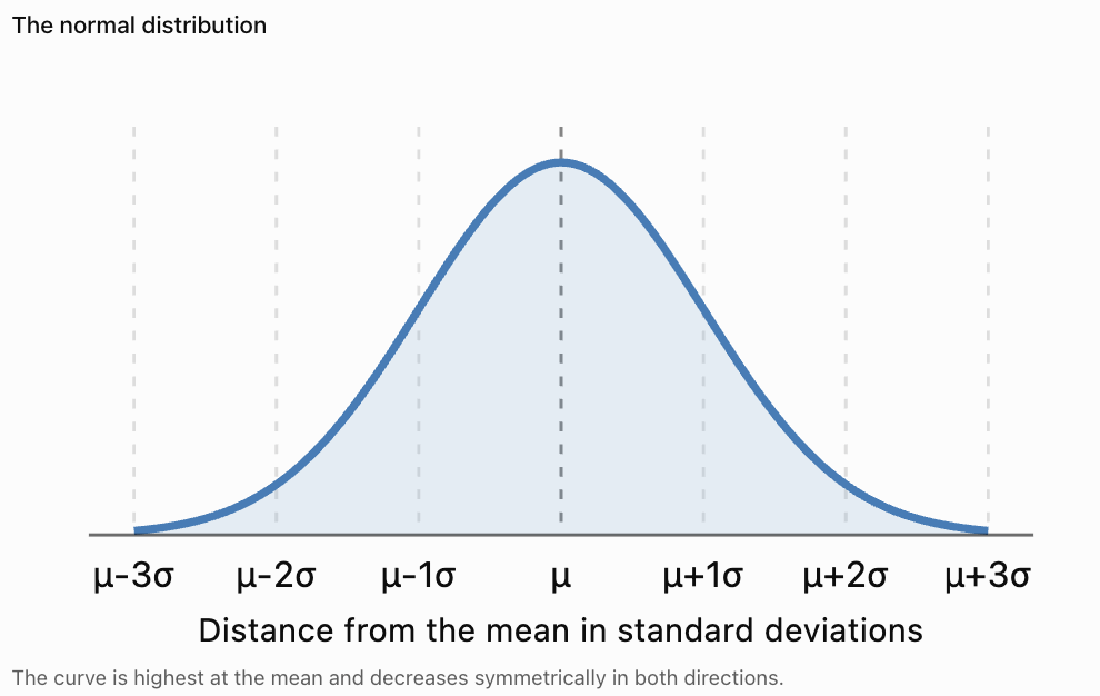
A normal distribution is a continuous probability distribution that is symmetric about its mean and has a characteristic bell-shaped curve.
The highest point of the curve occurs at the mean.
As values move farther from the mean, the probability density decreases.
Characteristics of the Normal Distribution
-
The distribution is symmetric about its mean.
-
It has one peak, making it unimodal.
-
The mean, median, and mode are equal.
-
The total area under the curve is 1.
-
The curve extends indefinitely in both directions.
-
The tails approach, but never touch, the horizontal axis.
-
Its shape is determined by the mean and standard deviation.
Important Observation
Not every bell-shaped dataset follows a perfectly normal distribution.
The normal distribution is a mathematical model. Real data may only approximate this shape.
The Mean and Standard Deviation
Two values completely determine a normal distribution.
Mean (μ)
The mean determines the centre of the distribution.
If the mean changes, the entire curve shifts left or right.
Standard Deviation (σ)
The standard deviation determines the spread of the distribution.
A smaller standard deviation produces a narrower, taller curve.
A larger standard deviation produces a wider, flatter curve.
Example
Consider two normally distributed examination results.
Statistic
Class A
Class B
Mean
70
70
Standard deviation
5
15
Both classes have the same average score.
However, Class A has less variation.
Most students in Class A score relatively close to 70.
Class B has a much wider spread of results.
Interpretation
The mean describes the centre.
The standard deviation describes the variability.
Both are needed to understand a normal distribution.
Notation for the Normal Distribution
A normal random variable is commonly written as:
X ~ N(μ, σ²)
where:
-
X = random variable
-
μ = population mean
-
σ² = population variance
-
σ = population standard deviation
Example
Suppose examination scores are normally distributed with:
Mean = 70
Standard deviation = 10
The variance is:
σ² = 10² = 100
Therefore:
X ~ N(70, 100)
Important Distinction
In this notation, the second parameter is the variance, not the standard deviation.
Some calculators ask for the mean and standard deviation separately, so always check the required inputs.
Understanding Area Under the Curve
The normal distribution is a continuous probability distribution.
For a continuous random variable, probability is represented by area under the curve.
The total area under the curve is:
1 or 100%
Example
Suppose X represents the height of a randomly selected person from a population whose heights are approximately normally distributed.
The probability that X lies between 160 cm and 180 cm is represented by the area under the curve between those two values.
Important Properties
For any continuous random variable:
P(X = a) = 0
This means the probability of obtaining one exact mathematical value is zero.
However, probabilities over intervals can be positive.
For example:
P(160 ≤ X ≤ 180)
may be substantial.
Why Does This Happen?
A single point has no width and therefore no area.
An interval has width, so the area under the curve can represent a nonzero probability.
The Empirical Rule
One of the most useful features of the normal distribution is the 68–95–99.7 rule.
This rule describes approximately how much of the distribution lies within one, two, and three standard deviations of the mean.
The empirical rule
68%
Within μ ± 1σ95%
Within μ ± 2σ99.7%
Within μ ± 3σWithin One Standard Deviation
Approximately 68% of observations lie between:
μ − σ and μ + σ
Within Two Standard Deviations
Approximately 95% of observations lie between:
μ − 2σ and μ + 2σ
Within Three Standard Deviations
Approximately 99.7% of observations lie between:
μ − 3σ and μ + 3σ
Example
Suppose examination scores have:
Mean = 70
Standard deviation = 10
Approximately:
-
68% of scores lie between 60 and 80.
-
95% lie between 50 and 90.
-
99.7% lie between 40 and 100.
These percentages assume a normal model. If scores are restricted to 0–100, an exact normal distribution is not possible, although a normal approximation may still be useful.
Understanding the Regions of a Normal Distribution
Because the normal distribution is symmetric, we can divide the empirical-rule percentages between the left and right sides.
Approximately:
Region
Percentage
Between μ and μ + σ
34%
Between μ + σ and μ + 2σ
13.5%
Between μ + 2σ and μ + 3σ
2.35%
Beyond μ + 3σ
0.15%
The same approximate percentages apply on the left side.
Worked Example
A normal distribution has mean 100 and standard deviation 15.
Estimate the percentage of observations between 100 and 115.
Since:
115 = μ + σ
The interval is from the mean to one standard deviation above the mean.
Approximately half of 68% lies in this interval.
Probability ≈ 34%
Interpretation
Approximately 34% of observations lie between 100 and 115.
The Standard Normal Distribution
The standard normal distribution is a special normal distribution with:
Mean = 0
Standard deviation = 1
It is written:
Z ~ N(0, 1)
The horizontal axis is measured in standard scores called z-scores.
Why Is It Useful?
Different normal distributions may have different means and standard deviations.
By converting observations into z-scores, we can use one standard normal distribution to calculate probabilities for all of them.
This process is called standardisation.
Calculating z-Scores
A z-score measures how many standard deviations an observation lies above or below the mean.
The formula is:
z = (x − μ)/σ
where:
-
z = standard score
-
x = observed value
-
μ = population mean
-
σ = population standard deviation
Interpretation
-
z = 0 means the observation equals the mean.
-
z = 1 means one standard deviation above the mean.
-
z = −1 means one standard deviation below the mean.
-
z = 2 means two standard deviations above the mean.
-
z = −2 means two standard deviations below the mean.
Worked Example
A normally distributed examination has:
Mean = 65
Standard deviation = 8
A student scores 81.
Calculate the z-score.
Step 1: Identify the Values
x = 81
μ = 65
σ = 8
Step 2: Substitute
z = (81 − 65)/8
z = 16/8
z = 2
Interpretation
The student scored two standard deviations above the mean.
This is a relatively high result compared with the reference distribution.
Calculating Negative z-Scores
A negative z-score indicates an observation below the mean.
Worked Example
A normal distribution has:
Mean = 50
Standard deviation = 6
An observation has value 41.
Calculate:
z = (41 − 50)/6
z = −9/6
z = −1.5
Interpretation
The observation is 1.5 standard deviations below the mean.
The negative sign describes its position relative to the mean.
It does not indicate that the original observation is negative.
Using Standard Normal Tables
A standard normal table provides probabilities associated with z-scores.
Most common z-tables give the cumulative probability:
P(Z ≤ z)
This represents the area under the standard normal curve to the left of z.
Common z-Scores and Probabilities
z-score
P(Z ≤ z)
−2.00
0.0228
−1.50
0.0668
−1.00
0.1587
−0.50
0.3085
0.00
0.5000
0.50
0.6915
1.00
0.8413
1.50
0.9332
2.00
0.9772
2.50
0.9938
3.00
0.9987
Important Observation
A z-table value is not the height of the curve.
It represents an area, or cumulative probability.
Calculating Probabilities Below a Value
Suppose:
X ~ N(70, 100)
This means:
Mean = 70
Standard deviation = 10
Find:
P(X < 85)
Step 1: Convert to a z-Score
z = (85 − 70)/10
z = 1.5
Step 2: Use the Standard Normal Table
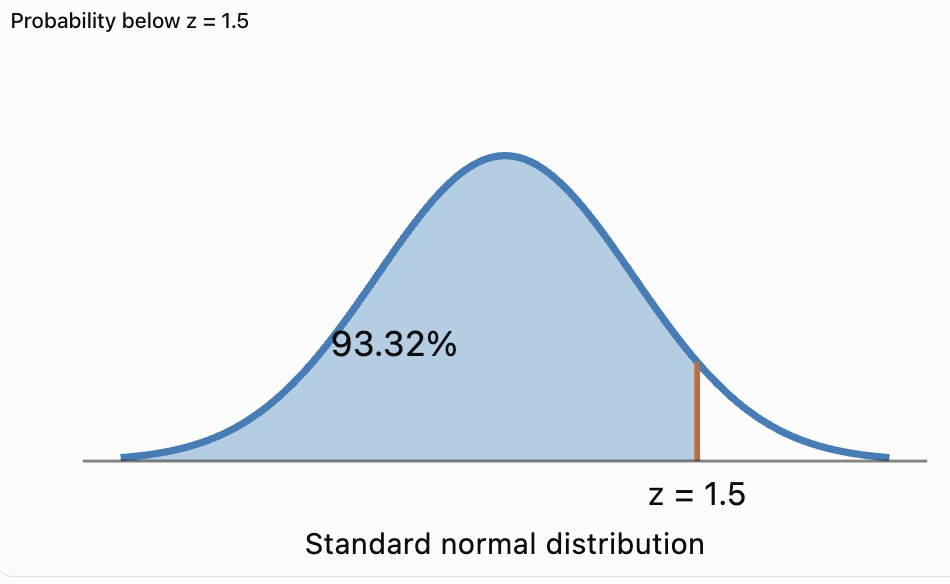
P(Z < 1.5) = 0.9332
Final Answer
P(X < 85) ≈ 0.9332
There is approximately a 93.32% probability that a randomly selected observation is below 85.
Graphical Interpretation
The area to the left of 85 represents approximately 93.32% of the distribution.
Calculating Probabilities Above a Value
Standard normal tables commonly provide the area to the left of a z-score.
To calculate the area to the right, use the complement rule.
P(Z > z) = 1 − P(Z ≤ z)
Worked Example
Suppose examination scores are normally distributed with:
Mean = 60
Standard deviation = 12
Find the probability that a student scores above 78.
Step 1: Calculate the z-Score
z = (78 − 60)/12
z = 1.5
Step 2: Find the Cumulative Probability
P(Z ≤ 1.5) = 0.9332
Step 3: Apply the Complement Rule
P(Z > 1.5) = 1 − 0.9332
P(Z > 1.5) = 0.0668
Final Answer
There is approximately a 6.68% probability of scoring above 78.
Calculating Probabilities Between Two Values
To calculate the probability between two values, subtract their cumulative probabilities.
P(a < X < b) = P(X < b) − P(X < a)
Worked Example
Suppose:
Mean = 100
Standard deviation = 15
Find the probability that X lies between 85 and 115.
Step 1: Calculate the Lower z-Score
z₁ = (85 − 100)/15
z₁ = −1
Step 2: Calculate the Upper z-Score
z₂ = (115 − 100)/15
z₂ = 1
Step 3: Find the Cumulative Probabilities
P(Z ≤ 1) = 0.8413
P(Z ≤ −1) = 0.1587
Step 4: Subtract
P(−1 < Z < 1) = 0.8413 − 0.1587
P(−1 < Z < 1) = 0.6826
Final Answer
There is approximately a 68.26% probability that X lies between 85 and 115.
This agrees with the empirical rule.
Using Symmetry to Calculate Probabilities
The normal distribution is symmetric around its mean.
Therefore:
P(Z < −a) = P(Z > a)
Example
Find:
P(Z < −2)
From the standard normal table:
P(Z < −2) = 0.0228
By symmetry:
P(Z > 2) = 0.0228
Interpretation
Approximately 2.28% of observations lie more than two standard deviations below the mean.
The same percentage lies more than two standard deviations above the mean.
Finding an Original Value from a z-Score
Sometimes we know the z-score and need to calculate the original measurement.
Start with:
z = (x − μ)/σ
Rearrange:
x = μ + zσ
Worked Example
A normal distribution has:
Mean = 75
Standard deviation = 12
Find the observation corresponding to z = 1.5.
Step 1: Substitute
x = 75 + 1.5(12)
x = 75 + 18
x = 93
Interpretation
An observation of 93 lies 1.5 standard deviations above the mean.
Finding Percentiles Using the Normal Distribution
Percentiles describe the relative position of observations within a distribution.
For a normal distribution, percentile values can be found using z-scores.
Common Percentiles
Percentile
Approximate z-score
5th
−1.645
10th
−1.282
25th
−0.674
50th
0
75th
0.674
90th
1.282
95th
1.645
97.5th
1.960
99th
2.326
Worked Example: Finding the 90th Percentile
Suppose examination scores are normally distributed with:
Mean = 70
Standard deviation = 10
Find the score corresponding to the 90th percentile.
Step 1: Identify the z-Score
The 90th percentile corresponds to approximately:
z = 1.282
Step 2: Use the Rearranged Formula
x = μ + zσ
x = 70 + 1.282(10)
x = 70 + 12.82
x ≈ 82.82
Interpretation
A score of approximately 82.8 is at the 90th percentile.
Approximately 90% of the distribution lies below this value.
Comparing Observations from Different Distributions
z-scores allow us to compare observations from normal distributions with different means and standard deviations.
Worked Example
Two students complete different examinations.
Statistic
Mathematics
Science
Student score
82
88
Mean
70
80
Standard deviation
8
10
Mathematics z-Score
z = (82 − 70)/8
z = 1.5
Science z-Score
z = (88 − 80)/10
z = 0.8
Interpretation
The Mathematics score is 1.5 standard deviations above its mean.
The Science score is 0.8 standard deviations above its mean.
The student performed better relative to the Mathematics reference group.
The higher raw Science score does not necessarily represent stronger relative performance.
Interpreting Normal Probability Graphs
Normal probability graphs communicate probabilities through shaded regions.
Left-Tail Probability
The shaded region extends from the far left to a specified value.
This represents:
P(X ≤ a)
Right-Tail Probability
The shaded region extends from a specified value to the far right.
This represents:
P(X ≥ a)
Central Probability
The shaded region lies between two values.
This represents:
P(a ≤ X ≤ b)
Two-Tail Probability
The shaded regions lie below one boundary and above another.
This may represent unusually low or unusually high observations.
7Important Observation
The area under the curve represents probability.
The height of the curve at a particular value represents probability density, not the probability of that exact value.
Real-World Application: Human Heights
Human height within a suitably defined population may be approximately normally distributed.
Example
Suppose adult heights in a reference population are modelled by a normal distribution with:
Mean = 170 cm
Standard deviation = 8 cm
Find the probability that a randomly selected adult is taller than 186 cm.
Step 1: Calculate the z-Score
z = (186 − 170)/8
z = 2
Step 2: Find the Right-Tail Probability
P(Z > 2) = 1 − 0.9772
P(Z > 2) = 0.0228
Interpretation
Approximately 2.28% of adults in the modelled population are taller than 186 cm.
The result depends on whether the chosen normal model accurately represents that population.
Real-World Application: Manufacturing Quality Control
Factories use normal distributions to monitor product measurements.
Example
A factory produces metal rods with lengths approximately normally distributed.
Mean = 100 cm
Standard deviation = 0.5 cm
Find the probability that a rod is between 99 cm and 101 cm.
Step 1: Calculate the z-Scores
Lower boundary:
z₁ = (99 − 100)/0.5 = −2
Upper boundary:
z₂ = (101 − 100)/0.5 = 2
Step 2: Find the Probability
P(−2 ≤ Z ≤ 2) = 0.9772 − 0.0228
P(−2 ≤ Z ≤ 2) = 0.9544
Interpretation
Approximately 95.44% of rods are expected to have lengths between 99 cm and 101 cm.
If those values represent acceptable manufacturing limits, approximately 4.56% would fall outside the specified range under this model.
Real-World Application: Examination Results
Normal distributions can help interpret student performance when examination scores are approximately normal.
Example
An examination has:
Mean = 65
Standard deviation = 10
Find the probability that a student scores above 80.
Step 1: Calculate the z-Score
z = (80 − 65)/10
z = 1.5
Step 2: Calculate the Probability
P(Z > 1.5) = 1 − 0.9332
P(Z > 1.5) = 0.0668
Interpretation
Approximately 6.68% of students are expected to score above 80 under the normal model.
Important Limitation
Examination scores are often bounded between 0 and 100 and may be skewed or multimodal.
A normal model should be checked against the actual score distribution before relying on its probabilities.
Real-World Application: Measurement Errors
Measurement errors are sometimes approximately normally distributed.
Suppose measurement errors have:
Mean = 0
Standard deviation = 0.2 units
Find the probability that an error lies between −0.4 and 0.4 units.
Step 1: Calculate z-Scores
Lower boundary:
z = −0.4/0.2 = −2
Upper boundary:
z = 0.4/0.2 = 2
Step 2: Calculate the Probability
P(−2 ≤ Z ≤ 2) ≈ 0.9544
Interpretation
Approximately 95.44% of measurement errors fall within ±0.4 units, assuming the errors follow the specified normal distribution.
This helps scientists estimate measurement uncertainty.
When Is the Normal Distribution Appropriate?
The normal distribution is useful when data are approximately symmetric, unimodal, and bell-shaped.
However, not all real-world datasets are normally distributed.
Situations Where a Normal Model May Be Appropriate
-
Certain measurement errors.
-
Some biological measurements.
-
Some standardised test results.
-
Averages of many independent observations under suitable conditions.
-
Some manufacturing measurements.
Situations Where It May Be Inappropriate
-
Strongly skewed income data.
-
Counts with many zero values.
-
Data with several distinct peaks.
-
Measurements with strong upper or lower boundaries.
-
Small datasets with extreme outliers.
How Can We Check?
We can examine:
-
Histograms.
-
Box plots.
-
Normal probability plots.
-
Measures of skewness.
-
The presence of unusual observations.
A normal model should be justified by the data and context rather than assumed automatically.
Common Mistakes
Confusing the mean and standard deviation
The mean determines the centre; standard deviation determines the spread.
Forgetting that the normal distribution is continuous
Probabilities correspond to intervals, not individual exact values.
Using variance instead of standard deviation
In X ~ N(μ, σ²), the second parameter is variance.
Reversing the z-score subtraction
The correct formula is z = (x − μ)/σ.
Forgetting negative z-scores
Values below the mean have negative z-scores.
Confusing left-tail and right-tail probabilities
Check whether the question asks for values below or above a boundary.
Forgetting to subtract from 1
Right-tail probabilities often require the complement rule.
Adding instead of subtracting cumulative probabilities
Probabilities between two values are found by subtracting the lower cumulative probability from the upper cumulative probability.
Assuming the empirical rule is exact
The 68–95–99.7 rule gives approximations.
Using the empirical rule for non-normal data
The rule applies to normal distributions.
Assuming every dataset is normal
Many real-world distributions are skewed or multimodal.
Interpreting probability density as probability
The area under the curve, not its height, represents probability.
Key Terms
-
Normal Distribution: Continuous, symmetric, bell-shaped probability distribution.
-
Mean (μ): Centre of a normal distribution.
-
Standard Deviation (σ): Measure of the spread of a distribution.
-
Variance (σ²): Square of the standard deviation.
-
Standard Normal Distribution: Normal distribution with mean 0 and standard deviation 1.
-
z-Score: Number of standard deviations an observation lies above or below the mean.
-
Standardisation: Process of converting observations into z-scores.
-
Probability Density Function: Function describing the density of probability for a continuous variable.
-
Cumulative Probability: Probability that a random variable is at or below a specified value.
-
Empirical Rule: Approximate 68–95–99.7 pattern for normal distributions.
-
Symmetric Distribution: Distribution with balanced sides around its centre.
-
Unimodal Distribution: Distribution with one main peak.
-
Bell Curve: Common name for the normal distribution curve.
-
Left-Tail Probability: Probability below a specified value.
-
Right-Tail Probability: Probability above a specified value.
-
Central Probability: Probability between two specified values.
-
Complement Rule: Method for calculating the probability of an opposite event.
-
Percentile: Value associated with a specified cumulative proportion.
-
Normal Approximation: Use of a normal distribution to approximate another distribution.
-
Continuous Random Variable: Random variable taking values across continuous intervals.
-
Probability Model: Mathematical representation of uncertainty.
-
Measurement Error: Difference between a measured value and a reference or true value.
-
Outlier: Observation unusually far from the main group of data.
Key Takeaways
-
The normal distribution is symmetric, continuous, and bell-shaped.
-
The mean determines its centre.
-
The standard deviation determines its spread.
-
The total area under the curve is 1.
-
Probabilities are represented by areas under the curve.
-
The mean, median, and mode are equal.
-
Approximately 68% of observations lie within one standard deviation.
-
Approximately 95% lie within two standard deviations.
-
Approximately 99.7% lie within three standard deviations.
-
The standard normal distribution has mean 0 and standard deviation 1.
-
z-scores convert observations into standard deviation units.
-
The z-score formula is z = (x − μ)/σ.
-
Standard normal tables provide cumulative probabilities.
-
Right-tail probabilities can be calculated using the complement rule.
-
Probabilities between values are calculated by subtracting cumulative probabilities.
-
Percentiles can be determined from normal-distribution z-scores.
-
Normal models are useful in education, science, manufacturing, and many other fields.
-
The appropriateness of a normal model must be checked against the data.
Check Your Understanding
Characteristics of Normal Distributions
-
Describe the shape of a normal distribution.
-
What is the relationship between the mean, median, and mode?
-
What is the total area under a normal curve?
-
What happens to the curve when the standard deviation increases?
-
What is the mean and standard deviation of the standard normal distribution?
Calculating z-Scores
-
Calculate the z-score for x = 85, μ = 70, σ = 10.
-
Calculate the z-score for x = 45, μ = 60, σ = 5.
-
Find x if z = 2, μ = 50, and σ = 8.
-
Find x if z = −1.5, μ = 100, and σ = 12.
-
Explain what z = 0 means.
Calculating Probabilities
-
Find P(Z ≤ 1.00).
-
Find P(Z > 1.00).
-
Find P(Z ≤ −1.00).
-
Find P(−1 ≤ Z ≤ 1).
-
Find P(Z > 2.00).
Practical Applications
-
Heights are normally distributed with mean 170 cm and standard deviation 10 cm. Find the z-score for a height of 185 cm.
-
Find the approximate percentile corresponding to z = 1.5.
-
Explain why a normal distribution may not be appropriate for strongly skewed income data.
-
Describe how normal distributions are used in manufacturing.
-
Explain why the probability of an exact value is zero in a continuous distribution.
Answer Key
Question
Answer
1
Symmetric, bell-shaped, unimodal
2
Mean = median = mode
3
1
4
It becomes wider and flatter
5
Mean = 0, standard deviation = 1
6
1.5
7
−3
8
66
9
82
10
The observation equals the mean
11
0.8413
12
0.1587
13
0.1587
14
0.6826
15
0.0228
16
1.5
17
Approximately 93.32nd percentile
18
The normal distribution is symmetric
19
To analyse variation and estimate proportions within specifications
20
A single point has zero area under the curve
Extended Challenge
Understanding Normal Distributions
-
Explain why the normal distribution is symmetric.
-
Describe how changing the mean affects the curve.
-
Describe how changing the standard deviation affects the curve.
-
Explain why a normal distribution is continuous.
-
Explain why not all symmetric datasets are normally distributed.
z-Score Calculations
-
Calculate the z-score for x = 92, μ = 75, σ = 10.
-
Calculate the z-score for x = 48, μ = 60, σ = 8.
-
Find x when z = 1.25, μ = 100, and σ = 16.
-
Find x when z = −2, μ = 80, and σ = 12.
-
Explain how z-scores allow comparisons between different distributions.
Probability Calculations
-
Find P(Z ≤ 1.25).
-
Find P(Z > 1.25).
-
Find P(−1.5 ≤ Z ≤ 1.5).
-
Find P(Z < −2).
-
Find P(0 ≤ Z ≤ 2).
Practical Applications
-
A factory produces bolts with mean diameter 10 mm and standard deviation 0.2 mm. Find the probability that a bolt has diameter greater than 10.4 mm.
-
Examination scores have mean 65 and standard deviation 12. Find the probability of scoring above 80.
-
Heights are normally distributed with mean 175 cm and standard deviation 8 cm. Find the probability of a height between 167 cm and 183 cm.
-
A normal distribution has mean 50 and standard deviation 10. Find the value corresponding to the 95th percentile.
-
Explain why a normal model should be checked before being used to make predictions.
Final Investigation: Analysing Examination Results
A school administers a standardised mathematics examination.
The results are approximately normally distributed with:
Mean = 70
Standard deviation = 12
Assume the examination scores can be modelled using this normal distribution.
Complete the investigation.
-
Write the normal distribution notation.
-
Identify the mean.
-
Identify the standard deviation.
-
Calculate the variance.
-
Sketch the normal distribution.
-
Label the mean on the graph.
-
Mark one standard deviation above and below the mean.
-
Mark two standard deviations above and below the mean.
-
Estimate the percentage of students scoring between 58 and 82.
-
Estimate the percentage scoring between 46 and 94.
-
Calculate the z-score for a student scoring 88.
-
Find the probability of scoring below 88.
-
Find the probability of scoring above 88.
-
Calculate the z-score for a student scoring 52.
-
Find the probability of scoring below 52.
-
Determine the score corresponding to the 90th percentile.
-
Determine the score corresponding to the 95th percentile.
-
Explain how z-scores can help compare results from different examinations.
-
Discuss one limitation of assuming examination scores are normally distributed.
-
Write a statistical report explaining what the distribution reveals about student performance.
-


4. Sampling Distributions
Learning outcomes
- I can explain sampling distributions.
- I can describe the Central Limit Theorem.
- I can determine sampling variability.
- I can compare sample and population statistics.
- I can interpret sampling distributions.
Sampling Distributions
Introduction
When statisticians want to learn about a large population, it is often impractical to measure every individual.
For example, a researcher might want to determine the average height of all students in a country. Measuring every student would require considerable time and resources.
Instead, the researcher can select a smaller group, called a sample, and use its results to estimate characteristics of the entire population.
However, different samples will usually produce slightly different results.
One sample might have an average height of 165 cm, while another might have an average of 168 cm.
This natural variation leads to an important statistical concept: the sampling distribution.
A sampling distribution describes how a statistic, such as a sample mean or sample proportion, varies across repeated samples from the same population.
Sampling distributions are essential for understanding statistical uncertainty, confidence intervals, hypothesis testing, and the reliability of research findings.


Populations and Samples
Before studying sampling distributions, we need to distinguish between a population and a sample.
Population
A population is the complete group of individuals, objects, or observations that a researcher wants to investigate.
Examples include:
-
All students attending a school.
-
All households in a city.
-
Every product manufactured during a month.
-
All trees in a particular forest.
-
Every voter in a country.
Sample
A sample is a subset of the population selected for investigation.
For example, a school may have 1,200 students, but a researcher might collect data from only 100 of them.
The 1,200 students form the population.
The 100 selected students form the sample.
Why Use Samples?
Sampling allows researchers to:
-
Collect information more efficiently.
-
Reduce the cost of investigations.
-
Study populations that are too large to measure completely.
-
Estimate unknown population characteristics.
-
Make decisions using available evidence.
However, sample results are subject to uncertainty because different samples may contain different observations.
Population Parameters and Sample Statistics
A parameter is a numerical characteristic of a population.
A statistic is a numerical characteristic calculated from a sample.
|
Characteristic |
Population parameter |
Sample statistic |
|---|---|---|
|
Mean |
μ |
x̄ |
|
Standard deviation |
σ |
s |
|
Variance |
σ² |
s² |
|
Proportion |
p |
p̂ |
|
Number of observations |
N |
n |
Example
Suppose the true average height of all students in a school is 165 cm.
This is the population mean:
μ = 165 cm
A random sample of 40 students has an average height of 167 cm.
This is the sample mean:
x̄ = 167 cm
The sample mean differs from the population mean by 2 cm.
This difference is an example of sampling error.
Important Distinction
A population parameter is usually treated as a fixed, although potentially unknown, value.
A sample statistic can vary because it depends on which observations are selected.
What Is a Sampling Distribution?
A sampling distribution is the probability distribution of a statistic calculated from all possible samples of a specified size under a particular sampling procedure.
For example, imagine repeatedly selecting random samples of 30 students from a school.
For each sample, calculate the mean height.
The results might be:
|
Sample |
Sample mean height |
|---|---|
|
1 |
164.2 cm |
|
2 |
165.8 cm |
|
3 |
166.1 cm |
|
4 |
163.9 cm |
|
5 |
165.3 cm |
|
6 |
164.7 cm |
|
7 |
166.5 cm |
|
8 |
165.0 cm |
These values are sample means, not individual student heights.
If we repeatedly select samples and record their means, we can construct a distribution of sample means.
That distribution approximates the sampling distribution of the sample mean.
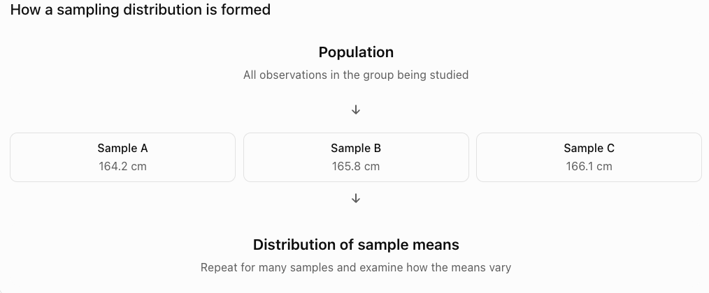
Important Observation
A sampling distribution describes the variation of a statistic, not the variation of individual observations.
This distinction is fundamental to statistical inference.
Three Different Distributions
It is important to distinguish between three related distributions.
Population Distribution
The distribution of all individual observations in the population.
For example, the heights of every student in a school.
Sample Distribution
The distribution of individual observations within one selected sample.
For example, the heights of 30 randomly selected students.
Sampling Distribution
The distribution of a statistic calculated from many possible samples of the same size.
For example, the means of thousands of random samples, each containing 30 students.


Example
Suppose a population has:
Mean = 100
Standard deviation = 20
One sample of 25 observations might have:
Sample mean = 104
Another sample might have:
Sample mean = 97
A third sample might have:
Sample mean = 101
The sampling distribution describes the probabilities associated with these possible sample means.
Sampling Variability
Sampling variability is the natural variation in sample statistics caused by selecting different samples from the same population.
Even when the population does not change, different random samples usually produce different results.
Example
Suppose a school has a population mean mathematics score of 70.
Five random samples of 20 students produce the following means:
68, 72, 69, 71, 70
The sample means vary slightly.
This variation is expected.
Why Does Sampling Variability Occur?
Different samples contain different individuals.
Some samples may include more high-scoring students.
Others may include more low-scoring students.
Consequently, the sample means differ.
Important Observation
Sampling variability does not necessarily indicate a mistake.
It is a normal feature of random sampling.
The Standard Error
The standard error measures the standard deviation of a sampling distribution.
For the sample mean, when observations are independent and drawn from a population with standard deviation σ:
SE(x̄) = σ/√n
where:
-
SE(x̄) = standard error of the sample mean
-
σ = population standard deviation
-
n = sample size
Interpretation
The standard error describes how much sample means typically vary around the population mean.
A smaller standard error means that sample means are more tightly concentrated around the population mean.
A larger standard error means greater sampling variability.
Calculating Standard Error
Suppose a population has:
Mean = 80
Standard deviation = 12
A researcher selects independent random samples of size 36.
Calculate the standard error.
Step 1: Identify the Values
σ = 12
n = 36
Step 2: Apply the Formula
SE(x̄) = 12/√36
SE(x̄) = 12/6
SE(x̄) = 2
Interpretation
The standard deviation of the sampling distribution of sample means is 2.
Although individual observations have a standard deviation of 12, the sample means vary much less.
How Sample Size Affects Sampling Variability
One of the most important properties of sampling distributions is that larger samples generally produce more precise estimates.
For the sample mean:
SE(x̄) = σ/√n
As n increases, the denominator increases.
Therefore, the standard error decreases.
Example
Suppose:
σ = 20
Compare the standard errors for different sample sizes.
|
Sample size |
Standard error |
|---|---|
|
4 |
10 |
|
16 |
5 |
|
25 |
4 |
|
100 |
2 |
|
400 |
1 |
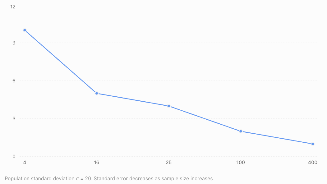
Important Conclusion
Larger samples tend to produce more stable sample means.
However, the improvement follows a square-root relationship.
To reduce the standard error by half, the sample size must be multiplied by four.
Example
If a sample of 25 has a standard error of 4, a sample of 100 will have a standard error of 2, assuming the same population and sampling conditions.
Standard Deviation Versus Standard Error
Standard deviation and standard error measure different types of variability.
|
Standard deviation |
Standard error |
|---|---|
|
Describes variation among individual observations |
Describes variation among sample statistics |
|
Measures spread in a population or sample |
Measures uncertainty due to sampling |
|
Often represented by σ or s |
Often represented by SE |
|
Does not automatically decrease when sample size increases |
Usually decreases as sample size increases |
Example
A population of students has:
Mean height = 165 cm
Standard deviation = 10 cm
A sample of 100 students is selected.
Standard error:
SE = 10/√100
SE = 1 cm
Interpretation
The standard deviation of 10 cm describes differences among individual student heights.
The standard error of 1 cm describes the spread of sample means from repeated samples of 100 students.
These are not interchangeable quantities.
The Central Limit Theorem
The Central Limit Theorem (CLT) is one of the most important ideas in statistics.
It explains why normal distributions frequently appear when analysing sample means.
Statement of the Central Limit Theorem
For independent, identically distributed observations from a population with a finite mean and finite variance, the sampling distribution of the sample mean becomes approximately normal as the sample size increases.
This can occur even when the original population is not normally distributed.
Important Features
-
The original population does not need to be normal.
-
The sample size must be sufficiently large.
-
The population must have a finite mean and variance under the classical version of the theorem.
-
The sampling distribution becomes approximately normal as n increases.
-
The sampling distribution is centred at the population mean.
-
Its standard error is σ/√n for independent observations.

Understanding the Central Limit Theorem
Consider a population with a strongly right-skewed distribution.
Individual observations may be concentrated near low values, with a long tail toward high values.
Now imagine repeatedly selecting random samples and calculating their means.
Small Samples
When the sample size is very small, the distribution of sample means may still be noticeably skewed.
Larger Samples
As the sample size increases, the sampling distribution of the mean generally becomes more symmetric.
Very Large Samples
For sufficiently large samples, the sampling distribution often resembles a normal distribution.
This happens because averaging many independent observations reduces the influence of individual extreme values.
Important Qualification
There is no universal sample size that guarantees a good normal approximation.
The required sample size depends on the shape of the population distribution.
A commonly taught guideline is n ≥ 30, but strongly skewed or heavy-tailed populations may require much larger samples.
When the Population Is Already Normal
If the population itself is normally distributed, the sampling distribution of the sample mean is normal for every positive sample size, assuming independent observations.
Suppose:
X ~ N(μ, σ²)
Then:
x̄ ~ N(μ, σ²/n)
Example
A population has:
Mean = 50
Standard deviation = 10
Independent random samples of size 25 are selected.
The sampling distribution of the sample mean has:
Mean = 50
Standard error = 10/√25 = 2
Therefore:
x̄ ~ N(50, 4)
The second parameter is the variance of the sampling distribution.
Mean of the Sampling Distribution
The mean of the sampling distribution of the sample mean is equal to the population mean.
E(x̄) = μ
This means the sample mean is an unbiased estimator of the population mean under random sampling.
Example
Suppose the population mean is 75.
If we repeatedly select independent random samples and calculate their means, the average of those sample means approaches 75.
Individual samples may produce means above or below 75.
However, the sampling distribution is centred at 75.
Important Observation
Unbiased does not mean every sample estimate is correct.
It means the estimator is correct on average across repeated samples.
Calculating Probabilities Using Sampling Distributions
When the sampling distribution of the mean is normal or approximately normal, we can calculate probabilities using z-scores.
The z-score formula for a sample mean is:
z = (x̄ − μ)/(σ/√n)
This differs from the z-score formula for an individual observation.
For an individual observation:
z = (x − μ)/σ
For a sample mean:
z = (x̄ − μ)/(σ/√n)
The denominator is the standard error rather than the population standard deviation.
Worked Example: Sample Mean Above a Value
A population has:
Mean = 100
Standard deviation = 20
Independent random samples of size 64 are selected.
Assume the sampling distribution is approximately normal.
Find the probability that a sample mean exceeds 105.
Step 1: Calculate the Standard Error
SE = 20/√64
SE = 20/8
SE = 2.5
Step 2: Calculate the z-Score
z = (105 − 100)/2.5
z = 5/2.5
z = 2
Step 3: Find the Probability
P(Z > 2) = 1 − 0.9772
P(Z > 2) ≈ 0.0228
Interpretation
There is approximately a 2.28% probability that a sample of 64 observations will have a mean greater than 105.
This probability describes sample means, not individual observations.
Worked Example: Sample Mean Below a Value
A population has:
Mean = 60
Standard deviation = 12
Independent random samples of size 36 are selected.
Assume the sampling distribution is approximately normal.
Find the probability that a sample mean is below 57.
Step 1: Calculate Standard Error
SE = 12/√36
SE = 2
Step 2: Calculate the z-Score
z = (57 − 60)/2
z = −1.5
Step 3: Find the Probability
P(Z < −1.5) = 0.0668
Final Answer
There is approximately a 6.68% probability that the sample mean is below 57.
Worked Example: Sample Mean Between Two Values
A population has:
Mean = 80
Standard deviation = 15
Independent random samples of size 100 are selected.
Assume the sampling distribution is approximately normal.
Find the probability that the sample mean lies between 77 and 83.
Step 1: Calculate Standard Error
SE = 15/√100
SE = 1.5
Step 2: Calculate the Lower z-Score
z₁ = (77 − 80)/1.5
z₁ = −2
Step 3: Calculate the Upper z-Score
z₂ = (83 − 80)/1.5
z₂ = 2
Step 4: Calculate the Probability
P(−2 ≤ Z ≤ 2) = 0.9772 − 0.0228
P(−2 ≤ Z ≤ 2) ≈ 0.9544
Interpretation
Approximately 95.44% of sample means are expected to fall between 77 and 83.

Sampling Distributions of Proportions
Sampling distributions are not limited to sample means.
They can also describe sample proportions.
Suppose a population contains a proportion p of individuals with a particular characteristic.
A sample is selected, and the proportion possessing that characteristic is calculated.
The sample proportion is represented by:
p̂
Example
Suppose 60% of students at a school prefer online homework.
The population proportion is:
p = 0.60
A random sample of 100 students might produce:
p̂ = 0.57
Another sample might produce:
p̂ = 0.63
These sample proportions vary because of sampling variability.
Mean and Standard Error of a Sample Proportion
Under independent Bernoulli sampling with constant success probability p:
E(p̂) = p
The standard error is:
SE(p̂) = √[p(1 − p)/n]
Worked Example
Suppose:
p = 0.60
n = 100
Calculate the standard error.
Step 1: Substitute
SE(p̂) = √[(0.60 × 0.40)/100]
SE(p̂) = √0.0024
SE(p̂) ≈ 0.049
Interpretation
The sample proportion typically varies around the population proportion by an amount on the order of 0.049, or 4.9 percentage points.
This does not mean every sample proportion will lie within 4.9 percentage points of the true proportion.
Normal Approximation for Sample Proportions
The sampling distribution of a sample proportion can often be approximated by a normal distribution when the sample size is sufficiently large.
A common guideline is:
np ≥ 10
and
n(1 − p) ≥ 10
Example
Suppose:
n = 100
p = 0.60
Then:
np = 60
n(1 − p) = 40
Both values exceed 10.
A normal approximation is generally reasonable under the independence assumptions.
Important Observation
Sample means and sample proportions have different standard-error formulas.
For sample means:
SE(x̄) = σ/√n
For sample proportions:
SE(p̂) = √[p(1 − p)/n]
Sampling With and Without Replacement
Sampling methods can affect the variability of sample statistics.
Sampling With Replacement
After an observation is selected, it is returned to the population before the next selection.
The same observation may be selected more than once.
Under simple random sampling with replacement, draws are independent.
Sampling Without Replacement
After an observation is selected, it is not returned.
The same individual cannot be selected again within that sample.
Draws are dependent because the population changes after each selection.
Why Does This Matter?
When sampling without replacement from a finite population, the standard error may be smaller than the independent-sampling formula suggests.
For a simple random sample without replacement from a finite population, the finite population correction is:
FPC = √[(N − n)/(N − 1)]
The corrected standard error of the sample mean is:
SE(x̄) = (σ/√n) × FPC
This correction is especially relevant when the sample represents a substantial fraction of the population.
For small sampling fractions, the correction is often negligible.
Sampling Error Versus Sampling Bias
Sampling error and sampling bias are different concepts.
Sampling Error
Sampling error is the difference between a sample statistic and the population parameter caused by random selection.
It occurs naturally even when the sampling method is fair.
Sampling Bias
Sampling bias occurs when the selection process systematically favours certain observations.
Example
A school wants to estimate how many students enjoy physical education.
If the researcher surveys only students participating in sports teams, the results may overestimate enthusiasm for physical education.
This is sampling bias.
Important Observation
Increasing sample size reduces random sampling variability.
However, increasing sample size does not automatically eliminate sampling bias.
A very large biased sample can still produce misleading conclusions.
Interpreting Sampling Distribution Graphs
Sampling distributions are commonly represented using histograms or probability curves.
Centre
The centre represents the expected value of the statistic.
For the sample mean:
E(x̄) = μ
Spread
The spread describes sampling variability.
For independent sample means:
SE(x̄) = σ/√n
Shape
The shape depends on the population distribution, sample size, and statistic being examined.
Larger Samples
Larger samples usually produce narrower sampling distributions.
This means the sample statistic is more likely to be close to the population parameter.

Important Interpretation
A narrower sampling distribution indicates greater precision.
It does not necessarily mean the individual observations are less variable.
Real-World Application: Opinion Polling
Opinion polls use samples to estimate the views of larger populations.

Example
A survey estimates that 55% of voters support a proposal.
The sample contains 400 independently selected respondents.
Using the sample proportion as an estimate of p:
p̂ = 0.55
n = 400
Estimated standard error:
SE ≈ √[(0.55 × 0.45)/400]
SE ≈ √0.00061875
SE ≈ 0.0249
Interpretation
The estimated standard error is approximately 2.49 percentage points.
This provides information about random sampling uncertainty.
Other sources of uncertainty, including nonresponse and selection bias, must also be considered.
Real-World Application: Manufacturing Quality Control
Manufacturers use sampling distributions to monitor production processes.

Example
A factory produces components with:
Mean mass = 250 g
Standard deviation = 8 g
A random sample of 64 independent components is selected.
Calculate Standard Error
SE = 8/√64
SE = 8/8
SE = 1 g
Interpretation
The sample mean mass typically varies around the population mean by an amount on the order of 1 g.
A sample mean far from 250 g may indicate an unusual sample or a possible change in the manufacturing process.
However, an unusual sample mean alone does not prove that the process has changed.
Real-World Application: Educational Research
Researchers may use sampling distributions to estimate average examination performance.

Example
A school has 2,000 students.
A researcher selects a random sample of 100 students to estimate average mathematics performance.
The sample mean is 72.
The sample standard deviation is 15.
An estimated standard error is:
SE ≈ 15/√100
SE ≈ 1.5
Interpretation
The estimated standard error describes the sampling variability of the sample mean.
It helps researchers judge the precision of the estimate.
Because the population standard deviation is unknown, the sample standard deviation is used as an estimate.
Real-World Application: Environmental Science
Environmental scientists often estimate population characteristics from samples.

Examples include:
-
Average water temperature.
-
Mean pollutant concentration.
-
Average soil moisture.
-
Proportion of contaminated samples.
-
Average rainfall over a region.
Example
A researcher collects independent water samples from a large lake.
Each sample provides an estimate of the mean pollutant concentration.
Repeated sampling would produce slightly different sample means.
The sampling distribution describes this variation.
Important Consideration
Environmental observations may be correlated across locations or time.
If measurements are not independent, the usual standard-error formula may underestimate uncertainty.
Appropriate sampling designs are therefore important.
Common Mistakes
Confusing a population with a sample
The population is the complete group; the sample is a subset.
Confusing parameters with statistics
Parameters describe populations. Statistics describe samples.
Confusing the sample distribution with the sampling distribution
The sample distribution describes individual observations within one sample.
The sampling distribution describes a statistic across repeated samples.
Assuming every sample gives the same result
Different random samples generally produce different statistics.
Confusing standard deviation with standard error
Standard deviation measures variability among observations.
Standard error measures variability among sample statistics.
Using σ instead of σ/√n for sample-mean probabilities
The sampling distribution of the mean has a smaller spread than the population distribution under independent sampling.
Assuming larger samples eliminate all uncertainty
Larger samples reduce random sampling variability but do not eliminate it.
Assuming the Central Limit Theorem makes the population normal
The theorem concerns the sampling distribution of the mean, not the original population.
Assuming n = 30 always guarantees normality
The required sample size depends on the population distribution.
Ignoring independence assumptions
Dependent observations may require different methods.
Confusing sampling error with sampling bias
Sampling error arises from random variation; bias arises from systematic problems in selection or measurement.
Assuming an unbiased estimator is always accurate
Unbiased means correct on average, not correct in every sample.
Key Terms
-
Population: Complete group of individuals or observations being studied.
-
Sample: Subset of a population.
-
Population Parameter: Numerical characteristic of a population.
-
Sample Statistic: Numerical characteristic calculated from a sample.
-
Population Mean (μ): Average of all population observations.
-
Sample Mean (x̄): Average of observations within a sample.
-
Population Standard Deviation (σ): Measure of population variability.
-
Sample Standard Deviation (s): Measure of variability within a sample.
-
Sampling Distribution: Probability distribution of a statistic across possible samples.
-
Sampling Variability: Natural variation in sample statistics caused by random sampling.
-
Sampling Error: Difference between a sample statistic and its population parameter.
-
Standard Error: Standard deviation of a sampling distribution.
-
Central Limit Theorem: Theorem describing the approximate normality of sample means for sufficiently large independent samples under suitable conditions.
-
Unbiased Estimator: Estimator whose expected value equals the parameter being estimated.
-
Sample Size
-
Population Size (N): Number of observations in the population.
-
Random Sampling: Sampling process involving random selection.
-
Sampling With Replacement: Method in which selected observations are returned before subsequent selections.
-
Sampling Without Replacement: Method in which selected observations are not returned.
-
Finite Population Correction: Adjustment for sampling without replacement from a finite population.
-
Sample Proportion (p̂): Proportion of sample observations with a particular characteristic.
-
Population Proportion (p): Proportion of the population with a particular characteristic.
-
Normal Approximation: Use of a normal distribution to approximate another distribution.
-
Sampling Bias: Systematic distortion caused by the sampling process.
-
Statistical Inference: Use of sample information to draw conclusions about populations.
-
Precision: Degree to which repeated estimates are concentrated around one another.
Key Takeaways
-
Sampling distributions describe how sample statistics vary across repeated samples.
-
A population parameter is fixed, while a sample statistic varies from sample to sample.
-
Sampling variability occurs naturally because different samples contain different observations.
-
The sampling distribution of the sample mean is centred at the population mean.
-
The standard error measures the spread of the sampling distribution.
-
For independent observations, SE(x̄) = σ/√n.
-
Larger samples generally produce smaller standard errors.
-
To halve the standard error, the sample size must be multiplied by four.
-
The Central Limit Theorem explains why sample means often follow approximately normal distributions for sufficiently large samples.
-
The original population does not need to be normally distributed.
-
A normal population produces normally distributed sample means for any sample size under independent sampling.
-
Sample means and sample proportions have different standard-error formulas.
-
Sampling error is different from sampling bias.
-
Larger samples reduce random sampling variability but do not automatically correct biased sampling.
-
Sampling distributions are fundamental to statistical inference, confidence intervals, and hypothesis testing.
Check Your Understanding
Populations and Samples
-
Define a population.
-
Define a sample.
-
Explain the difference between a parameter and a statistic.
-
What symbol represents the population mean?
-
What symbol represents the sample mean?
Sampling Distributions
-
Define a sampling distribution.
-
Explain why sample means vary between samples.
-
What is sampling variability?
-
What is the mean of the sampling distribution of the sample mean?
-
Explain the difference between standard deviation and standard error.
Central Limit Theorem
-
State the Central Limit Theorem in your own words.
-
Does the original population need to be normal?
-
What generally happens to the sampling distribution as sample size increases?
-
Why is n = 30 not a universal guarantee of normality?
-
Explain why the Central Limit Theorem is important in statistics.
Calculations
-
Calculate the standard error when σ = 20 and n = 25.
-
Calculate the standard error when σ = 15 and n = 100.
-
A population has mean 80, standard deviation 12, and sample size 36. Calculate the z-score for a sample mean of 84.
-
A population proportion is 0.40 and n = 100. Calculate the standard error of the sample proportion.
-
Explain what happens to standard error when sample size is multiplied by four.
Answer Key
|
Question |
Answer |
|---|---|
|
1 |
Complete group being studied |
|
2 |
Subset of a population |
|
3 |
Parameters describe populations; statistics describe samples |
|
4 |
μ |
|
5 |
x̄ |
|
6 |
Distribution of a statistic across possible samples |
|
7 |
Different samples contain different observations |
|
8 |
Natural variation in sample statistics |
|
9 |
μ |
|
10 |
Standard deviation describes observations; standard error describes sample statistics |
|
11 |
Sample means become approximately normal for sufficiently large samples under suitable conditions |
|
12 |
No |
|
13 |
It becomes narrower and often more nearly normal |
|
14 |
Required sample size depends on population shape |
|
15 |
It allows normal probability methods to be applied to many sample means |
|
16 |
4 |
|
17 |
1.5 |
|
18 |
2 |
|
19 |
Approximately 0.049 |
|
20 |
It is halved |
Extended Challenge
Understanding Sampling Distributions
-
Explain why the sampling distribution of the mean is different from the population distribution.
-
Describe how repeated random sampling can be used to construct a sampling distribution.
-
Explain why the sample mean is an unbiased estimator of the population mean.
-
Describe the effect of increasing sample size on sampling variability.
-
Explain why a larger sample does not necessarily eliminate sampling bias.
Standard Error Calculations
-
Calculate the standard error for σ = 24 and n = 36.
-
Calculate the standard error for σ = 18 and n = 81.
-
Calculate the sample size required to reduce a standard error of 6 to 3.
-
A population has standard deviation 30. Find the sample size required for a standard error of 3.
-
Explain why standard error decreases according to a square-root relationship.
Central Limit Theorem
-
Explain why sample means can be approximately normal even when the population is skewed.
-
Describe a situation where the Central Limit Theorem might require a very large sample.
-
Explain why the sampling distribution of a normal population is normal for every sample size.
-
Discuss the importance of independence in the Central Limit Theorem.
-
Explain why the theorem is useful for calculating probabilities.
Practical Applications
-
A population has mean 100 and standard deviation 20. Independent samples of size 100 are selected. Find P(x̄ > 104), assuming an approximately normal sampling distribution.
-
A population has mean 60 and standard deviation 15. Independent samples of size 25 are selected. Find P(x̄ < 57), assuming an approximately normal sampling distribution.
-
A population proportion is 0.30. Find the standard error for n = 400 under independent Bernoulli sampling.
-
Explain how sampling distributions help researchers estimate population characteristics.
-
Describe how sampling bias can affect conclusions even when the standard error is small.
Final Investigation: Estimating Student Examination Performance
A school has 2,500 students.
The population mean mathematics score is 70.
The population standard deviation is 15.
Researchers investigate the sampling distribution of the mean using independent random samples.
Investigation Tasks
-
Identify the population.
-
Identify the population mean.
-
Identify the population standard deviation.
-
Explain what a sample mean represents.
-
Define the sampling distribution of the sample mean.
-
Calculate the standard error for n = 25.
-
Calculate the standard error for n = 100.
-
Calculate the standard error for n = 225.
-
Compare the three standard errors.
-
Explain why larger samples produce smaller standard errors.
-
Sketch the sampling distributions for the three sample sizes on the same scale.
-
Identify which distribution is narrowest.
-
Explain why all three distributions have the same centre.
-
Calculate the z-score for x̄ = 73 when n = 100.
-
Find P(x̄ > 73) for n = 100, assuming an approximately normal sampling distribution.
-
Calculate the probability that x̄ lies between 67 and 73 when n = 100.
-
Explain how the Central Limit Theorem supports the probability calculations.
-
Discuss why a biased sample might produce misleading results.
-
Explain how the researchers could improve the sampling procedure.
-
Write a statistical report describing the relationship between sample size, standard error, and the reliability of sample estimates.
5. Applications of Probability Distributions
Learning outcomes
- I can select appropriate probability models.
- I can solve real-world probability problems.
- I can interpret statistical results.
- I can evaluate statistical models.
- I can communicate conclusions clearly.
Applications of Probability Distributions
Introduction
Probability distributions are mathematical models used to describe uncertainty and predict the likelihood of different outcomes.
They are used in many areas of everyday life, including business, medicine, engineering, environmental science, education, sports, and economics.
For example:
-
A manufacturer may want to estimate the probability that a product is defective.
-
A hospital may need to predict how many patients will arrive during an hour.
-
A teacher may want to analyse examination results.
-
A meteorologist may estimate the probability of extreme rainfall.
-
A business may need to predict future sales.
-
An insurance company may calculate the expected cost of claims.
Different situations require different probability models.
Choosing the correct distribution is essential because an inappropriate model can produce misleading conclusions, even when the calculations are mathematically correct.


Why Are Probability Distributions Useful?
A probability distribution describes the possible values of a random variable and the likelihood of those values occurring.
Probability distributions allow us to:
-
Estimate the likelihood of particular events.
-
Predict expected outcomes.
-
Measure uncertainty and variability.
-
Compare different decisions.
-
Identify unusual observations.
-
Evaluate risks.
-
Make decisions using statistical evidence.
Example
A factory knows that approximately 4% of its products are defective.
Rather than inspecting every product, the factory may use a probability model to estimate the likelihood of finding defective items in a sample.
This information can help determine inspection procedures and quality-control standards.
Important Observation
Probability models do not guarantee particular outcomes.
They describe uncertainty and the likelihood of different possibilities.
Choosing an Appropriate Probability Model
The first step in solving a probability problem is identifying the type of random variable and the structure of the experiment.
Discrete Random Variables
Discrete random variables take countable values.
Examples include:
-
Number of defective products.
-
Number of successful attempts.
-
Number of customers arriving.
-
Number of telephone calls received.
Continuous Random Variables
Continuous random variables take values across numerical intervals.
Examples include:
-
Height.
-
Mass.
-
Temperature.
-
Time.
-
Distance.
-
Measurement error.
Common Probability Models
|
Model |
Type |
Typical application |
|---|---|---|
|
Bernoulli |
Discrete |
One success-or-failure trial |
|
Binomial |
Discrete |
Number of successes in a fixed number of independent trials |
|
Geometric |
Discrete |
Number of trials until the first success |
|
Poisson |
Discrete |
Number of events in a fixed interval |
|
Discrete uniform |
Discrete |
Equally likely numerical outcomes |
|
Continuous uniform |
Continuous |
Equally likely values across an interval |
|
Normal |
Continuous |
Approximately symmetric, bell-shaped measurements |
|
Exponential |
Continuous |
Waiting time between events in a Poisson process |
These distributions have different assumptions and mathematical properties.
A Guide to Selecting Probability Models
Probability model selection
What type of outcome are you studying?
Discrete
One success/failure trial
Bernoulli
Successes in fixed independent trials
Binomial
Trials until first success
Geometric
Event counts over an interval
Poisson
Continuous
Constant density over an interval
Uniform
Symmetric bell-shaped measurements
Normal
Waiting time in a Poisson process
Exponential
Important Questions
Before selecting a probability distribution, ask:
-
Is the variable discrete or continuous?
-
Are we counting events or measuring a quantity?
-
Is the number of trials fixed?
-
Are trials independent?
-
Does the probability of success remain constant?
-
Are events occurring at a constant average rate?
-
Is the observed distribution approximately symmetric?
-
Does the model reflect the real-world situation?
Bernoulli Distribution
A Bernoulli distribution describes a single experiment with two possible outcomes.
These outcomes are usually called success and failure.
Let:
X = 1 for success
X = 0 for failure
If the probability of success is p:
P(X = 1) = p
P(X = 0) = 1 − p
Example
A product has a 3% probability of being defective.
Let X = 1 if the product is defective and X = 0 otherwise.
Then:
P(X = 1) = 0.03
P(X = 0) = 0.97
Expected Value
E(X) = p
Variance
Var(X) = p(1 − p)
When Is This Model Appropriate?
Use a Bernoulli distribution when studying one trial with two possible outcomes.
Binomial Distribution
A binomial distribution describes the number of successes in a fixed number of independent trials with constant success probability.
Conditions
-
Fixed number of trials.
-
Two possible outcomes per trial.
-
Independent trials.
-
Constant probability of success.
Formula
P(X = k) = C(n, k)pᵏ(1 − p)ⁿ⁻ᵏ
where:
-
n = number of trials
-
k = number of successes
-
p = probability of success
-
C(n, k) = number of combinations
Expected Value
E(X) = np
Variance
Var(X) = np(1 − p)
Worked Example: Defective Products
A factory produces electronic components.
Each component has a 5% probability of being defective.
Ten independently produced components are inspected.
Find the probability that exactly two are defective.
Step 1: Identify the Distribution
X ~ Bin(10, 0.05)
n = 10
p = 0.05
k = 2
Step 2: Apply the Formula
P(X = 2) = C(10, 2)(0.05)²(0.95)⁸
C(10, 2) = 45
P(X = 2) = 45 × 0.0025 × 0.66342
P(X = 2) ≈ 0.0746
Interpretation
There is approximately a 7.46% probability that exactly two of the ten components will be defective.

Geometric Distribution
A geometric distribution models the number of independent trials required to obtain the first success when each trial has the same probability of success.
Example
A basketball player has a 70% probability of making each free throw.
Let X represent the number of attempts required to make the first successful shot.
Possible values:
X = 1, 2, 3, 4, ...
Formula
P(X = k) = (1 − p)ᵏ⁻¹p
where:
-
p = probability of success
-
k = trial number of the first success
Worked Example
Find the probability that the player makes the first successful shot on the third attempt.
p = 0.70
k = 3
P(X = 3) = (0.30)²(0.70)
P(X = 3) = 0.09 × 0.70
P(X = 3) = 0.063
Interpretation
There is a 6.3% probability that the player's first successful shot occurs on the third attempt.
Expected Value
For this definition of the geometric random variable:
E(X) = 1/p
For p = 0.70:
E(X) = 1/0.70
E(X) ≈ 1.43 attempts
Poisson Distribution
The Poisson distribution models the number of events occurring in a fixed interval of time, distance, area, or another exposure measure.
It is useful when events occur independently at a constant average rate.
Examples include:
-
Telephone calls received per minute.
-
Customers arriving at a service desk.
-
Radioactive decay events.
-
Defects per metre of material.
-
Equipment failures over time.
Poisson Formula
P(X = k) = e⁻λ λᵏ/k!
where:
-
λ = expected number of events in the interval
-
k = number of events
-
e ≈ 2.71828
Expected Value
E(X) = λ
Variance
Var(X) = λ
Worked Example: Customer Arrivals
A shop receives an average of four customers every ten minutes.
Assume customer arrivals follow a Poisson process.
Find the probability that exactly three customers arrive during a ten-minute interval.
Step 1: Identify the Values
λ = 4
k = 3
Step 2: Apply the Formula
P(X = 3) = e⁻⁴ × 4³/3!
P(X = 3) = e⁻⁴ × 64/6
P(X = 3) ≈ 0.0183156 × 10.6667
P(X = 3) ≈ 0.1954
Interpretation
There is approximately a 19.54% probability that exactly three customers arrive during a ten-minute interval.

Uniform Distribution
A uniform distribution describes situations where outcomes have equal probabilities or equal probability density.
There are two main forms.
Discrete Uniform Distribution
A discrete uniform distribution has a finite number of equally likely outcomes.
Example
Rolling a fair six-sided die.
Each value has probability:
P(X = x) = 1/6
The expected value is:
E(X) = (1 + 2 + 3 + 4 + 5 + 6)/6
E(X) = 3.5
Continuous Uniform Distribution
A continuous uniform distribution has constant probability density over an interval.
For X uniformly distributed between a and b:
f(x) = 1/(b − a)
for a ≤ x ≤ b.
Probability Formula
P(c ≤ X ≤ d) = (d − c)/(b − a)
provided a ≤ c ≤ d ≤ b.
Expected Value
E(X) = (a + b)/2
Worked Example: Waiting Time
A bus arrives at a random time during a 20-minute interval.
Assume every arrival time within the interval is equally likely.
Find the probability that a passenger waits between 5 and 12 minutes.
Step 1: Identify the Interval
Total interval = 20 minutes
Desired interval = 12 − 5 = 7 minutes
Step 2: Calculate the Probability
P(5 ≤ X ≤ 12) = 7/20
P(5 ≤ X ≤ 12) = 0.35
Interpretation
There is a 35% probability that the waiting time is between 5 and 12 minutes.

Normal Distribution
The normal distribution is a continuous probability distribution that is symmetric and bell-shaped.
It is commonly used to model:
-
Measurement errors.
-
Some biological measurements.
-
Some examination results.
-
Manufacturing measurements.
-
Averages of large samples.
Characteristics
-
Symmetric around the mean.
-
Mean, median, and mode are equal.
-
Total area under the curve is 1.
-
Shape determined by mean and standard deviation.
Normal Distribution Notation
X ~ N(μ, σ²)
z-Score Formula
z = (x − μ)/σ
Worked Example: Examination Scores
Examination scores are approximately normally distributed with:
Mean = 70
Standard deviation = 10
Find the probability that a randomly selected student scores above 85.
Step 1: Calculate the z-Score
z = (85 − 70)/10
z = 1.5
Step 2: Find the Probability
P(Z ≤ 1.5) = 0.9332
P(Z > 1.5) = 1 − 0.9332
P(Z > 1.5) = 0.0668
Interpretation
Approximately 6.68% of students are expected to score above 85 under the normal model.

Exponential Distribution
The exponential distribution models the waiting time between events in a Poisson process.
Examples include:
-
Time between customer arrivals.
-
Time between certain equipment failures.
-
Time between radioactive decay events.
-
Time between calls received by a service centre.
Probability Formula
For a waiting time X with rate λ:
P(X > t) = e⁻λᵗ
where:
-
λ = average event rate per unit time
-
t = waiting time
Expected Value
E(X) = 1/λ
Worked Example
A service centre receives an average of three calls per hour.
Assume calls arrive according to a Poisson process.
Find the probability that the waiting time until the next call exceeds 20 minutes.
Step 1: Convert Time
20 minutes = 1/3 hour
Step 2: Identify the Rate
λ = 3 calls per hour
Step 3: Apply the Formula
P(X > 1/3) = e⁻³⁽¹/³⁾
P(X > 1/3) = e⁻¹
P(X > 1/3) ≈ 0.3679
Interpretation
There is approximately a 36.79% probability that the next call will arrive more than 20 minutes later.
Comparing Probability Distributions
|
Distribution |
Main question |
Important parameter |
|---|---|---|
|
Bernoulli |
Does one trial succeed? |
p |
|
Binomial |
How many successes in n trials? |
n, p |
|
Geometric |
How many trials until first success? |
p |
|
Poisson |
How many events occur in an interval? |
λ |
|
Discrete uniform |
Which equally likely numerical outcome occurs? |
Number of outcomes |
|
Continuous uniform |
Where does a value fall in an interval? |
a, b |
|
Normal |
How far is a measurement from the mean? |
μ, σ |
|
Exponential |
How long until the next event? |
λ |
Important Observation
Two models may describe different aspects of the same process.
For example, a Poisson distribution can describe the number of calls arriving during an hour.
An exponential distribution can describe the waiting time until the next call.
The appropriate model depends on the question being asked.
Solving Real-World Probability Problems
A reliable method for solving probability problems involves six steps.
Identify the Random Variable
Define exactly what is being measured or counted.
For example:
X = number of defective products.
Select the Distribution
Determine which probability model best describes the situation.
Check the Assumptions
Confirm that the conditions of the model are reasonable.
Identify the Parameters
Determine the necessary values, such as:
n, p, λ, μ, or σ.
Calculate the Probability
Apply the appropriate formula or statistical method.
Interpret the Result
Explain what the numerical answer means in the context of the original problem.
Example
A factory has a defect rate of 2%.
Twenty independently produced products are selected.
Find the probability that at least one product is defective.
Step 1: Define the Variable
X = number of defective products.
Step 2: Select the Model
Binomial distribution.
Step 3: Identify the Parameters
n = 20
p = 0.02
Step 4: Use the Complement Rule
P(X ≥ 1) = 1 − P(X = 0)
P(X ≥ 1) = 1 − (0.98)²⁰
P(X ≥ 1) ≈ 1 − 0.6676
P(X ≥ 1) ≈ 0.3324
Interpretation
There is approximately a 33.24% probability that at least one of the twenty products will be defective.
Expected Value in Decision-Making
Expected value is useful when comparing decisions involving uncertainty.
For a discrete random variable:
E(X) = Σ[x × P(X = x)]
Worked Example: Business Investment
A business considers investing in a new product.
The possible profits are:
|
Outcome |
Profit |
Probability |
|---|---|---|
|
High demand |
$20,000 |
0.30 |
|
Moderate demand |
$8,000 |
0.50 |
|
Low demand |
−$5,000 |
0.20 |
Step 1: Calculate Weighted Outcomes
High demand:
20,000 × 0.30 = 6,000
Moderate demand:
8,000 × 0.50 = 4,000
Low demand:
−5,000 × 0.20 = −1,000
Step 2: Add
E(X) = 6,000 + 4,000 − 1,000
E(X) = $9,000
Interpretation
The expected profit is $9,000.
This does not guarantee a profit of $9,000.
The actual outcome may be a large profit, a moderate profit, or a loss.
Important Consideration
Expected value is not the only factor in decision-making.
Businesses may also consider:
-
Financial risk.
-
Available resources.
-
Worst-case outcomes.
-
Variability of returns.
-
Long-term consequences.
Interpreting Statistical Results
A probability calculation is only useful when its meaning is correctly explained.
Probability Versus Certainty
A probability of 0.80 does not guarantee that an event will occur.
It means the event has an 80% probability under the model.
Expected Value Versus Actual Outcome
An expected value of 3.5 successes does not mean that 3.5 successes will occur in an individual experiment.
It represents a long-run average.
Statistical Models Versus Reality
Models simplify real-world situations.
A model may assume independence or constant probabilities even when real-world conditions are more complicated.
Example
A basketball player may have a historical free-throw success rate of 80%.
However, performance may change due to:
-
Fatigue.
-
Injury.
-
Pressure.
-
Training.
-
Environmental conditions.
A binomial model may be useful, but its assumptions should be evaluated.
Evaluating Statistical Models
A statistical model should be assessed before its conclusions are accepted.
Accuracy
Does the model produce predictions that are reasonably consistent with observed data?
Assumptions
Are the assumptions realistic?
For example, are repeated trials truly independent?
Data Quality
Were the data collected using a reliable method?
Sample Size
Is there enough information to estimate model parameters reliably?
Outliers
Are unusual observations affecting the results?
Model Limitations
Does the model ignore important real-world factors?
Example: Customer Arrivals
A Poisson model assumes events occur independently at a constant average rate.
However, customer arrivals may be more frequent during lunchtime and less frequent during the evening.
A single constant-rate Poisson model may not describe the entire day accurately.
A better model might use different arrival rates for different time periods.
Comparing Model Predictions with Observed Data
One way to evaluate a model is to compare its predicted probabilities with observed frequencies.
Example
A factory predicts that 5% of products are defective.
During an inspection, 1,000 products are examined.
The expected number of defective products is:
E(X) = 1,000 × 0.05
E(X) = 50
Suppose the inspector finds 83 defective products.
Interpretation
The observed number is substantially higher than the expected value.
This may suggest that:
-
The defect rate has increased.
-
The original estimate was inaccurate.
-
The sample was unusual.
-
The independence or constant-probability assumptions are inappropriate.
Important Observation
A difference between observed and expected values does not automatically prove that the model is wrong.
Random variation must also be considered.
Formal statistical tests can help determine whether the difference is unusually large under the model.
Using Graphs to Evaluate Probability Models
Graphs can reveal whether a theoretical distribution matches observed data.
Histograms
Histograms show the shape of numerical data.
They can reveal:
-
Symmetry.
-
Skewness.
-
Multiple peaks.
-
Gaps.
-
Outliers.
Probability Distribution Graphs
These show the theoretical probabilities assigned to possible outcomes.
Box Plots
Box plots summarise the median, quartiles, and spread of data.
Normal Probability Plots
Normal probability plots help assess whether data are reasonably consistent with a normal distribution.


Important Observation
A graph may suggest that a model is inappropriate, but visual inspection alone may not provide a complete evaluation.
Numerical summaries and statistical tests may also be useful.
Understanding Risk and Uncertainty
Probability models help quantify risk.
Risk involves the possibility of an undesirable outcome and its potential consequences.
Example
Consider two investments.
Investment A:
-
Expected profit = $5,000.
-
Small variability.
Investment B:
-
Expected profit = $7,000.
-
Large variability.
Investment B has a higher expected profit.
However, it may also have a greater probability of a substantial loss.
Important Observation
A higher expected value does not always make an option preferable.
Decision-makers must consider both expected outcomes and uncertainty.
Communicating Statistical Conclusions
Statistical conclusions should be clear, accurate, and connected to the original question.
A strong statistical conclusion should include:
-
The probability model used.
-
The relevant assumptions.
-
The calculated result.
-
An explanation of the result in context.
-
Any important limitations.
Weak Conclusion
"The probability is 0.067."
This statement provides a number but little meaning.
Strong Conclusion
"Using a normal distribution with a mean of 70 and standard deviation of 10, the probability that a student scores above 85 is approximately 6.7%. This estimate assumes the examination scores are reasonably described by the normal model."
The stronger conclusion identifies the model, explains the result, and acknowledges an assumption.
Avoid Overstating Conclusions
Statistical results describe uncertainty.
Avoid statements such as:
-
"This event will definitely happen."
-
"The model proves the outcome."
-
"Every sample will have the expected value."
Instead, use language such as:
-
"The model predicts..."
-
"The probability is approximately..."
-
"The expected value is..."
-
"The evidence suggests..."
-
"Under the stated assumptions..."
Real-World Application: Healthcare
Healthcare researchers use probability distributions to model patient outcomes and service demand.

Example
A hospital estimates that 10% of patients require an additional follow-up appointment.
Suppose 50 independent patients are selected, each with the same probability.
Let X represent the number requiring follow-up.
X ~ Bin(50, 0.10)
Expected Value
E(X) = 50 × 0.10
E(X) = 5
Interpretation
The hospital expects approximately five patients in the group to require follow-up.
This estimate may help with staffing and appointment planning.
However, actual patient needs may vary.
Real-World Application: Environmental Science
Environmental scientists use probability models to study rainfall, pollution, temperature, and extreme events.

Example
Suppose the number of heavy rainfall events in a region follows a Poisson distribution with an average of two events per month.
Find the probability of no heavy rainfall events during a month.
Step 1: Identify the Values
λ = 2
k = 0
Step 2: Apply the Formula
P(X = 0) = e⁻² × 2⁰/0!
P(X = 0) = e⁻²
P(X = 0) ≈ 0.1353
Interpretation
There is approximately a 13.53% probability of no heavy rainfall events during a month under the Poisson model.
Actual weather patterns may violate the assumptions of a constant-rate process.
Real-World Application: Engineering
Engineers use probability models to study manufacturing tolerances, measurement errors, and equipment reliability.

Example
A machine produces metal rods with lengths approximately normally distributed.
Mean = 100 mm
Standard deviation = 0.5 mm
Find the probability that a rod has a length between 99 mm and 101 mm.
Step 1: Calculate z-Scores
Lower boundary:
z = (99 − 100)/0.5 = −2
Upper boundary:
z = (101 − 100)/0.5 = 2
Step 2: Calculate Probability
P(−2 ≤ Z ≤ 2) ≈ 0.9544
Interpretation
Approximately 95.44% of rods are expected to fall within the specified length interval.
This information can help engineers evaluate manufacturing consistency.
Common Mistakes
Choosing a distribution without checking its assumptions
A familiar formula is not necessarily the correct model.
Confusing discrete and continuous variables
Counts are generally discrete, while measurements are often continuous.
Using a binomial model when trials are dependent
Dependence can invalidate the standard binomial assumptions.
Using a Poisson model without considering the event rate
A changing event rate may require a different model.
Assuming every measurement is normally distributed
Real-world measurements may be skewed or multimodal.
Confusing expected value with the most likely outcome
The expected value and mode are not necessarily equal.
Confusing probability with certainty
A high probability does not guarantee an outcome.
Ignoring units
Probabilities are unitless, but expected values and standard deviations retain the units of the random variable.
Using the wrong parameter
Different distributions require different parameters.
Ignoring model limitations
Every statistical model simplifies reality.
Overinterpreting unusual observations
An unusual result does not automatically prove that a model is incorrect.
Communicating only a numerical answer
A useful conclusion explains the meaning of the result in context.
Key Terms
-
Probability Distribution: Mathematical description of possible outcomes and their probabilities.
-
Probability Model: Mathematical representation of uncertainty.
-
Random Variable: Numerical value assigned to outcomes of a random experiment.
-
Discrete Random Variable: Random variable with countable possible values.
-
Continuous Random Variable: Random variable taking values across continuous intervals.
-
Bernoulli Distribution: Distribution describing one success-or-failure trial.
-
Binomial Distribution: Distribution describing successes in a fixed number of independent trials.
-
Geometric Distribution: Distribution describing the number of trials until the first success.
-
Poisson Distribution: Distribution describing event counts in fixed intervals under suitable assumptions.
-
Uniform Distribution: Distribution with equally likely outcomes or constant density.
-
Normal Distribution: Continuous symmetric bell-shaped probability distribution.
-
Exponential Distribution: Distribution describing waiting times in a Poisson process.
-
Expected Value: Probability-weighted average of a random variable.
-
Variance: Measure of the spread of a probability distribution.
-
Standard Deviation: Square root of variance.
-
Parameter: Numerical value describing a probability model or population.
-
Probability Density: Function describing probability per unit interval for continuous variables.
-
Cumulative Probability: Probability of an outcome at or below a specified value.
-
Independence: Condition where one event does not affect another's probability.
-
Assumption: Condition required for a model or calculation to be appropriate.
-
Model Accuracy: Degree to which a model agrees with observed data.
-
Model Validation: Process of evaluating whether a model describes data adequately.
-
Sampling Variability: Natural variation arising from random sampling.
-
Statistical Inference: Use of sample evidence to draw conclusions about a population.
-
Risk: Possibility and consequences of an undesirable outcome.
-
Uncertainty: Lack of certainty about future or unknown outcomes.
Key Takeaways
-
Probability distributions help describe uncertainty and predict outcomes.
-
Different situations require different probability models.
-
The type of random variable helps determine which distribution may be appropriate.
-
Bernoulli distributions describe single binary trials.
-
Binomial distributions describe numbers of successes in fixed independent trials.
-
Geometric distributions describe trials until the first success.
-
Poisson distributions describe event counts over intervals.
-
Uniform distributions describe equally likely outcomes or constant density.
-
Normal distributions describe approximately symmetric bell-shaped measurements.
-
Exponential distributions describe waiting times in Poisson processes.
-
Expected value describes the long-run average outcome.
-
Variance and standard deviation describe variability.
-
Model assumptions must be checked before calculations are interpreted.
-
Observed data should be compared with model predictions.
-
Statistical conclusions should include context, assumptions, and limitations.
-
Probability models support decision-making but do not guarantee outcomes.
Check Your Understanding
Selecting Probability Models
-
Which distribution describes a single success-or-failure trial?
-
Which distribution models the number of successes in ten independent trials?
-
Which distribution models the number of trials until the first success?
-
Which distribution may model customer arrivals during an hour?
-
Which distribution is commonly used for symmetric bell-shaped measurements?
Solving Probability Problems
-
A fair coin is tossed five times. Which distribution is appropriate for the number of heads?
-
A fair die is rolled once. Which distribution describes the equally likely numerical outcomes?
-
A shop receives an average of three customers per minute. Which distribution may model the number arriving in one minute?
-
A bus arrives uniformly during a 15-minute interval. What is the probability of waiting less than five minutes?
-
A product has a 10% defect probability. What is the expected number of defective products in 50 independent items?
Interpreting Results
-
What does an expected value represent?
-
Why does a probability of 0.90 not guarantee an event?
-
Explain why model assumptions are important.
-
What is the difference between a model prediction and an observed result?
-
Why might a statistical model become less accurate over time?
Evaluating Models
-
Why might a binomial model be inappropriate for dependent trials?
-
Why might a Poisson model be inappropriate when arrival rates change throughout the day?
-
Explain why a normal model may be inappropriate for strongly skewed data.
-
Describe one method for comparing a model with observed data.
-
Identify two features of a clear statistical conclusion.
Answer Key
|
Question |
Answer |
|---|---|
|
1 |
Bernoulli |
|
2 |
Binomial |
|
3 |
Geometric |
|
4 |
Poisson |
|
5 |
Normal |
|
6 |
Binomial |
|
7 |
Discrete uniform |
|
8 |
Poisson, if its assumptions hold |
|
9 |
5/15 = 1/3 |
|
10 |
5 |
|
11 |
Long-run probability-weighted average |
|
12 |
The event can still fail to occur |
|
13 |
They determine whether the model is appropriate |
|
14 |
Prediction is theoretical; observation is measured |
|
15 |
Conditions and probabilities may change |
|
16 |
Independence is required |
|
17 |
A constant rate is assumed |
|
18 |
Normal distributions are symmetric |
|
19 |
Compare observed frequencies with predicted probabilities |
|
20 |
Contextual interpretation and acknowledgement of assumptions or limitations |
Extended Challenge
Selecting Appropriate Models
-
A factory inspects twenty independently produced products and counts defects. Identify the appropriate distribution.
-
A researcher measures the heights of 500 adults. Explain when a normal model may be appropriate.
-
A shop counts customer arrivals during ten-minute intervals. Explain when a Poisson model may be appropriate.
-
A player rolls a die until the first six appears. Identify the distribution.
-
A passenger waits for a bus that arrives uniformly during a 30-minute interval. Identify the distribution.
Probability Calculations
-
A fair coin is tossed six times. Find the probability of exactly three heads.
-
A product has a 4% defect rate. Find the probability of no defects in ten independent products.
-
A shop receives an average of five customers per hour according to a Poisson process. Find the probability of exactly three arrivals in an hour.
-
A normal distribution has mean 100 and standard deviation 15. Find the probability of an observation exceeding 130.
-
A waiting time is uniformly distributed between 0 and 20 minutes. Find the probability of waiting between 8 and 15 minutes.
Expected Value and Risk
-
A game awards $20 with probability 0.2 and nothing otherwise. Calculate the expected prize.
-
If the game costs $5, calculate the expected net gain.
-
Explain why a higher expected profit does not always indicate a better investment.
-
Describe how variance can help compare two risky decisions.
-
Explain why businesses use probability models when planning inventory.
Model Evaluation
-
A factory predicts 2% defective products but observes 8% in a large sample. Explain possible reasons for the difference.
-
Explain how a histogram can help evaluate a normal model.
-
Describe a situation where a model's independence assumption might fail.
-
Explain why a model should be updated when new data become available.
-
Write a short statistical conclusion that includes a calculated probability, its meaning, and a limitation.
Final Investigation: Choosing the Best Probability Model
A research team investigates four different situations.
Situation A: Manufacturing
A factory produces electronic components.
Each component has a 3% probability of being defective.
Twenty independently produced components are inspected.
Situation B: Customer Arrivals
A shop receives an average of six customers per hour.
Assume arrivals follow a Poisson process.
Situation C: Examination Results
Examination scores are approximately normally distributed.
Mean = 70
Standard deviation = 12
Situation D: Waiting Time
A bus arrives uniformly at random during a 20-minute interval.
Investigation Tasks
-
Identify the random variable in Situation A.
-
Select the appropriate probability distribution for Situation A.
-
Explain why the distribution is appropriate.
-
Calculate the probability of exactly one defective component.
-
Calculate the expected number of defective components.
-
Identify the random variable in Situation B.
-
Select the appropriate distribution for Situation B.
-
Calculate the probability of exactly four customers arriving in one hour.
-
Calculate the probability of no customers arriving in one hour.
-
Explain one limitation of the model in Situation B.
-
Identify the distribution used in Situation C.
-
Calculate the z-score for an examination score of 88.
-
Calculate the probability of scoring above 88.
-
Calculate the probability of scoring between 58 and 82.
-
Explain how the results could help a teacher interpret student performance.
-
Identify the distribution used in Situation D.
-
Calculate the probability of waiting less than five minutes.
-
Calculate the probability of waiting between 8 and 15 minutes.
-
Compare the assumptions and limitations of all four models.
-
Write a statistical report explaining how probability distributions support real-world decision-making.