Modelling Real-World Situations with Quadratic Functions

Introduction

Mathematics helps us describe, understand, and predict events in the real world. One particularly useful type of mathematical relationship is a quadratic function.

Quadratic functions are used to model situations involving curved paths, maximum and minimum values, changing areas, profits, costs, and many other relationships.

For example:

• The height of a ball thrown into the air changes over time.

• The area of a rectangular garden depends on its dimensions.

• The profit earned by a business may increase and then decrease as production changes.

• The braking distance of a vehicle increases approximately with the square of its speed under suitable conditions.

• The shape of a parabolic arch can be described using a quadratic equation.

A quadratic model allows us to represent these situations mathematically and use equations, graphs, and tables to make predictions.

However, not every real-world relationship is quadratic. An important part of mathematical modelling is deciding whether a quadratic function is an appropriate representation of the situation.

What Is a Quadratic Model?

A quadratic model is a mathematical equation that uses a quadratic function to represent a real-world relationship.

The general form is:

y = ax² + bx + c

where:

• x is the independent variable.

• y is the dependent variable.

• a, b, and c are constants.

• a ≠ 0.

The independent variable represents the quantity we choose, measure, or control.

The dependent variable represents the quantity that changes in response.

Example

Suppose the height of a ball is modelled by:

h(t) = −5t² + 20t + 2

where:

• t represents time in seconds.

• h represents height in metres.

The height depends on the time, so time is the independent variable and height is the dependent variable.

Why Is This Quadratic?

The equation contains a squared variable, t².

The highest power of the independent variable is 2.

Therefore, it is a quadratic function.

Recognising Situations That May Be Quadratic

Quadratic models are useful when the relationship between two variables forms a parabola.

Common characteristics include:

• A quantity increases and then decreases.

• A quantity decreases and then increases.

• There is a maximum or minimum value.

• The rate of change increases or decreases at a constant rate.

• The relationship involves multiplying two changing quantities.

• A physical relationship involves the square of a variable.

Examples

Important Observation

A real-world situation should not be classified as quadratic simply because it involves a maximum or minimum. The equation, data, or underlying relationship must support a quadratic model.

Choosing Appropriate Variables

Before creating a mathematical model, we must decide what the variables represent.

A good model uses clearly defined quantities and units.

Independent Variable

The independent variable is the input.

It is often represented by x or t.

Examples include:

• Time in seconds

• Distance in metres

• Number of products manufactured

• Width of a garden

• Speed of a vehicle

Dependent Variable

The dependent variable is the output.

Its value depends on the independent variable.

Examples include:

• Height in metres

• Area in square metres

• Profit in dollars

• Braking distance in metres

• Revenue in dollars

Example

A rectangular garden has a fixed perimeter of 40 metres.

We want to investigate how its area changes as its width changes.

Choose:

w = width of the garden in metres

A = area of the garden in square metres

The width is the independent variable.

The area is the dependent variable.

Important Observation

Always include units when defining variables. This makes the model easier to interpret and helps prevent calculation errors.

The Three Common Forms of Quadratic Models

Quadratic functions can be written in several forms. Each form is useful for a different purpose.

Standard Form

y = ax² + bx + c

This form is useful for identifying the leading coefficient and initial value when x = 0.

For example:

h(t) = −5t² + 20t + 2

The initial height is:

h(0) = 2 metres

Vertex Form

y = a(x − h)² + k

This form is useful for identifying maximum or minimum values.

For example:

P(x) = −2(x − 10)² + 200

The maximum profit is 200 when x = 10.

Factored Form

y = a(x − r₁)(x − r₂)

This form is useful for identifying the zeros of a function.

For example:

A(x) = x(20 − x)

The area is zero when x = 0 or x = 20.

Comparison

Modelling Projectile Motion

One of the most familiar applications of quadratic functions is projectile motion.

When an object is launched into the air, gravity causes its vertical velocity to change.

Ignoring air resistance and assuming constant gravitational acceleration, its height can be modelled by a quadratic function.

General Height Model

h(t) = −0.5gt² + v₀t + h₀

where:

• h(t) = height at time t, in metres

• g = gravitational acceleration, approximately 9.8 m/s²

• v₀ = initial vertical velocity, in m/s

• h₀ = initial height, in metres

• t = time, in seconds

Near Earth's surface, this is approximately:

h(t) = −4.9t² + v₀t + h₀

For simpler classroom calculations, we may use:

h(t) = −5t² + v₀t + h₀

Worked Example

A ball is thrown upward from a platform 2 metres high with an initial vertical velocity of 20 m/s.

Its approximate height is:

h(t) = −5t² + 20t + 2

Finding the Height After One Second

Substitute t = 1:

h(1) = −5(1)² + 20(1) + 2

h(1) = −5 + 20 + 2

h(1) = 17 metres

Finding the Maximum Height

The time coordinate of the vertex is:

t = −b/(2a)

Here:

a = −5

b = 20

t = −20/[2(−5)]

t = 2 seconds

Now calculate the height:

h(2) = −5(2)² + 20(2) + 2

h(2) = −20 + 40 + 2

Maximum height = 22 metres

Interpretation

The ball reaches its maximum height of 22 metres after 2 seconds.

The graph opens downward because the coefficient of t² is negative.

Limitations

The model assumes:

• Constant gravitational acceleration

• Negligible air resistance

• A fixed vertical reference point

It may become inaccurate if air resistance is significant or the object experiences additional forces.

Modelling the Area of a Garden

Quadratic functions are useful when two dimensions change while a total length remains fixed.

Example

A gardener has 40 metres of fencing and wants to enclose a rectangular garden.

What dimensions produce the maximum area?

Step 1: Define Variables

Let:

w = width in metres

l = length in metres

A = area in square metres

Step 2: Write the Perimeter Equation

The perimeter is:

2w + 2l = 40

Divide by 2:

w + l = 20

Rearrange:

l = 20 − w

Step 3: Write the Area Equation

Area of a rectangle:

A = lw

Substitute l = 20 − w:

A = w(20 − w)

Expand:

A(w) = −w² + 20w

This is a quadratic model.

Step 4: Find the Maximum Area

a = −1

b = 20

The vertex occurs at:

w = −20/[2(−1)]

w = 10 metres

Find the length:

l = 20 − 10

l = 10 metres

Find the area:

A = 10 × 10

Maximum area = 100 m²

Interpretation

The largest rectangular garden possible with 40 metres of fencing is a square measuring 10 m by 10 m.

Valid Domain

Because the dimensions must be positive:

0 < w < 20

Values outside this interval do not represent a physically possible garden.

Modelling Business Revenue and Profit

Quadratic functions can describe how revenue or profit changes with production and pricing.

Example: Revenue

A business estimates that the selling price of a product decreases as more products are sold.

Suppose the price is:

p = 50 − 2x

where:

• p = price per item in dollars

• x = number of items sold

Revenue is:

R = price × quantity

Therefore:

R(x) = x(50 − 2x)

Expand:

R(x) = −2x² + 50x

Finding Maximum Revenue

The vertex occurs at:

x = −b/(2a)

x = −50/[2(−2)]

x = 12.5

Substitute:

R(12.5) = −2(12.5)² + 50(12.5)

R(12.5) = −312.5 + 625

R(12.5) = $312.50

Interpretation

The continuous mathematical model predicts maximum revenue at x = 12.5.

However, products are normally sold in whole numbers.

We should compare x = 12 and x = 13:

R(12) = $312

R(13) = $312

Therefore, the maximum revenue for whole-item sales is $312, achieved by selling either 12 or 13 items.

Important Observation

A mathematical model may produce a solution that is not practical in the real world.

The answer must be interpreted using the situation's constraints.

Modelling Braking Distance

A vehicle's braking distance depends on several factors, including speed, road conditions, tyres, and braking force.

Under simplified conditions where the braking deceleration is constant, braking distance is proportional to the square of the initial speed.

Example

Suppose a simplified braking-distance model is:

d(v) = 0.01v²

where:

• d = braking distance in metres

• v = initial speed in km/h

Calculating Braking Distance

At 40 km/h:

d(40) = 0.01(40)²

d(40) = 16 m

At 80 km/h:

d(80) = 0.01(80)²

d(80) = 64 m

Comparison

Interpretation

Doubling the speed from 40 km/h to 80 km/h increases the predicted braking distance from 16 metres to 64 metres.

Doubling speed quadruples braking distance in this model.

This happens because:

(2v)² = 4v²

Limitations

The coefficient 0.01 is illustrative, not a universal braking constant. Actual braking distances depend on road conditions, tyres, braking systems, and other factors. The model also excludes the distance travelled during the driver's reaction time.

Modelling Parabolic Arches

Quadratic functions can describe curved structures such as bridges, gateways, and architectural arches.

Example

A parabolic arch is 12 metres wide and 9 metres high at its centre.

We want to create an equation describing the shape.

Step 1: Choose a Coordinate System

Place the origin at ground level directly beneath the centre of the arch.

The highest point is:

(0, 9)

The arch meets the ground at:

(−6, 0) and (6, 0)

Step 2: Use Vertex Form

The equation is:

y = a(x − h)² + k

Since the vertex is (0, 9):

y = ax² + 9

Step 3: Substitute a Known Point

Use (6, 0):

0 = a(6)² + 9

0 = 36a + 9

36a = −9

a = −0.25

Step 4: Write the Model

y = −0.25x² + 9

Step 5: Interpret

The negative coefficient means the arch opens downward.

The maximum height is 9 metres.

The physically relevant domain is:

−6 ≤ x ≤ 6

The range of the physical arch is:

0 ≤ y ≤ 9

Important Observation

Although the quadratic function extends indefinitely, the actual arch exists only within a restricted domain.

Creating Quadratic Models from Tables

Sometimes a mathematical model must be created from observed data rather than a description.

Consider the following values:

Step 1: Calculate First Differences

Subtract consecutive y-values:

5 − 2 = 3

10 − 5 = 5

17 − 10 = 7

26 − 17 = 9

First differences:

3, 5, 7, 9

These are not constant, so the data are not linear.

Step 2: Calculate Second Differences

5 − 3 = 2

7 − 5 = 2

9 − 7 = 2

Second differences:

2, 2, 2

The second differences are constant.

For equally spaced x-values, this is evidence of a quadratic relationship.

Step 3: Write a General Equation

y = ax² + bx + c

When x = 0, y = 2.

Therefore:

c = 2

For unit spacing, the constant second difference equals 2a.

2a = 2

a = 1

Use the point (1, 5):

5 = 1 + b + 2

b = 2

Final Model

y = x² + 2x + 2

Step 4: Check

At x = 3:

y = 3² + 2(3) + 2

y = 9 + 6 + 2

y = 17

The equation matches the table.

Important Observation

Constant second differences identify an exact quadratic pattern in equally spaced, error-free data. Real measurements may contain errors, so their second differences may only be approximately constant.

Comparing Linear and Quadratic Models

Not every relationship is quadratic.

A linear model has a constant rate of change.

A quadratic model has a rate of change that changes linearly.

Example

Compare:

Linear: y = 3x + 2

Quadratic: y = x² + 2

Linear Relationship

The output increases by 3 for every increase of 1 in x.

First differences are constant.

Quadratic Relationship

The output increases by progressively larger amounts.

Second differences are constant.

Important Conclusion

The pattern in the data helps determine which type of model is appropriate.

Interpreting Quadratic Graphs

A quadratic graph can reveal useful information about a real-world situation.

The Vertex

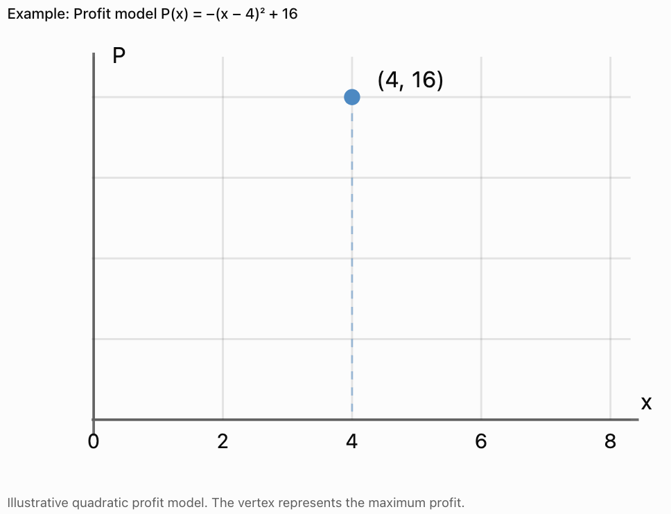
The vertex identifies the maximum or minimum value.

For a profit model, the vertex may identify the quantity that maximises profit.

For a projectile model, it identifies the maximum height and when that height occurs.

The x-Intercepts

The x-intercepts are the input values for which the output equals zero.

Depending on the context, they may represent:

• Times when a projectile is at ground level.

• Break-even quantities in a profit model.

• Dimensions that produce zero area.

The y-Intercept

The y-intercept is the output when the input equals zero.

It may represent:

• Initial height.

• Initial cost.

• An initial measured value.

The Direction of Opening

• An upward-opening parabola has a minimum.

• A downward-opening parabola has a maximum.

Evaluating Whether a Quadratic Model Is Appropriate

A quadratic equation may fit a set of data without necessarily being a good model of the real situation.

Several questions should be considered.

Does the Data Support a Quadratic Relationship?

Look for a curved pattern or approximately constant second differences when the input values are equally spaced.

Does the Model Make Physical Sense?

A model must be consistent with the situation.

For example, a model predicting a negative physical length is not meaningful.

Is the Domain Appropriate?

Some mathematical inputs are impossible in real life.

For example:

• Time may be restricted to nonnegative values.

• Production quantities may need to be whole numbers.

• A garden width must be positive and smaller than the available half-perimeter.

Are the Assumptions Reasonable?

A projectile model may ignore air resistance.

A business model may assume demand follows a simple equation.

A braking model may assume constant deceleration.

How Accurate Are the Predictions?

Compare predicted values with actual observations.

A useful model should provide predictions accurate enough for its intended purpose.

Residuals and Model Accuracy

A residual is the difference between an observed value and the value predicted by a model.

Residual = observed value − predicted value

Example

A quadratic model predicts a height of 12 metres.

The measured height is 11.6 metres.

Residual:

11.6 − 12 = −0.4 m

The model overestimated the height by 0.4 metres.

Interpreting Residuals

• Small residuals suggest the model fits the observations closely.

• Large residuals suggest the model may not fit well.

• A consistent pattern in residuals suggests that another type of model might be more appropriate.

Important Observation

A model can fit existing data closely and still make poor predictions outside the measured range.

Interpolation and Extrapolation

Mathematical models are often used to predict unknown values.

Interpolation

Interpolation means predicting a value within the range of observed data.

For example, if heights were measured at 1, 2, and 3 seconds, estimating the height at 2.5 seconds is interpolation.

Extrapolation

Extrapolation means predicting a value outside the observed range.

For example, using the same measurements to predict the height after 20 seconds is extrapolation.

Important Observation

Extrapolation is generally less reliable because the original mathematical relationship may no longer apply.

A projectile may already have landed, or a business model may no longer describe market behaviour at extremely high production levels.

A Step-by-Step Modelling Process

A reliable modelling process can be applied to many quadratic situations.

Common Mistakes

• Failing to define variables: Always state what the input and output represent.

• Forgetting units: A height of 12 is incomplete without specifying metres, centimetres, or another unit.

• Assuming every curved graph is quadratic: Other functions can also produce curved graphs.

• Ignoring the domain: Mathematical solutions may be impossible in the real situation.

• Confusing maximum and minimum values: Use the sign of a to determine the direction of opening.

• Interpreting a decimal as a whole number: A quantity of 12.5 products may require checking neighbouring integers.

• Assuming a model is perfectly accurate: Real-world measurements and simplified assumptions introduce uncertainty.

• Using extrapolation carelessly: Predictions far outside the measured range may be unreliable.

• Confusing the vertex coordinates: The x-coordinate identifies the input at the optimum; the y-coordinate identifies the maximum or minimum output.

• Ignoring the meaning of intercepts: Each intercept should be interpreted in the context of the problem.

Key Terms

• Mathematical Model: An equation, graph, or other mathematical representation of a real-world situation.

• Quadratic Model: A model based on a quadratic function.

• Independent Variable: The input variable.

• Dependent Variable: The output variable.

• Parabola: The graph of a quadratic function.

• Vertex: The maximum or minimum point of a parabola.

• Maximum Value: The greatest output of a function over its domain.

• Minimum Value: The smallest output of a function over its domain.

• Axis of Symmetry: The vertical line passing through the vertex of a parabola.

• Standard Form: A quadratic equation written as y = ax² + bx + c.

• Vertex Form: A quadratic equation written as y = a(x − h)² + k.

• Factored Form: A quadratic equation written as y = a(x − r₁)(x − r₂).

• Domain: The set of permitted input values.

• Range: The set of possible output values.

• First Differences: Differences between consecutive output values.

• Second Differences: Differences between consecutive first differences.

• Residual: The difference between an observed value and a predicted value.

• Interpolation: Estimating a value within the observed data range.

• Extrapolation: Predicting a value outside the observed data range.

• Assumption: A condition accepted as true when constructing a model.

• Constraint: A restriction on the possible values in a model.

• Optimisation: Finding the maximum or minimum value of a quantity.

• Revenue: Money received from sales before subtracting costs.

• Profit: Revenue minus costs.

Key Takeaways

• Quadratic models represent relationships involving squared variables.

• Quadratic graphs are parabolas.

• Projectile motion, garden area, business revenue, and some engineering designs can be modelled using quadratic functions.

• Choosing appropriate variables is essential.

• Variables should be defined with meaningful units.

• Standard form is useful for identifying initial values and coefficients.

• Vertex form is useful for identifying maximum and minimum values.

• Factored form is useful for identifying zeros.

• Constant second differences indicate an exact quadratic pattern when inputs are equally spaced.

• The vertex often represents an important optimum in a real-world situation.

• Domain restrictions must be considered when interpreting solutions.

• Mathematical answers must be checked for practical meaning.

• Real-world models depend on assumptions and may have limitations.

• Residuals help evaluate how closely a model matches observations.

• Extrapolation should be treated cautiously.

Check Your Understanding

Recognising Quadratic Situations

1. Give two real-world situations that can be modelled by quadratic functions.

2. Explain why projectile height can be modelled by a quadratic function.

3. Is a relationship with constant first differences linear or quadratic?

4. What pattern in second differences suggests a quadratic relationship?

5. Explain why not every curved graph is quadratic.

Variables and Equations

6. In h(t) = −5t² + 15t + 2, identify the independent and dependent variables.

7. What does the constant 2 represent in the model above?

8. A rectangle has perimeter 30 m. Write its length in terms of width w.

9. Write a quadratic equation for the area of that rectangle.

10. Explain why variables should include units.

Interpreting Models

11. Find the vertex of P(x) = −2(x − 5)² + 100.

12. Interpret the vertex in a profit model.

13. Find the maximum height of h(t) = −5(t − 3)² + 45.

14. Determine the range of y = (x − 2)² + 4 for all real x.

15. Explain what an x-intercept might represent in a projectile model.

Evaluating Models

16. Why might a quadratic model produce unrealistic predictions outside its intended domain?

17. What is a residual?

18. Calculate the residual if the observed value is 18 and the predicted value is 20.

19. Explain the difference between interpolation and extrapolation.

20. Give two reasons a quadratic model might not accurately represent real-world data.

Answer Key

Extended Challenge

1. A ball's height is h(t) = −5t² + 30t + 2. Find its maximum height and the time at which it occurs.

2. Determine when the ball in Question 1 reaches ground level. Give the physically meaningful answer.

3. A rectangular garden has a perimeter of 60 m. Write an area function in terms of its width.

4. Determine the dimensions that maximise the garden's area.

5. A company's revenue is R(x) = −4x² + 80x. Find the quantity that maximises revenue.

6. Determine the maximum revenue.

7. A parabolic arch has vertex (0, 12) and passes through (4, 4). Find its equation.

8. Determine the horizontal positions where the arch reaches ground level.

9. Construct a quadratic model for the data points (0, 1), (1, 4), and (2, 9).

10. Explain how you could test whether this model is suitable for additional measurements.

Final Investigation: Designing a Garden

A school wants to build a rectangular garden using 48 metres of fencing.

The goal is to create the largest possible planting area.

Complete the investigation.

1. Define suitable variables for the width, length, and area.

2. Write the perimeter equation.

3. Rearrange the equation to express length in terms of width.

4. Write the area equation.

5. Expand the area equation into standard quadratic form.

6. Identify the coefficients a, b, and c.

7. Explain why the parabola opens downward.

8. Determine the vertex.

9. Interpret the vertex in the context of the garden.

10. Calculate the maximum area.

11. Determine the garden dimensions that produce this area.

12. Construct a table of values for widths of 4, 6, 8, 10, 12, 14, 16, 18, and 20 metres.

13. Graph the area function.

14. Identify the axis of symmetry.

15. Explain why two different widths can sometimes produce the same area.

16. Determine the physically meaningful domain.

17. Explain why negative widths are not acceptable.

18. Describe two assumptions made in the model.

19. Explain how the model would change if one side of the garden did not require fencing.

20. Write a conclusion evaluating the usefulness and limitations of the quadratic model.

Investigation Check

The area equation should be:

A(w) = −w² + 24w

The vertex is:

(12, 144)

Therefore, the maximum area is 144 m², achieved with a square garden measuring 12 m by 12 m.

The physically meaningful domain is:

0 < w < 24