Applications of Quadratic Functions
| Site: | Young Education |
| Course: | Quadratic Functions |
| Book: | Applications of Quadratic Functions |
| Printed by: | Guest user |
| Date: | Monday, 9 November 2026, 4:40 PM |
1. Modelling Real-World Situations
Learning outcomes
- I can identify situations modelled by quadratic functions.
- I can interpret quadratic models.
- I can determine appropriate variables.
- I can create simple quadratic models.
- I can evaluate whether a quadratic model is appropriate.
Modelling Real-World Situations with Quadratic Functions
Introduction
Mathematics helps us describe, understand, and predict events in the real world. One particularly useful type of mathematical relationship is a quadratic function.
Quadratic functions are used to model situations involving curved paths, maximum and minimum values, changing areas, profits, costs, and many other relationships.
For example:
-
The height of a ball thrown into the air changes over time.
-
The area of a rectangular garden depends on its dimensions.
-
The profit earned by a business may increase and then decrease as production changes.
-
The braking distance of a vehicle increases approximately with the square of its speed under suitable conditions.
-
The shape of a parabolic arch can be described using a quadratic equation.
A quadratic model allows us to represent these situations mathematically and use equations, graphs, and tables to make predictions.
However, not every real-world relationship is quadratic. An important part of mathematical modelling is deciding whether a quadratic function is an appropriate representation of the situation.


What Is a Quadratic Model?
A quadratic model is a mathematical equation that uses a quadratic function to represent a real-world relationship.
The general form is:
y = ax² + bx + c
where:
-
x is the independent variable.
-
y is the dependent variable.
-
a, b, and c are constants.
-
a ≠ 0.
The independent variable represents the quantity we choose, measure, or control.
The dependent variable represents the quantity that changes in response.
Example
Suppose the height of a ball is modelled by:
h(t) = −5t² + 20t + 2
where:
-
t represents time in seconds.
-
h represents height in metres.
The height depends on the time, so time is the independent variable and height is the dependent variable.
Why Is This Quadratic?
The equation contains a squared variable, t².
The highest power of the independent variable is 2.
Therefore, it is a quadratic function.
Recognising Situations That May Be Quadratic
Quadratic models are useful when the relationship between two variables forms a parabola.
Common characteristics include:
-
A quantity increases and then decreases.
-
A quantity decreases and then increases.
-
There is a maximum or minimum value.
-
The rate of change increases or decreases at a constant rate.
-
The relationship involves multiplying two changing quantities.
-
A physical relationship involves the square of a variable.
Examples
|
Situation |
Possible variables |
Why quadratic? |
|---|---|---|
|
Projectile motion |
Time and height |
Constant vertical acceleration produces a t² term |
|
Garden area |
Width and area |
Length and width may both change |
|
Business profit |
Quantity and profit |
A linear demand relationship can produce quadratic revenue |
|
Braking distance |
Speed and distance |
Idealised stopping distance is proportional to speed squared |
|
Parabolic arch |
Horizontal position and height |
Shape can be represented by a parabola |
Important Observation
A real-world situation should not be classified as quadratic simply because it involves a maximum or minimum. The equation, data, or underlying relationship must support a quadratic model.
Choosing Appropriate Variables
Before creating a mathematical model, we must decide what the variables represent.
A good model uses clearly defined quantities and units.
Independent Variable
The independent variable is the input.
It is often represented by x or t.
Examples include:
-
Time in seconds
-
Distance in metres
-
Number of products manufactured
-
Width of a garden
-
Speed of a vehicle
Dependent Variable
The dependent variable is the output.
Its value depends on the independent variable.
Examples include:
-
Height in metres
-
Area in square metres
-
Profit in dollars
-
Braking distance in metres
-
Revenue in dollars
Example
A rectangular garden has a fixed perimeter of 40 metres.
We want to investigate how its area changes as its width changes.
Choose:
w = width of the garden in metres
A = area of the garden in square metres
The width is the independent variable.
The area is the dependent variable.
Important Observation
Always include units when defining variables. This makes the model easier to interpret and helps prevent calculation errors.
The Three Common Forms of Quadratic Models
Quadratic functions can be written in several forms. Each form is useful for a different purpose.
Standard Form
y = ax² + bx + c
This form is useful for identifying the leading coefficient and initial value when x = 0.
For example:
h(t) = −5t² + 20t + 2
The initial height is:
h(0) = 2 metres
Vertex Form
y = a(x − h)² + k
This form is useful for identifying maximum or minimum values.
For example:
P(x) = −2(x − 10)² + 200
The maximum profit is 200 when x = 10.
Factored Form
y = a(x − r₁)(x − r₂)
This form is useful for identifying the zeros of a function.
For example:
A(x) = x(20 − x)
The area is zero when x = 0 or x = 20.
Comparison
|
Form |
Most useful information |
|---|---|
|
Standard |
Coefficients and value at x = 0 |
|
Vertex |
Maximum or minimum value |
|
Factored |
Zeros and intercepts |
Modelling Projectile Motion
One of the most familiar applications of quadratic functions is projectile motion.
When an object is launched into the air, gravity causes its vertical velocity to change.
Ignoring air resistance and assuming constant gravitational acceleration, its height can be modelled by a quadratic function.

General Height Model
h(t) = −0.5gt² + v₀t + h₀
where:
-
h(t) = height at time t, in metres
-
g = gravitational acceleration, approximately 9.8 m/s²
-
v₀ = initial vertical velocity, in m/s
-
h₀ = initial height, in metres
-
t = time, in seconds
Near Earth's surface, this is approximately:
h(t) = −4.9t² + v₀t + h₀
For simpler classroom calculations, we may use:
h(t) = −5t² + v₀t + h₀
Worked Example
A ball is thrown upward from a platform 2 metres high with an initial vertical velocity of 20 m/s.
Its approximate height is:
h(t) = −5t² + 20t + 2
Finding the Height After One Second
Substitute t = 1:
h(1) = −5(1)² + 20(1) + 2
h(1) = −5 + 20 + 2
h(1) = 17 metres
Finding the Maximum Height
The time coordinate of the vertex is:
t = −b/(2a)
Here:
a = −5
b = 20
t = −20/[2(−5)]
t = 2 seconds
Now calculate the height:
h(2) = −5(2)² + 20(2) + 2
h(2) = −20 + 40 + 2
Maximum height = 22 metres
Interpretation
The ball reaches its maximum height of 22 metres after 2 seconds.
The graph opens downward because the coefficient of t² is negative.
Limitations
The model assumes:
-
Constant gravitational acceleration
-
Negligible air resistance
-
A fixed vertical reference point
It may become inaccurate if air resistance is significant or the object experiences additional forces.
Modelling the Area of a Garden
Quadratic functions are useful when two dimensions change while a total length remains fixed.

Example
A gardener has 40 metres of fencing and wants to enclose a rectangular garden.
What dimensions produce the maximum area?
Step 1: Define Variables
Let:
w = width in metres
l = length in metres
A = area in square metres
Step 2: Write the Perimeter Equation
The perimeter is:
2w + 2l = 40
Divide by 2:
w + l = 20
Rearrange:
l = 20 − w
Step 3: Write the Area Equation
Area of a rectangle:
A = lw
Substitute l = 20 − w:
A = w(20 − w)
Expand:
A(w) = −w² + 20w
This is a quadratic model.
Step 4: Find the Maximum Area
a = −1
b = 20
The vertex occurs at:
w = −20/[2(−1)]
w = 10 metres
Find the length:
l = 20 − 10
l = 10 metres
Find the area:
A = 10 × 10
Maximum area = 100 m²
Interpretation
The largest rectangular garden possible with 40 metres of fencing is a square measuring 10 m by 10 m.
Valid Domain
Because the dimensions must be positive:
0 < w < 20
Values outside this interval do not represent a physically possible garden.
Modelling Business Revenue and Profit
Quadratic functions can describe how revenue or profit changes with production and pricing.
Example: Revenue
A business estimates that the selling price of a product decreases as more products are sold.
Suppose the price is:
p = 50 − 2x
where:
-
p = price per item in dollars
-
x = number of items sold
Revenue is:
R = price × quantity
Therefore:
R(x) = x(50 − 2x)
Expand:
R(x) = −2x² + 50x
Finding Maximum Revenue
The vertex occurs at:
x = −b/(2a)
x = −50/[2(−2)]
x = 12.5
Substitute:
R(12.5) = −2(12.5)² + 50(12.5)
R(12.5) = −312.5 + 625
R(12.5) = $312.50
Interpretation
The continuous mathematical model predicts maximum revenue at x = 12.5.
However, products are normally sold in whole numbers.
We should compare x = 12 and x = 13:
R(12) = $312
R(13) = $312
Therefore, the maximum revenue for whole-item sales is $312, achieved by selling either 12 or 13 items.
Important Observation
A mathematical model may produce a solution that is not practical in the real world.
The answer must be interpreted using the situation's constraints.
Modelling Braking Distance
A vehicle's braking distance depends on several factors, including speed, road conditions, tyres, and braking force.
Under simplified conditions where the braking deceleration is constant, braking distance is proportional to the square of the initial speed.

Example
Suppose a simplified braking-distance model is:
d(v) = 0.01v²
where:
-
d = braking distance in metres
-
v = initial speed in km/h
Calculating Braking Distance
At 40 km/h:
d(40) = 0.01(40)²
d(40) = 16 m
At 80 km/h:
d(80) = 0.01(80)²
d(80) = 64 m
Comparison
|
Speed (km/h) |
Braking distance (m) |
|---|---|
|
20 |
4 |
|
40 |
16 |
|
60 |
36 |
|
80 |
64 |
|
100 |
100 |
Interpretation
Doubling the speed from 40 km/h to 80 km/h increases the predicted braking distance from 16 metres to 64 metres.
Doubling speed quadruples braking distance in this model.
This happens because:
(2v)² = 4v²
Limitations
The coefficient 0.01 is illustrative, not a universal braking constant. Actual braking distances depend on road conditions, tyres, braking systems, and other factors. The model also excludes the distance travelled during the driver's reaction time.
Modelling Parabolic Arches
Quadratic functions can describe curved structures such as bridges, gateways, and architectural arches.

Example
A parabolic arch is 12 metres wide and 9 metres high at its centre.
We want to create an equation describing the shape.
Step 1: Choose a Coordinate System
Place the origin at ground level directly beneath the centre of the arch.
The highest point is:
(0, 9)
The arch meets the ground at:
(−6, 0) and (6, 0)
Step 2: Use Vertex Form
The equation is:
y = a(x − h)² + k
Since the vertex is (0, 9):
y = ax² + 9
Step 3: Substitute a Known Point
Use (6, 0):
0 = a(6)² + 9
0 = 36a + 9
36a = −9
a = −0.25
Step 4: Write the Model
y = −0.25x² + 9
Step 5: Interpret
The negative coefficient means the arch opens downward.
The maximum height is 9 metres.
The physically relevant domain is:
−6 ≤ x ≤ 6
The range of the physical arch is:
0 ≤ y ≤ 9
Important Observation
Although the quadratic function extends indefinitely, the actual arch exists only within a restricted domain.
Creating Quadratic Models from Tables
Sometimes a mathematical model must be created from observed data rather than a description.
Consider the following values:
|
x |
y |
|---|---|
|
0 |
2 |
|
1 |
5 |
|
2 |
10 |
|
3 |
17 |
|
4 |
26 |
Step 1: Calculate First Differences
Subtract consecutive y-values:
5 − 2 = 3
10 − 5 = 5
17 − 10 = 7
26 − 17 = 9
First differences:
3, 5, 7, 9
These are not constant, so the data are not linear.
Step 2: Calculate Second Differences
5 − 3 = 2
7 − 5 = 2
9 − 7 = 2
Second differences:
2, 2, 2
The second differences are constant.
For equally spaced x-values, this is evidence of a quadratic relationship.
Step 3: Write a General Equation
y = ax² + bx + c
When x = 0, y = 2.
Therefore:
c = 2
For unit spacing, the constant second difference equals 2a.
2a = 2
a = 1
Use the point (1, 5):
5 = 1 + b + 2
b = 2
Final Model
y = x² + 2x + 2
Step 4: Check
At x = 3:
y = 3² + 2(3) + 2
y = 9 + 6 + 2
y = 17
The equation matches the table.
Important Observation
Constant second differences identify an exact quadratic pattern in equally spaced, error-free data. Real measurements may contain errors, so their second differences may only be approximately constant.
Comparing Linear and Quadratic Models
Not every relationship is quadratic.
A linear model has a constant rate of change.
A quadratic model has a rate of change that changes linearly.
Example
Compare:
Linear: y = 3x + 2
Quadratic: y = x² + 2
|
x |
Linear |
Quadratic |
|---|---|---|
|
0 |
2 |
2 |
|
1 |
5 |
3 |
|
2 |
8 |
6 |
|
3 |
11 |
11 |
|
4 |
14 |
18 |
|
5 |
17 |
27 |
Linear Relationship
The output increases by 3 for every increase of 1 in x.
First differences are constant.
Quadratic Relationship
The output increases by progressively larger amounts.
Second differences are constant.
Important Conclusion
The pattern in the data helps determine which type of model is appropriate.
Interpreting Quadratic Graphs
A quadratic graph can reveal useful information about a real-world situation.
The Vertex
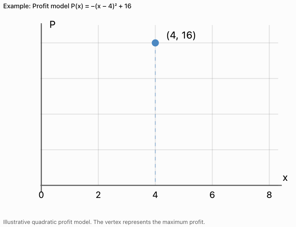
The vertex identifies the maximum or minimum value.
For a profit model, the vertex may identify the quantity that maximises profit.
For a projectile model, it identifies the maximum height and when that height occurs.
The x-Intercepts
The x-intercepts are the input values for which the output equals zero.
Depending on the context, they may represent:
-
Times when a projectile is at ground level.
-
Break-even quantities in a profit model.
-
Dimensions that produce zero area.
The y-Intercept
The y-intercept is the output when the input equals zero.
It may represent:
-
Initial height.
-
Initial cost.
-
An initial measured value.
The Direction of Opening
-
An upward-opening parabola has a minimum.
-
A downward-opening parabola has a maximum.
Evaluating Whether a Quadratic Model Is Appropriate
A quadratic equation may fit a set of data without necessarily being a good model of the real situation.
Several questions should be considered.
Does the Data Support a Quadratic Relationship?
Look for a curved pattern or approximately constant second differences when the input values are equally spaced.
Does the Model Make Physical Sense?
A model must be consistent with the situation.
For example, a model predicting a negative physical length is not meaningful.
Is the Domain Appropriate?
Some mathematical inputs are impossible in real life.
For example:
-
Time may be restricted to nonnegative values.
-
Production quantities may need to be whole numbers.
-
A garden width must be positive and smaller than the available half-perimeter.
Are the Assumptions Reasonable?
A projectile model may ignore air resistance.
A business model may assume demand follows a simple equation.
A braking model may assume constant deceleration.
How Accurate Are the Predictions?
Compare predicted values with actual observations.
A useful model should provide predictions accurate enough for its intended purpose.
Residuals and Model Accuracy
A residual is the difference between an observed value and the value predicted by a model.
Residual = observed value − predicted value
Example
A quadratic model predicts a height of 12 metres.
The measured height is 11.6 metres.
Residual:
11.6 − 12 = −0.4 m
The model overestimated the height by 0.4 metres.
Interpreting Residuals
-
Small residuals suggest the model fits the observations closely.
-
Large residuals suggest the model may not fit well.
-
A consistent pattern in residuals suggests that another type of model might be more appropriate.
Important Observation
A model can fit existing data closely and still make poor predictions outside the measured range.
Interpolation and Extrapolation
Mathematical models are often used to predict unknown values.
Interpolation
Interpolation means predicting a value within the range of observed data.
For example, if heights were measured at 1, 2, and 3 seconds, estimating the height at 2.5 seconds is interpolation.
Extrapolation
Extrapolation means predicting a value outside the observed range.
For example, using the same measurements to predict the height after 20 seconds is extrapolation.
Important Observation
Extrapolation is generally less reliable because the original mathematical relationship may no longer apply.
A projectile may already have landed, or a business model may no longer describe market behaviour at extremely high production levels.
A Step-by-Step Modelling Process
A reliable modelling process can be applied to many quadratic situations.
-
Understand the situation. Identify what is changing and what needs to be calculated.
-
Define variables. State what each variable represents and include units.
-
Identify relationships. Use the information provided to construct an equation.
-
Create the model. Write a quadratic function in an appropriate form.
-
Solve or graph. Find relevant values, intercepts, or the vertex.
-
Interpret the results. Explain what the mathematical answers mean.
-
Evaluate the model. Check assumptions, domain restrictions, accuracy, and limitations.
Common Mistakes
-
Failing to define variables: Always state what the input and output represent.
-
Forgetting units: A height of 12 is incomplete without specifying metres, centimetres, or another unit.
-
Assuming every curved graph is quadratic: Other functions can also produce curved graphs.
-
Ignoring the domain: Mathematical solutions may be impossible in the real situation.
-
Confusing maximum and minimum values: Use the sign of a to determine the direction of opening.
-
Interpreting a decimal as a whole number: A quantity of 12.5 products may require checking neighbouring integers.
-
Assuming a model is perfectly accurate: Real-world measurements and simplified assumptions introduce uncertainty.
-
Using extrapolation carelessly: Predictions far outside the measured range may be unreliable.
-
Confusing the vertex coordinates: The x-coordinate identifies the input at the optimum; the y-coordinate identifies the maximum or minimum output.
-
Ignoring the meaning of intercepts: Each intercept should be interpreted in the context of the problem.
Key Terms
-
Mathematical Model: An equation, graph, or other mathematical representation of a real-world situation.
-
Quadratic Model: A model based on a quadratic function.
-
Independent Variable: The input variable.
-
Dependent Variable: The output variable.
-
Parabola: The graph of a quadratic function.
-
Vertex: The maximum or minimum point of a parabola.
-
Maximum Value: The greatest output of a function over its domain.
-
Minimum Value: The smallest output of a function over its domain.
-
Axis of Symmetry: The vertical line passing through the vertex of a parabola.
-
Standard Form: A quadratic equation written as y = ax² + bx + c.
-
Vertex Form: A quadratic equation written as y = a(x − h)² + k.
-
Factored Form: A quadratic equation written as y = a(x − r₁)(x − r₂).
-
Domain: The set of permitted input values.
-
Range: The set of possible output values.
-
First Differences: Differences between consecutive output values.
-
Second Differences: Differences between consecutive first differences.
-
Residual: The difference between an observed value and a predicted value.
-
Interpolation: Estimating a value within the observed data range.
-
Extrapolation: Predicting a value outside the observed data range.
-
Assumption: A condition accepted as true when constructing a model.
-
Constraint: A restriction on the possible values in a model.
-
Optimisation: Finding the maximum or minimum value of a quantity.
-
Revenue: Money received from sales before subtracting costs.
-
Profit: Revenue minus costs.
Key Takeaways
-
Quadratic models represent relationships involving squared variables.
-
Quadratic graphs are parabolas.
-
Projectile motion, garden area, business revenue, and some engineering designs can be modelled using quadratic functions.
-
Choosing appropriate variables is essential.
-
Variables should be defined with meaningful units.
-
Standard form is useful for identifying initial values and coefficients.
-
Vertex form is useful for identifying maximum and minimum values.
-
Factored form is useful for identifying zeros.
-
Constant second differences indicate an exact quadratic pattern when inputs are equally spaced.
-
The vertex often represents an important optimum in a real-world situation.
-
Domain restrictions must be considered when interpreting solutions.
-
Mathematical answers must be checked for practical meaning.
-
Real-world models depend on assumptions and may have limitations.
-
Residuals help evaluate how closely a model matches observations.
-
Extrapolation should be treated cautiously.
Check Your Understanding
Recognising Quadratic Situations
-
Give two real-world situations that can be modelled by quadratic functions.
-
Explain why projectile height can be modelled by a quadratic function.
-
Is a relationship with constant first differences linear or quadratic?
-
What pattern in second differences suggests a quadratic relationship?
-
Explain why not every curved graph is quadratic.
Variables and Equations
-
In h(t) = −5t² + 15t + 2, identify the independent and dependent variables.
-
What does the constant 2 represent in the model above?
-
A rectangle has perimeter 30 m. Write its length in terms of width w.
-
Write a quadratic equation for the area of that rectangle.
-
Explain why variables should include units.
Interpreting Models
-
Find the vertex of P(x) = −2(x − 5)² + 100.
-
Interpret the vertex in a profit model.
-
Find the maximum height of h(t) = −5(t − 3)² + 45.
-
Determine the range of y = (x − 2)² + 4 for all real x.
-
Explain what an x-intercept might represent in a projectile model.
Evaluating Models
-
Why might a quadratic model produce unrealistic predictions outside its intended domain?
-
What is a residual?
-
Calculate the residual if the observed value is 18 and the predicted value is 20.
-
Explain the difference between interpolation and extrapolation.
-
Give two reasons a quadratic model might not accurately represent real-world data.
Answer Key
|
Question |
Answer |
|---|---|
|
1 |
Examples: projectile motion and garden area |
|
2 |
Constant vertical acceleration produces a squared-time term |
|
3 |
Linear |
|
4 |
Constant second differences for equally spaced inputs |
|
5 |
Many other functions produce curves |
|
6 |
Independent: time t; dependent: height h |
|
7 |
Initial height of 2 m |
|
8 |
l = 15 − w |
|
9 |
A(w) = −w² + 15w |
|
10 |
Units explain what the values represent |
|
11 |
(5, 100) |
|
12 |
Maximum profit of 100 at input 5 |
|
13 |
45 |
|
14 |
y ≥ 4 |
|
15 |
A time when the projectile is at height zero |
|
16 |
The assumptions or physical conditions may no longer apply |
|
17 |
Observed value minus predicted value |
|
18 |
−2 |
|
19 |
Interpolation is within the observed range; extrapolation is outside |
|
20 |
Measurement errors, unrealistic assumptions, or an unsuitable relationship |
Extended Challenge
-
A ball's height is h(t) = −5t² + 30t + 2. Find its maximum height and the time at which it occurs.
-
Determine when the ball in Question 1 reaches ground level. Give the physically meaningful answer.
-
A rectangular garden has a perimeter of 60 m. Write an area function in terms of its width.
-
Determine the dimensions that maximise the garden's area.
-
A company's revenue is R(x) = −4x² + 80x. Find the quantity that maximises revenue.
-
Determine the maximum revenue.
-
A parabolic arch has vertex (0, 12) and passes through (4, 4). Find its equation.
-
Determine the horizontal positions where the arch reaches ground level.
-
Construct a quadratic model for the data points (0, 1), (1, 4), and (2, 9).
-
Explain how you could test whether this model is suitable for additional measurements.
Final Investigation: Designing a Garden
A school wants to build a rectangular garden using 48 metres of fencing.
The goal is to create the largest possible planting area.
Complete the investigation.
-
Define suitable variables for the width, length, and area.
-
Write the perimeter equation.
-
Rearrange the equation to express length in terms of width.
-
Write the area equation.
-
Expand the area equation into standard quadratic form.
-
Identify the coefficients a, b, and c.
-
Explain why the parabola opens downward.
-
Determine the vertex.
-
Interpret the vertex in the context of the garden.
-
Calculate the maximum area.
-
Determine the garden dimensions that produce this area.
-
Construct a table of values for widths of 4, 6, 8, 10, 12, 14, 16, 18, and 20 metres.
-
Graph the area function.
-
Identify the axis of symmetry.
-
Explain why two different widths can sometimes produce the same area.
-
Determine the physically meaningful domain.
-
Explain why negative widths are not acceptable.
-
Describe two assumptions made in the model.
-
Explain how the model would change if one side of the garden did not require fencing.
-
Write a conclusion evaluating the usefulness and limitations of the quadratic model.
Investigation Check
The area equation should be:
A(w) = −w² + 24w
The vertex is:
(12, 144)
Therefore, the maximum area is 144 m², achieved with a square garden measuring 12 m by 12 m.
The physically meaningful domain is:
0 < w < 24
2. Projectile Motion
Learning outcomes
- I can recognise projectile motion as quadratic.
- I can interpret height-time graphs.
- I can determine maximum height.
- I can determine when an object reaches the ground.
- I can solve projectile problems using quadratic functions.
Projectile Motion
Introduction
When a ball is thrown, a basketball is shot toward a hoop, or a rocket launches into the air, the object follows a path influenced by gravity.
This type of motion is called projectile motion.
Projectile motion is an important application of quadratic functions because the height of an object changes with time according to a quadratic relationship, provided gravitational acceleration is constant and air resistance is negligible.
Quadratic models allow us to answer questions such as:
-
How high will the object travel?
-
How long will it take to reach its maximum height?
-
When will the object return to the ground?
-
What will its height be at a particular time?
-
How can a height-time graph help us predict its motion?


What Is Projectile Motion?
Projectile motion is the movement of an object that has been launched and then moves under the influence of gravity, assuming other forces such as air resistance can be ignored.
Examples include:
-
A basketball travelling toward a hoop.
-
A ball thrown vertically upward.
-
A football kicked through the air.
-
Water leaving a fountain.
-
A stone thrown from a cliff.
A projectile may move both horizontally and vertically.
Horizontal Motion
In ideal projectile motion, horizontal velocity remains constant because there is no horizontal acceleration.
Vertical Motion
Vertical velocity changes because gravity accelerates the object downward.
Near Earth's surface, gravitational acceleration is approximately:
g = 9.8 m/s²
For simpler calculations, we often use:
g ≈ 10 m/s²
Important Observation
Even when a projectile moves horizontally and vertically, its height as a function of time is quadratic.
Its trajectory through space is also parabolic under the same ideal assumptions, provided it has a nonzero horizontal velocity.
The Quadratic Model for Projectile Height
The vertical position of a projectile can be described using:
h(t) = −0.5gt² + v₀t + h₀
where:
-
h(t) = height at time t, in metres
-
t = time after launch, in seconds
-
g = gravitational acceleration, in m/s²
-
v₀ = initial vertical velocity, in m/s
-
h₀ = initial height, in metres
Using g ≈ 10 m/s²:
h(t) = −5t² + v₀t + h₀
This has the same structure as the standard quadratic function:
y = ax² + bx + c
|
Quadratic term |
Projectile interpretation |
|---|---|
|
a |
Half the vertical acceleration, −g/2 |
|
b |
Initial vertical velocity |
|
c |
Initial height |
|
x |
Time |
|
y |
Height |
Why Is the Coefficient of t² Negative?
Gravity accelerates the projectile downward.
Because upward is defined as positive, the vertical acceleration is negative.
Therefore, the height-time parabola opens downward.
Understanding the Shape of Projectile Motion
A typical projectile follows a curved path.

During its flight:
-
The projectile begins at its initial height.
-
If launched upward, it rises while slowing vertically.
-
It reaches a maximum height.
-
Its vertical velocity becomes zero momentarily.
-
It begins moving downward.
-
Its downward vertical speed increases as it falls.
Important Distinction
At the maximum height, the vertical velocity is zero, but the acceleration remains downward.
If the projectile has horizontal velocity, it is still moving horizontally at the highest point.
Interpreting Height-Time Graphs
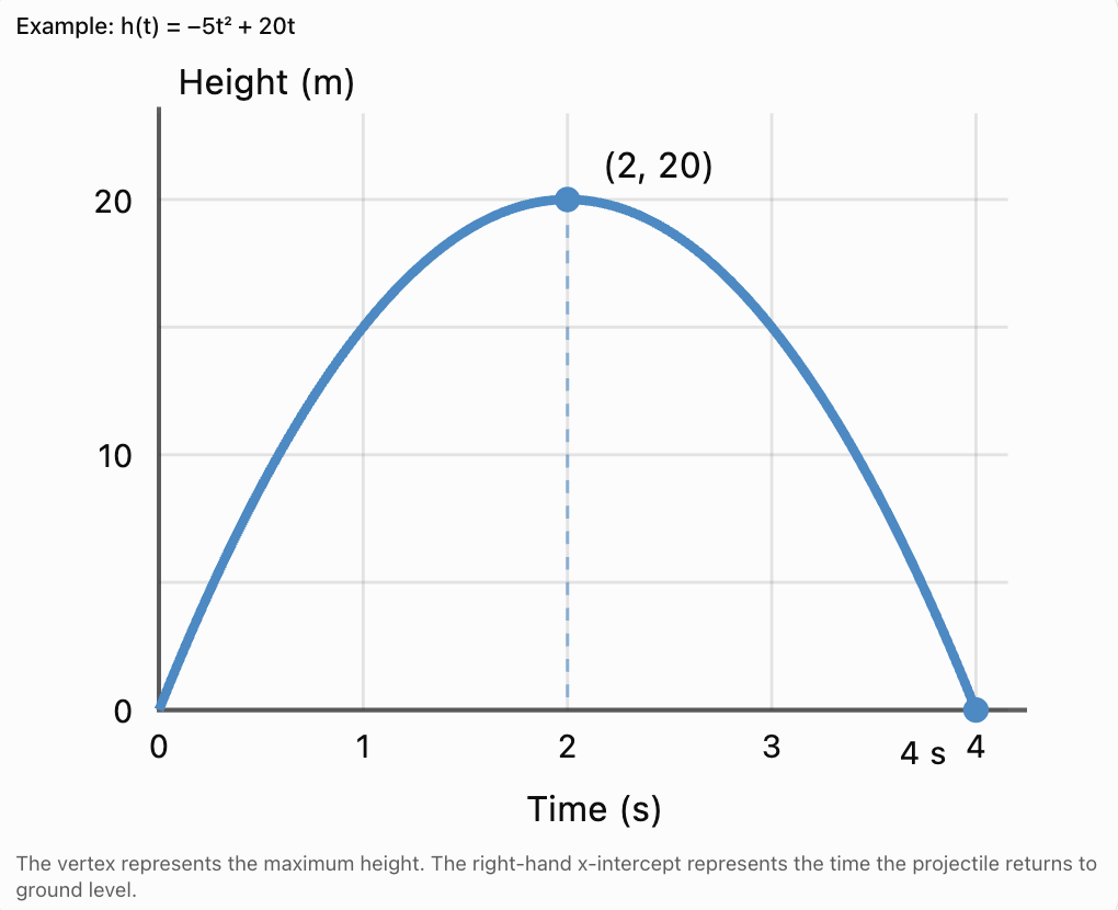
A height-time graph shows how the vertical position of a projectile changes over time.
Important Features
The y-intercept: Represents the initial height.
The vertex: Represents the maximum height and the time it occurs.
The x-intercepts: Represent times when the height is zero.
The increasing section: Represents the projectile rising.
The decreasing section: Represents the projectile falling.
Important Observation
The horizontal axis represents time, not horizontal distance.
A height-time graph is different from a diagram showing the actual trajectory of the projectile through space.
Exploring Projectile Motion
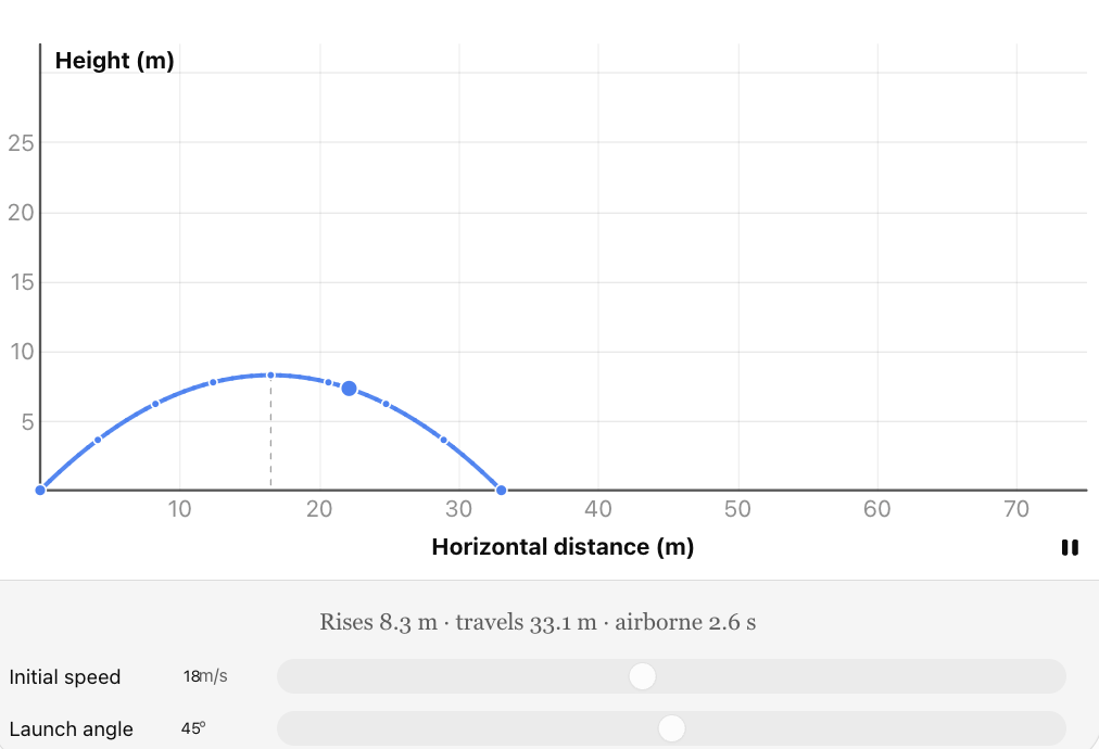
Explore how changing the launch speed and angle affects the projectile's maximum height, flight time, and horizontal range.
In this ideal model, the projectile launches and lands at the same height. The motion assumes constant gravity and negligible air resistance.
Calculating Height at a Particular Time
Consider a ball thrown upward from a height of 2 metres.
Its height is modelled by:
h(t) = −5t² + 20t + 2
Finding the Height After One Second
Substitute t = 1:
h(1) = −5(1)² + 20(1) + 2
h(1) = −5 + 20 + 2
h(1) = 17 m
Finding the Height After Three Seconds
Substitute t = 3:
h(3) = −5(3)² + 20(3) + 2
h(3) = −45 + 60 + 2
h(3) = 17 m
Why Are the Heights Equal?
The projectile is at the same height once while rising and once while falling.
These two times are symmetric around the time at which maximum height occurs.
Finding Maximum Height Using the Vertex
The maximum height of a projectile occurs at the vertex of its height-time parabola.
For:
h(t) = at² + bt + c
the time at the vertex is:
t = −b/(2a)
Worked Example
A ball is launched from ground level.
Its height is:
h(t) = −5t² + 30t
Step 1: Identify the Coefficients
a = −5
b = 30
c = 0
Step 2: Calculate the Time at Maximum Height
t = −30/[2(−5)]
t = −30/−10
t = 3 seconds
Step 3: Calculate Maximum Height
Substitute t = 3:
h(3) = −5(3)² + 30(3)
h(3) = −45 + 90
Maximum height = 45 m
Interpretation
The ball reaches a maximum height of 45 metres after 3 seconds.
Finding Maximum Height Using Vertex Form
Sometimes a projectile equation is already written in vertex form:
h(t) = a(t − p)² + q
For a downward-opening parabola:
-
p = time at maximum height
-
q = maximum height
Example
h(t) = −5(t − 4)² + 80
The vertex is:
(4, 80)
Therefore:
-
Time at maximum height = 4 seconds
-
Maximum height = 80 metres
Important Observation
Vertex form makes the maximum height immediately visible without additional calculations.
Finding When a Projectile Reaches the Ground
A projectile reaches ground level when its height is zero.
Therefore, set:
h(t) = 0
Then solve the quadratic equation.
Worked Example: Factoring
A ball is launched from the ground.
Its height is:
h(t) = −5t² + 20t
Set the height equal to zero:
0 = −5t² + 20t
Factor:
0 = −5t(t − 4)
Therefore:
t = 0 or t = 4
Interpretation
-
t = 0 seconds: The ball begins at ground level.
-
t = 4 seconds: The ball returns to ground level.
Flight time = 4 seconds
Important Observation
When a projectile launches from ground level and returns to the same height, the quadratic equation typically has two physically meaningful times: launch and landing.
Finding Landing Time Using the Quadratic Formula
Not every projectile equation can be factored easily.
In these cases, use the quadratic formula:
t = [−b ± √(b² − 4ac)]/(2a)
Worked Example
A ball is thrown upward from a platform 15 metres above the ground.
Its height is:
h(t) = −5t² + 20t + 15
Find when the ball reaches the ground.
Step 1: Set Height Equal to Zero
0 = −5t² + 20t + 15
Divide by −5:
t² − 4t − 3 = 0
Step 2: Identify the Coefficients
a = 1
b = −4
c = −3
Step 3: Substitute into the Formula
t = [4 ± √(16 + 12)]/2
t = [4 ± √28]/2
t = 2 ± √7
Step 4: Calculate Both Solutions
t ≈ −0.65 seconds
t ≈ 4.65 seconds
Step 5: Interpret
The negative time does not represent a time after launch.
Therefore:
The ball reaches the ground approximately 4.65 seconds after launch.
Important Observation
Mathematical solutions must be checked against the physical situation.
Negative times are generally excluded when time is measured from the instant of launch.
The Relationship Between Maximum Height and Flight Time
When a projectile launches and lands at the same height, its height-time graph is symmetric.
Suppose:
h(t) = −5t² + 40t
Finding Maximum Height
Time at vertex:
t = −40/[2(−5)]
t = 4 seconds
Maximum height:
h(4) = −5(4)² + 40(4)
h(4) = −80 + 160
Maximum height = 80 m
Finding Flight Time
Set h(t) = 0:
0 = −5t² + 40t
0 = −5t(t − 8)
t = 0 or t = 8
Flight time = 8 seconds
Relationship
Time to maximum height = 4 seconds
Total flight time = 8 seconds
Therefore:
Time to maximum height = half the total flight time
This relationship applies when the launch and landing heights are equal, under constant gravitational acceleration and negligible air resistance.
Projectile Motion from Different Starting Heights
Not all projectiles begin at ground level.

Example
A ball is thrown upward from a building 20 metres high.
Its height is:
h(t) = −5t² + 15t + 20
Initial Height
At t = 0:
h(0) = 20
The ball begins 20 metres above the ground.
Maximum Height
t = −15/[2(−5)]
t = 1.5 seconds
Substitute:
h(1.5) = −5(1.5)² + 15(1.5) + 20
h(1.5) = −11.25 + 22.5 + 20
Maximum height = 31.25 m
Landing Time
Set height equal to zero:
0 = −5t² + 15t + 20
Divide by −5:
t² − 3t − 4 = 0
Factor:
(t − 4)(t + 1) = 0
t = 4 or t = −1
The physically meaningful solution is:
t = 4 seconds
Important Observation
When the projectile starts above ground level, the time spent rising is generally not half the total time until it reaches the ground.
Comparing Two Projectile Models
Consider two projectiles:
Projectile A: h₁(t) = −5t² + 20t
Projectile B: h₂(t) = −5t² + 30t
Maximum Height of A
t = −20/[2(−5)] = 2 s
h₁(2) = −5(2)² + 20(2)
Maximum height = 20 m
Maximum Height of B
t = −30/[2(−5)] = 3 s
h₂(3) = −5(3)² + 30(3)
Maximum height = 45 m
Comparison
|
Property |
Projectile A |
Projectile B |
|---|---|---|
|
Initial height |
0 m |
0 m |
|
Initial vertical velocity |
20 m/s |
30 m/s |
|
Time to maximum height |
2 s |
3 s |
|
Maximum height |
20 m |
45 m |
|
Total flight time |
4 s |
6 s |
Interpretation
Projectile B has a greater initial upward velocity.
It rises higher and remains in the air longer.
Both experience the same downward acceleration in this model.
Understanding Vertical Velocity
The vertical velocity of a projectile changes continuously because of gravity.
For the height equation:
h(t) = −5t² + v₀t + h₀
the vertical velocity is:
v(t) = −10t + v₀
This equation describes how quickly the height changes.
Example
Consider:
h(t) = −5t² + 30t
The vertical velocity is:
v(t) = −10t + 30
At t = 0:
v(0) = 30 m/s
At t = 2:
v(2) = 10 m/s
At t = 3:
v(3) = 0 m/s
At t = 4:
v(4) = −10 m/s
Interpretation
-
Positive velocity: Moving upward.
-
Zero velocity: At maximum height.
-
Negative velocity: Moving downward.
Important Observation
The slope of the height-time graph represents vertical velocity.
The slope is positive while the projectile rises, zero at the vertex, and negative while it falls.
Predicting Projectile Motion from Graphs
A height-time graph can reveal information even when the equation is not given.
Example
Suppose a graph shows:
-
Initial height: 0 metres
-
Maximum height: 20 metres
-
Time at maximum height: 2 seconds
-
Landing time: 4 seconds
The vertex is:
(2, 20)
Use vertex form:
h(t) = a(t − 2)² + 20
Since the projectile begins at ground level:
0 = a(0 − 2)² + 20
0 = 4a + 20
a = −5
Therefore:
h(t) = −5(t − 2)² + 20
Expand:
h(t) = −5(t² − 4t + 4) + 20
h(t) = −5t² + 20t
Important Observation
A quadratic model can be constructed using the vertex and one additional point.
Limitations of Projectile Models
Quadratic projectile models are useful, but they rely on assumptions.
Air Resistance
Air resistance can change the motion, particularly for lightweight objects or objects moving at high speeds.
Constant Gravity
The model assumes gravitational acceleration remains approximately constant.
This is reasonable for many everyday situations near Earth's surface.
Wind
Wind can affect horizontal and vertical motion.
Object Shape
Different objects experience different aerodynamic forces.
Physical Domain
The model is usually meaningful only from launch until landing or another specified endpoint.
Important Observation
A quadratic equation may continue producing values after the projectile has reached the ground, but these values may not describe the actual physical motion.
Real-World Applications
Sports
Projectile models help analyse basketball shots, football kicks, and other ball trajectories.

Engineering
Engineers use projectile calculations to study the movement of objects and design controlled launching systems.
Water Fountains
Water jets can follow approximately parabolic paths when air resistance is small.

Space Science
Projectile motion provides an introduction to gravitational motion, although orbital motion requires more advanced models.
Common Mistakes
Confusing the trajectory with the height-time graph
A projectile's path through space is different from its graph of height against time.
Forgetting that gravity acts downward
The coefficient of t² is negative when upward is positive.
Confusing maximum height with time to maximum height
The vertex contains both values, but they have different units.
Failing to set height equal to zero
To find when a projectile reaches ground level, solve h(t) = 0.
Accepting negative time solutions
Negative times may be mathematically valid but are generally outside the physical domain after launch.
Assuming every projectile begins at ground level
The initial height may be greater than zero.
Assuming flight time is always twice the time to maximum height
This only applies when launch and landing heights are equal under ideal conditions.
Confusing velocity and acceleration
Vertical velocity is zero at maximum height, but acceleration is still downward.
Ignoring units
Time should be expressed in seconds, height in metres, and velocity in m/s.
Using the model beyond landing
The quadratic model may no longer represent the motion after the object strikes the ground.
Key Terms
-
Projectile Motion: Motion of an object launched and moving under gravity, neglecting other forces.
-
Projectile: An object moving through the air after being launched.
-
Trajectory: Path followed by a moving object.
-
Quadratic Function: Function whose highest variable power is two.
-
Parabola: Graph of a quadratic function.
-
Height-Time Graph: Graph showing how an object's height changes with time.
-
Vertex: Maximum or minimum point of a parabola.
-
Maximum Height: Greatest vertical position reached by a projectile.
-
Initial Height: Height of the projectile at launch.
-
Initial Vertical Velocity: Vertical component of velocity at launch.
-
Vertical Velocity: Rate at which an object's vertical position changes.
-
Acceleration: Rate of change of velocity.
-
Gravitational Acceleration: Downward acceleration caused by gravity.
-
Flight Time: Total time a projectile spends in flight.
-
x-Intercept: Point where the height-time graph reaches zero height.
-
y-Intercept: Initial height on a height-time graph.
-
Axis of Symmetry: Vertical line through the vertex of a parabola.
-
Standard Form: Quadratic written as y = ax² + bx + c.
-
Vertex Form: Quadratic written as y = a(x − h)² + k.
-
Quadratic Formula: Formula used to solve quadratic equations.
-
Physical Domain: Time interval over which the model represents the actual motion.
-
Air Resistance: Force opposing motion through air.
Key Takeaways
-
Projectile height can be modelled using a quadratic function under ideal conditions.
-
The height-time graph is a downward-opening parabola.
-
The initial height is represented by the constant term.
-
The initial vertical velocity is represented by the coefficient of t.
-
The coefficient of t² is related to gravitational acceleration.
-
The vertex represents the maximum height and the time it occurs.
-
The time at maximum height can be calculated using t = −b/(2a).
-
The maximum height is found by substituting the vertex time into the height equation.
-
A projectile reaches ground level when h(t) = 0.
-
Factoring and the quadratic formula can be used to calculate landing time.
-
Negative time solutions must be interpreted carefully.
-
If launch and landing heights are equal, the time to maximum height is half the total flight time.
-
The slope of a height-time graph represents vertical velocity.
-
Quadratic models have limitations and should only be used within appropriate physical conditions.
Check Your Understanding
Recognising Projectile Motion
-
Why is projectile height often modelled by a quadratic function?
-
What does the vertex of a height-time graph represent?
-
Why does a typical height-time parabola open downward?
-
What does the y-intercept represent?
-
What does an x-intercept represent?
Interpreting Equations
-
Identify the initial height in h(t) = −5t² + 20t + 3.
-
Identify the initial vertical velocity in the same equation.
-
Find the height at t = 2 seconds.
-
Determine the time at maximum height.
-
Calculate the maximum height.
Solving Projectile Problems
-
Find the landing time for h(t) = −5t² + 25t.
-
Find the maximum height of h(t) = −5t² + 40t.
-
Determine when h(t) = −5t² + 30t reaches maximum height.
-
Find the landing time for h(t) = −5t² + 15t + 20.
-
Explain why negative time solutions are usually rejected.
Analysis
-
Explain why vertical velocity is zero at maximum height.
-
Does gravitational acceleration become zero at maximum height?
-
Why might air resistance make a quadratic model inaccurate?
-
When is total flight time twice the time to maximum height?
-
Explain the difference between a trajectory diagram and a height-time graph.
Answer Key
|
Question |
Answer |
|---|---|
|
1 |
Constant gravitational acceleration produces a squared-time term |
|
2 |
Maximum height and the time it occurs |
|
3 |
Gravity acts downward |
|
4 |
Initial height |
|
5 |
A time when the projectile is at height zero |
|
6 |
3 m |
|
7 |
20 m/s |
|
8 |
23 m |
|
9 |
2 s |
|
10 |
23 m |
|
11 |
5 s after launch |
|
12 |
80 m |
|
13 |
3 s |
|
14 |
4 s after launch |
|
15 |
They occur before the chosen launch time |
|
16 |
The projectile changes from rising to falling |
|
17 |
No, acceleration remains downward |
|
18 |
It introduces additional forces |
|
19 |
When launch and landing heights are equal under ideal conditions |
|
20 |
A trajectory shows spatial motion; a height-time graph shows height against time |
Extended Challenge
-
A ball is launched from ground level with h(t) = −5t² + 35t. Find its maximum height.
-
Determine when the ball in Question 1 reaches maximum height.
-
Determine its total flight time.
-
A ball is launched from a 10 m platform with h(t) = −5t² + 20t + 10. Find its maximum height.
-
Determine when the ball in Question 4 reaches ground level, to two decimal places.
-
A projectile follows h(t) = −5(t − 3)² + 50. Identify the vertex and interpret it.
-
Determine the initial height of the projectile in Question 6.
-
Find the physically meaningful landing time for the projectile in Question 6.
-
A height-time graph has vertex (4, 80) and passes through (0, 0). Construct its quadratic equation.
-
Explain why the model in Question 9 is symmetric about t = 4.
Final Investigation: Designing a Projectile Model
A ball is launched upward from a platform 5 metres above the ground with an initial vertical velocity of 25 m/s.
Use gravitational acceleration g ≈ 10 m/s².
Investigation Tasks
-
Identify the independent variable.
-
Identify the dependent variable.
-
Write the general projectile height equation.
-
Substitute the initial height and velocity.
-
Write the quadratic model in standard form.
-
Determine the initial height from the equation.
-
Calculate the height after 1 second.
-
Calculate the height after 2 seconds.
-
Calculate the height after 3 seconds.
-
Determine the time at maximum height.
-
Calculate the maximum height.
-
Rewrite the equation in vertex form.
-
Construct a table of values from t = 0 to t = 5 seconds.
-
Graph the height-time relationship.
-
Identify the vertex.
-
Identify the axis of symmetry.
-
Solve the equation to determine when the ball reaches ground level.
-
Explain why one of the solutions must be rejected.
-
State two assumptions used in the model.
-
Write a conclusion explaining how quadratic functions can describe and predict projectile motion.
Investigation Check
The height equation is:
h(t) = −5t² + 25t + 5
The time at maximum height is:
t = 2.5 seconds
The maximum height is:
36.25 metres
The vertex form is:
h(t) = −5(t − 2.5)² + 36.25
The ball reaches the ground at approximately:
t = 5.19 seconds
3. Optimisation Problems
Learning outcomes
- I can identify maximum and minimum values.
- I can solve optimisation problems using the vertex.
- I can interpret optimal solutions.
- I can model practical situations.
- I can explain why optimisation is useful.
Optimisation Problems
Introduction
In mathematics, optimisation means finding the best possible solution to a problem while satisfying certain conditions or restrictions.
Often, the goal is to find a maximum or minimum value.
For example:
-
What dimensions produce the largest possible garden?
-
How can a business maximise its profit?
-
What price produces the greatest revenue?
-
When does a projectile reach its maximum height?
-
How can a manufacturer minimise the amount of material used?
Many optimisation problems can be solved using quadratic functions because their graphs are parabolas with a single maximum or minimum point.
This point is called the vertex.
Understanding optimisation allows us to use mathematics to make efficient decisions, reduce costs, increase profits, and solve practical problems.


What Is Optimisation?
Optimisation is the process of finding the greatest or smallest possible value of a quantity.
There are two main types of optimisation.
Maximisation
Maximisation means finding the greatest possible value.
Examples include:
-
Maximum profit
-
Maximum revenue
-
Maximum area
-
Maximum height
-
Maximum efficiency
Minimisation
Minimisation means finding the smallest possible value.
Examples include:
-
Minimum cost
-
Minimum material usage
-
Minimum distance
-
Minimum energy consumption
-
Minimum production waste
Important Observation
An optimal solution is not simply a large or small number. It is the best value that satisfies the conditions of the problem.
Quadratic Functions and Optimisation
A quadratic function can be written in standard form:
y = ax² + bx + c
Its graph is a parabola.
The sign of a determines whether the parabola has a maximum or minimum.
|
Coefficient |
Graph |
Vertex |
|---|---|---|
|
a > 0 |
Opens upward |
Minimum |
|
a < 0 |
Opens downward |
Maximum |
Example: Minimum
y = x² + 4
The graph opens upward.
The minimum value is 4.
Example: Maximum
y = −x² + 9
The graph opens downward.
The maximum value is 9.
Important Observation
For an unrestricted quadratic function, the vertex gives the global maximum or minimum. In practical optimisation problems, restrictions on the domain may change which value is optimal.
Understanding the Vertex
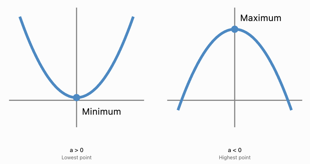
The vertex is the turning point of a parabola.
For an upward-opening parabola, the vertex is the lowest point.
For a downward-opening parabola, the vertex is the highest point.
The Coordinates of the Vertex
The vertex has coordinates:
(h, k)
where:
-
h is the input value that produces the optimum.
-
k is the maximum or minimum output.
Example
Consider:
P(x) = −2(x − 5)² + 100
The vertex is:
(5, 100)
If P represents profit, this means the maximum profit is 100 units when the input is 5.
Finding the Vertex from Standard Form
For:
y = ax² + bx + c
the x-coordinate of the vertex is:
x = −b/(2a)
Substitute this value into the equation to find the maximum or minimum output.
Worked Example
Find the maximum value of:
y = −2x² + 16x + 3
Step 1: Identify the Coefficients
a = −2
b = 16
c = 3
Step 2: Determine the Direction of Opening
Since a is negative, the parabola opens downward.
Therefore, the vertex is a maximum.
Step 3: Calculate the x-Coordinate
x = −16/[2(−2)]
x = −16/−4
x = 4
Step 4: Calculate the y-Coordinate
y = −2(4)² + 16(4) + 3
y = −32 + 64 + 3
y = 35
Final Answer
The maximum value is 35, occurring when x = 4.
The vertex is:
(4, 35)
Optimisation Using Vertex Form
Vertex form makes maximum and minimum values easier to identify.
y = a(x − h)² + k
The vertex is:
(h, k)
Example: Maximum
y = −3(x − 6)² + 80
The vertex is:
(6, 80)
The maximum value is:
80
This occurs when:
x = 6
Example: Minimum
y = 2(x + 4)² − 7
The vertex is:
(−4, −7)
The minimum value is:
−7
This occurs when:
x = −4
Important Observation
Vertex form is particularly useful in optimisation because the optimal input and output can be read directly from the equation.
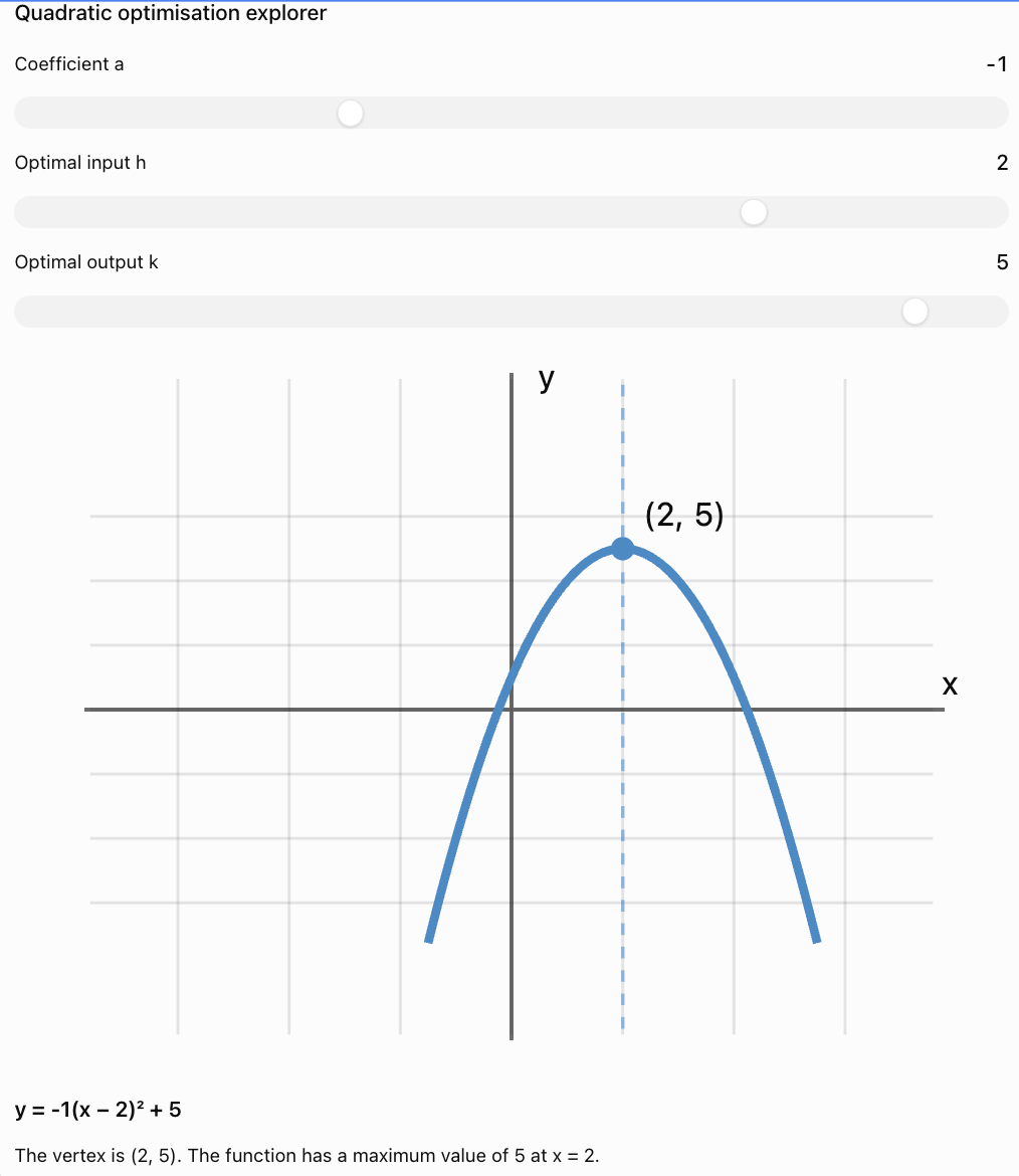
Exploring Maximum and Minimum Values
Change the coefficient and vertex position to investigate how the optimum changes.
Key Observation
The sign of a determines whether the vertex is a maximum or minimum.
The value h determines where the optimum occurs.
The value k determines the optimal output.
Optimising the Area of a Garden
One of the most common applications of quadratic optimisation is maximising area using a fixed amount of fencing.

Problem
A gardener has 40 metres of fencing to build a rectangular garden.
What dimensions will produce the largest possible area?
Step 1: Define Variables
Let:
w = width in metres
l = length in metres
A = area in square metres
Step 2: Write the Perimeter Equation
2w + 2l = 40
Divide by 2:
w + l = 20
Rearrange:
l = 20 − w
Step 3: Write the Area Equation
A = lw
Substitute:
A = w(20 − w)
Expand:
A(w) = −w² + 20w
Step 4: Find the Vertex
a = −1
b = 20
w = −20/[2(−1)]
w = 10 m
Step 5: Find the Length
l = 20 − 10
l = 10 m
Step 6: Calculate Maximum Area
A = 10 × 10
A = 100 m²
Final Answer
The maximum area is 100 m², achieved with a square garden measuring 10 m by 10 m.
Important Observation
When a rectangle has a fixed perimeter, the greatest area occurs when the rectangle is a square.
Optimising Area with Three Sides of Fencing
Sometimes a garden is built against a wall or river, so only three sides need fencing.
Problem
A farmer has 60 metres of fencing to enclose three sides of a rectangular field beside a straight wall.
Find the dimensions that maximise the area.
Step 1: Define Variables
Let:
w = width perpendicular to the wall
l = length parallel to the wall
Step 2: Write the Fencing Equation
2w + l = 60
Rearrange:
l = 60 − 2w
Step 3: Write the Area Equation
A = lw
A = w(60 − 2w)
A(w) = −2w² + 60w
Step 4: Find the Vertex
w = −60/[2(−2)]
w = 15 m
Step 5: Find the Length
l = 60 − 2(15)
l = 30 m
Step 6: Calculate the Maximum Area
A = 15 × 30
A = 450 m²
Final Answer
The maximum area is 450 m², with dimensions 15 m by 30 m.
Optimising Business Revenue
Businesses use optimisation to determine prices and quantities that produce the greatest revenue.
Problem
A company estimates that the selling price of a product is:
p = 80 − 2x
where:
-
p = price per item in dollars
-
x = number of items sold
Find the quantity that maximises revenue.
Step 1: Write the Revenue Equation
Revenue = price × quantity
R(x) = x(80 − 2x)
R(x) = −2x² + 80x
Step 2: Find the Vertex
a = −2
b = 80
x = −80/[2(−2)]
x = 20
Step 3: Calculate Maximum Revenue
R(20) = −2(20)² + 80(20)
R(20) = −800 + 1600
R(20) = $800
Step 4: Find the Selling Price
p = 80 − 2(20)
p = $40
Interpretation
The model predicts maximum revenue when the company sells 20 items at $40 each.
Important Distinction
Maximum revenue is not necessarily maximum profit.
Profit also depends on production and operating costs.
Optimising Business Profit
Profit is calculated using:
Profit = Revenue − Cost
Problem
A company's profit is modelled by:
P(x) = −3x² + 60x − 100
where x is the number of units produced, and P is measured in dollars.
Find the quantity that maximises profit.
Step 1: Identify Coefficients
a = −3
b = 60
c = −100
Step 2: Find the Optimal Quantity
x = −60/[2(−3)]
x = 10
Step 3: Calculate Maximum Profit
P(10) = −3(10)² + 60(10) − 100
P(10) = −300 + 600 − 100
P(10) = $200
Interpretation
The maximum predicted profit is $200 when 10 units are produced.
Important Observation
The vertex identifies the quantity that produces the greatest profit under the assumptions of the model.
Optimising Projectile Height
Projectile motion provides another important example of maximisation.

Problem
A ball is launched upward from ground level.
Its height is:
h(t) = −5t² + 30t
where:
-
h = height in metres
-
t = time in seconds
Find the maximum height.
Step 1: Identify Coefficients
a = −5
b = 30
Step 2: Find the Time at Maximum Height
t = −30/[2(−5)]
t = 3 seconds
Step 3: Calculate Maximum Height
h(3) = −5(3)² + 30(3)
h(3) = −45 + 90
h(3) = 45 m
Final Answer
The ball reaches a maximum height of 45 metres after 3 seconds.
Important Observation
The vertex provides both the optimal input and the maximum output.
Minimising Manufacturing Costs
Optimisation is also useful for reducing production costs.

Problem
A manufacturer's daily operating cost is modelled by:
C(x) = 2x² − 40x + 500
where x represents a production level in suitable units and C is measured in dollars.
Find the production level that minimises cost.
Step 1: Identify the Coefficients
a = 2
b = −40
c = 500
Step 2: Determine the Direction
Since a is positive, the parabola opens upward.
The vertex is a minimum.
Step 3: Find the Vertex
x = −(−40)/[2(2)]
x = 40/4
x = 10
Step 4: Calculate Minimum Cost
C(10) = 2(10)² − 40(10) + 500
C(10) = 200 − 400 + 500
C(10) = $300
Interpretation
According to the model, the minimum daily operating cost is $300 at a production level of 10 units.
Important Observation
The cost equation is a simplified model. Real manufacturing costs may not follow a quadratic relationship across all production levels.
Optimisation with Constraints
Real-world optimisation problems usually have restrictions.
These are called constraints.
Examples include:
-
A limited amount of fencing
-
A maximum budget
-
A minimum production quantity
-
A restricted amount of time
-
Available materials
-
Physical dimensions
Example
Suppose:
A(x) = −x² + 20x
The vertex occurs at:
x = 10
However, imagine the width must satisfy:
2 ≤ x ≤ 8
The vertex is outside the permitted domain.
Since the function is increasing throughout this interval, the maximum occurs at:
x = 8
Calculate:
A(8) = −8² + 20(8)
A(8) = −64 + 160
A(8) = 96
Important Observation
The vertex gives the optimum for an unrestricted quadratic function, but a restricted problem may have its optimum at a boundary.
Interpreting Optimal Solutions
Finding the vertex is only part of an optimisation problem.
The answer must also be interpreted.
Example
A revenue function has vertex:
(12.5, 312.5)
If x represents the number of products sold, then x = 12.5 is not a practical quantity.
We must compare nearby whole-number values.
For:
R(x) = −2x² + 50x
R(12) = $312
R(13) = $312
Interpretation
The best whole-number quantities are 12 or 13 items.
Both produce maximum revenue of $312.
Important Observation
An optimal mathematical answer may require adjustment to satisfy real-world restrictions.
Why Optimisation Is Useful
Optimisation is used in many areas of life.
Business and Economics
Companies use optimisation to:
-
Maximise profit
-
Minimise costs
-
Determine suitable prices
-
Allocate limited resources
Engineering
Engineers use optimisation to:
-
Reduce material usage
-
Improve structural designs
-
Minimise energy consumption
-
Improve efficiency
Agriculture
Farmers and gardeners use optimisation to:
-
Maximise planting area
-
Reduce fencing costs
-
Use available land efficiently
Sports and Physics
Optimisation can help analyse:
-
Maximum projectile height
-
Best launch conditions under specified constraints
-
Efficient movement and performance
Environmental Science
Optimisation may help:
-
Reduce waste
-
Improve resource allocation
-
Minimise energy use
-
Design efficient systems
A General Method for Solving Optimisation Problems
-
Understand the problem. Determine what must be maximised or minimised.
-
Define variables. Identify the independent and dependent quantities, including units.
-
Identify constraints. Determine any restrictions on the variables.
-
Create a quadratic model. Express the quantity to optimise as a function of one variable.
-
Find the vertex. Use vertex form or x = −b/(2a).
-
Check the domain. Compare the vertex with relevant endpoints or permitted integer values.
-
Interpret the result. Explain the optimal input and output in context.
-
Evaluate the model. Consider assumptions, accuracy, and whether the result is realistic.
Common Mistakes
Confusing the optimal input with the optimal output
The x-coordinate tells us where the optimum occurs. The y-coordinate tells us the maximum or minimum value.
Assuming every parabola has a maximum
Upward-opening parabolas have a minimum. Downward-opening parabolas have a maximum.
Forgetting to substitute the vertex x-coordinate
Finding x = −b/(2a) gives only the input. The output must also be calculated.
Ignoring constraints
A mathematically correct vertex may lie outside the permitted domain.
Using impossible dimensions
Lengths and widths must satisfy physical restrictions.
Confusing revenue and profit
Revenue is money received from sales. Profit is revenue minus costs.
Failing to define variables
Every variable should have a clear meaning and appropriate units.
Assuming decimal solutions are always practical
Whole-item quantities may require checking neighbouring integers.
Forgetting units
An area should be expressed in square units, not ordinary length units.
Assuming every real-world relationship is quadratic
Quadratic models are useful approximations in some situations but may not apply everywhere.
Key Terms
-
Optimisation: Finding the best possible solution under given conditions.
-
Maximisation: Finding the greatest possible value.
-
Minimisation: Finding the smallest possible value.
-
Optimal Solution: Best feasible value satisfying the constraints.
-
Objective Function: Function representing the quantity being maximised or minimised.
-
Constraint: Restriction on the values allowed in a problem.
-
Quadratic Function: Function whose highest variable power is two.
-
Parabola: Graph of a quadratic function.
-
Vertex: Maximum or minimum point of a parabola.
-
Maximum Value: Greatest output of a function over its domain.
-
Minimum Value: Smallest output of a function over its domain.
-
Vertex Form: Quadratic written as y = a(x − h)² + k.
-
Standard Form: Quadratic written as y = ax² + bx + c.
-
Axis of Symmetry: Vertical line passing through the vertex.
-
Independent Variable: Input variable.
-
Dependent Variable: Output variable.
-
Domain: Set of permitted input values.
-
Range: Set of possible output values.
-
Revenue: Total money received from sales.
-
Profit: Revenue minus costs.
-
Cost Function: Mathematical function describing expenses.
-
Area Function: Function describing how area depends on one or more dimensions.
-
Mathematical Model: Equation or representation describing a real-world situation.
-
Boundary Value: Value at an endpoint of a restricted domain.
-
Feasible Solution: Solution satisfying all constraints.
Key Takeaways
-
Optimisation involves finding maximum or minimum values.
-
Quadratic functions are useful for optimisation because their graphs have a single vertex.
-
An upward-opening parabola has a minimum.
-
A downward-opening parabola has a maximum.
-
The vertex gives the optimal input and output for an unrestricted quadratic function.
-
The vertex x-coordinate can be calculated using x = −b/(2a).
-
Vertex form makes maximum and minimum values easy to identify.
-
Practical optimisation problems require clearly defined variables.
-
Constraints must be considered before accepting a solution.
-
The optimum may occur at a boundary rather than at the vertex.
-
Mathematical solutions must be interpreted using appropriate units.
-
Optimisation is useful for maximising profit, revenue, area, and height.
-
Optimisation is also useful for minimising cost, waste, and resource consumption.
-
Real-world models should be evaluated for accuracy and realistic assumptions.
Check Your Understanding
Identifying Maximum and Minimum Values
-
What is optimisation?
-
What is the difference between maximisation and minimisation?
-
Does y = 3x² + 5 have a maximum or minimum?
-
Does y = −2x² + 8 have a maximum or minimum?
-
What point on a parabola represents the optimum?
Finding the Vertex
-
Find the vertex of y = −x² + 10x.
-
Determine the maximum value of the function in Question 6.
-
Find the minimum value of y = 2(x − 3)² + 4.
-
Find the vertex of y = x² − 8x + 10.
-
Explain why vertex form is useful for optimisation.
Practical Problems
-
A rectangular garden has perimeter 20 m. What dimensions maximise its area?
-
Find the maximum area of the garden in Question 11.
-
A revenue function is R(x) = −x² + 12x. Find the quantity that maximises revenue.
-
Find the maximum revenue in Question 13.
-
A projectile follows h(t) = −5t² + 20t. Find its maximum height.
Interpretation and Constraints
-
Why must constraints be considered in optimisation problems?
-
What is the difference between revenue and profit?
-
A quadratic model predicts an optimal production quantity of 8.5 items. What should be done?
-
Why might a mathematical optimum be unrealistic?
-
Give two real-world applications of optimisation.
Answer Key
|
Question |
Answer |
|---|---|
|
1 |
Finding the best possible value under given conditions |
|
2 |
Maximisation finds the greatest value; minimisation finds the smallest |
|
3 |
Minimum |
|
4 |
Maximum |
|
5 |
Vertex |
|
6 |
(5, 25) |
|
7 |
25 |
|
8 |
4 |
|
9 |
(4, −6) |
|
10 |
The optimal input and output can be read directly |
|
11 |
5 m by 5 m |
|
12 |
25 m² |
|
13 |
x = 6 |
|
14 |
36 |
|
15 |
20 m |
|
16 |
They restrict the feasible solutions |
|
17 |
Profit equals revenue minus costs |
|
18 |
Compare feasible whole-number quantities, such as 8 and 9 |
|
19 |
It may violate constraints or model assumptions |
|
20 |
Garden design, business profit, manufacturing costs, or projectile height |
Extended Challenge
-
Find the maximum value of y = −3x² + 24x − 10.
-
Find the minimum value of y = 4x² − 32x + 70.
-
A rectangle has perimeter 50 m. Determine the dimensions that maximise its area.
-
Find the maximum area of the rectangle in Question 3.
-
A farmer has 80 m of fencing for three sides of a rectangular field beside a river. Determine the optimal dimensions.
-
Find the maximum area of the field in Question 5.
-
A revenue model is R(x) = −4x² + 100x. Find the quantity that maximises revenue.
-
Determine the maximum revenue in Question 7 when only whole items can be sold.
-
A manufacturing cost model is C(x) = 3x² − 36x + 200. Find the minimum cost.
-
A projectile follows h(t) = −5t² + 40t + 2. Find its maximum height and the time at which it occurs.
Final Investigation: Designing an Optimal Garden
A school has 60 metres of fencing to construct a rectangular garden.
The school wants to maximise the planting area while using all the fencing.
Investigation Tasks
-
Define the width and length variables.
-
Write the perimeter equation.
-
Rearrange the equation to express length in terms of width.
-
Write the area equation.
-
Expand the area equation into standard quadratic form.
-
Identify the coefficients a, b, and c.
-
Explain why the graph opens downward.
-
Determine the vertex.
-
Interpret the vertex in the context of the garden.
-
Calculate the maximum area.
-
Determine the dimensions that produce the maximum area.
-
Create a table of values for several possible widths.
-
Graph the area function.
-
Identify the axis of symmetry.
-
Determine the physically meaningful domain.
-
Explain why negative widths are not acceptable.
-
Explain why a width greater than 30 m is impossible.
-
Compare the areas of gardens measuring 10 m by 20 m and 15 m by 15 m.
-
Explain why the optimal garden is a square.
-
Write a conclusion explaining how quadratic optimisation helps make efficient use of limited resources.
Investigation Check
The area equation is:
A(w) = −w² + 30w
The vertex is:
(15, 225)
Therefore:
-
Optimal width: 15 m
-
Optimal length: 15 m
-
Maximum area: 225 m²
The physically meaningful domain is:
0 < w < 30
4. Quadratic Modelling with Technology
Learning outcomes
- I can use graphing technology to model data.
- I can interpret quadratic regression results.
- I can compare a model with real data.
- I can identify limitations of a quadratic model.
- I can make predictions using a quadratic model.
Quadratic Modelling with Technology
Introduction
Mathematical models help us identify patterns, describe relationships, and make predictions from real-world data.
When data follows a curved pattern, a quadratic function may provide a useful model. Graphing technology allows us to analyse these relationships more efficiently than performing every calculation by hand.
Tools such as graphing calculators, spreadsheets, Desmos, and GeoGebra can help us:
-
Organise and graph measured data.
-
Identify patterns in scatter plots.
-
Calculate quadratic regression equations.
-
Compare predicted values with actual observations.
-
Find maximum and minimum values.
-
Evaluate the accuracy and limitations of a model.
-
Make predictions about future or unknown values.
Quadratic modelling is especially useful in physics, engineering, economics, environmental science, and other fields where quantities change at a nonconstant rate.


What Is Mathematical Modelling?
A mathematical model is an equation, graph, table, or other mathematical representation used to describe a real-world relationship.
For example, a model might describe:
-
The height of a projectile over time.
-
The relationship between a vehicle's speed and braking distance.
-
The area of a garden as its dimensions change.
-
The revenue earned by a business at different selling prices.
-
The relationship between production quantity and manufacturing costs.
A model simplifies a situation so that mathematical methods can be used to analyse it.
Important Observation
A mathematical model is not necessarily an exact description of reality. It is a representation based on available data and assumptions.
Recognising Quadratic Relationships in Data
A quadratic function has the general form:
y = ax² + bx + c
where a ≠ 0.
Its graph is a parabola.
Quadratic relationships often appear when:
-
Data increases and then decreases.
-
Data decreases and then increases.
-
A quantity has a maximum or minimum.
-
The rate of change varies in a roughly linear way.
-
A relationship involves the square of a variable.
Example
A ball is launched upward, and its height is measured at different times.
|
Time (s) |
Height (m) |
|---|---|
|
0 |
0 |
|
1 |
15 |
|
2 |
20 |
|
3 |
15 |
|
4 |
0 |
The height increases, reaches a maximum, and then decreases.
This pattern suggests a downward-opening parabola.
A quadratic function is therefore a reasonable model to investigate.
Using Scatter Plots
A scatter plot displays pairs of numerical data as points on a coordinate plane.
Each point represents one observation.
For example:
(0, 0)
(1, 15)
(2, 20)
(3, 15)
(4, 0)
Why Use a Scatter Plot?
Scatter plots help us:
-
Identify curved or linear patterns.
-
Detect unusual measurements.
-
Observe possible maximum and minimum values.
-
Compare measured data with a mathematical model.
-
Decide which type of regression may be appropriate.
Important Observation
A scatter plot displays actual observations. A regression curve represents a mathematical model fitted to those observations.
The curve does not necessarily pass through every point.
Quadratic Regression
Quadratic regression is a statistical technique used to find a quadratic equation that best fits a set of data.
The model has the form:
ŷ = ax² + bx + c
The symbol ŷ represents a predicted value.
Graphing technology calculates values for a, b, and c that make the model fit the observations as closely as possible according to a selected fitting method.
Most standard quadratic regression tools use least squares regression.
This method minimises the sum of the squared vertical differences between observed and predicted values.
Example
Suppose graphing technology produces:
ŷ = −4.8x² + 19.5x + 1.2
This could represent the height of a projectile.
The coefficients have mathematical meanings:
-
a = −4.8 controls the curvature and indicates a downward-opening parabola.
-
b = 19.5 represents the initial rate of change in the model.
-
c = 1.2 represents the predicted height when x = 0.
Important Observation
Regression finds a model from data. The coefficients are estimates and may differ slightly from the values expected from a theoretical equation.
How Least Squares Regression Works
Suppose a quadratic model predicts a height of 12 metres, but the measured height is 11.5 metres.
The difference is called a residual.
Residual = observed value − predicted value
Residual = 11.5 − 12
Residual = −0.5 m
The squared residual is:
(−0.5)² = 0.25
For a set of observations, least squares regression chooses the coefficients that minimise:
SSE = Σ(observed − predicted)²
where SSE means sum of squared errors.
Why Square the Residuals?
Squaring:
-
Prevents positive and negative residuals from cancelling.
-
Gives larger errors greater influence.
-
Produces a mathematical quantity that can be minimised.
Important Observation
A regression equation is generally an approximation, not a perfect equation through all measured points.
Creating a Quadratic Regression Model
Consider the following experimental data.
|
Time (s) |
Measured height (m) |
|---|---|
|
0 |
1.0 |
|
1 |
15.8 |
|
2 |
20.9 |
|
3 |
16.1 |
|
4 |
1.2 |
The values suggest that the object rises and then falls.
A suitable approximate model is:
h(t) = −5t² + 20t + 1
Comparing the Model with Observations
|
Time (s) |
Observed height (m) |
Predicted height (m) |
Residual (m) |
|---|---|---|---|
|
0 |
1.0 |
1 |
0.0 |
|
1 |
15.8 |
16 |
−0.2 |
|
2 |
20.9 |
21 |
−0.1 |
|
3 |
16.1 |
16 |
0.1 |
|
4 |
1.2 |
1 |
0.2 |
This equation is a simple illustrative model, not the exact least-squares regression result.
The differences between observed and predicted heights are small, suggesting that the model describes these measurements reasonably well.
Exploring the Fit of a Quadratic Model
The following graph shows the measured data and the illustrative quadratic model.
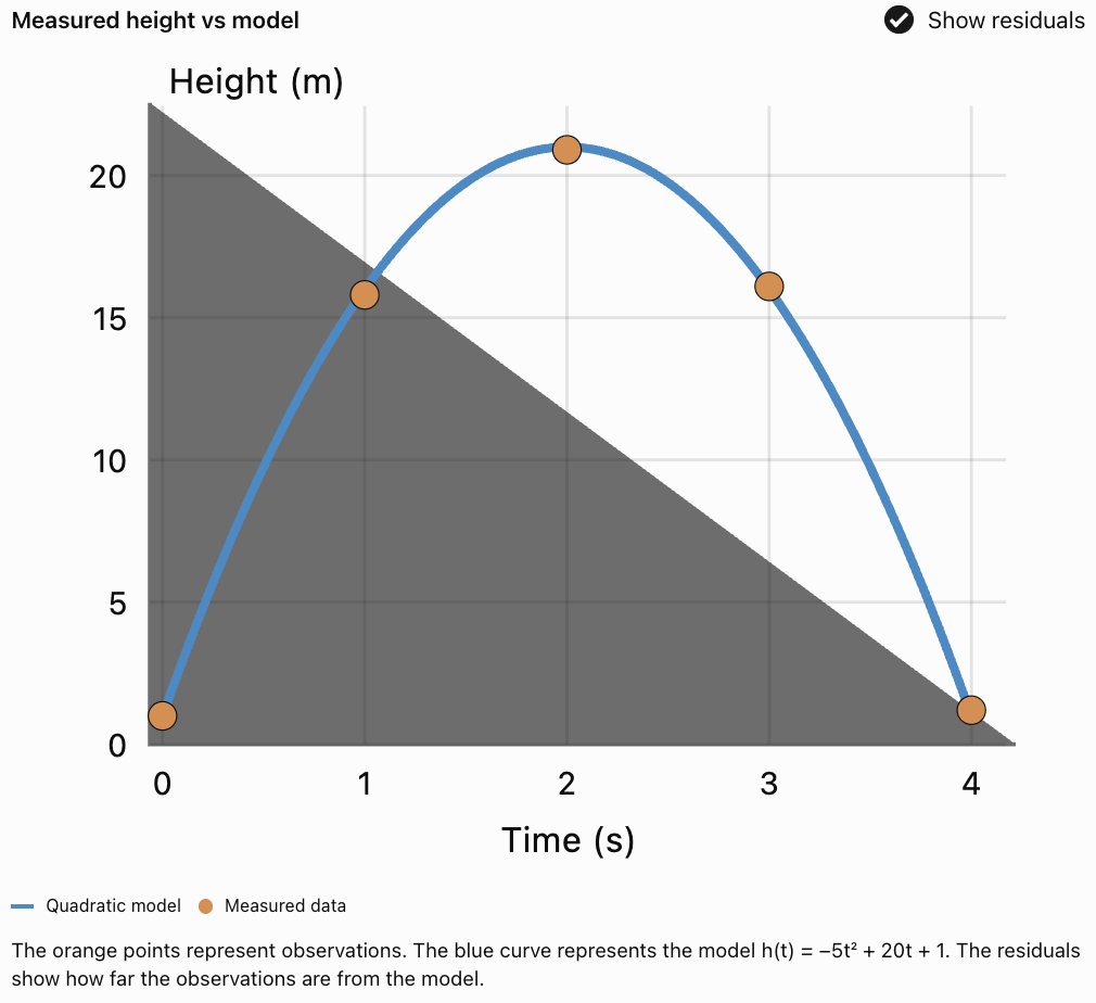
Interpretation
Most measured points lie close to the curve.
This suggests that a quadratic model is appropriate for the observed time interval.
However, a close fit does not guarantee that the model will remain accurate outside that interval.
Using Desmos for Quadratic Regression
Open Desmos Graphing Calculator
Desmos provides a convenient way to create scatter plots and perform regression.
Procedure
-
Open the Desmos Graphing Calculator.
-
Select Add Item, then Table.
-
Enter the independent-variable values in the first column.
-
Enter the dependent-variable values in the second column.
-
Create a new expression using the table column names.
For a standard table named x₁ and y₁, enter:
y₁ ~ ax₁² + bx₁ + c
The tilde symbol (~) tells Desmos to perform regression.
Desmos calculates values for a, b, and c.
What to Examine
After calculating the regression:
-
Record the equation.
-
Examine the shape of the fitted curve.
-
Identify the vertex.
-
Compare the curve with the observed points.
-
Examine the residuals.
-
Decide whether the model makes sense in context.
Important Observation
In Desmos, the regression expression uses ~ rather than = because the software is estimating coefficients from measured data.
Using GeoGebra for Quadratic Regression
Open GeoGebra Graphing Calculator
GeoGebra can also be used to analyse quadratic relationships.
General Procedure
-
Enter the observed data as points.
-
Display the points on the coordinate plane.
-
Create a list of the points.
-
Use a quadratic polynomial fitting command such as
FitPoly(list, 2), with the actual point-list name substituted forlist. -
Display the resulting quadratic equation.
-
Compare the fitted curve with the observed points.
Important Observation
Different graphing tools may display equations or coefficients with slightly different rounding.
When the same data and least-squares method are used, the underlying results should be consistent.
Using Spreadsheets for Quadratic Modelling
Spreadsheet programs such as Excel and Google Sheets can also perform quadratic regression.

General Procedure
-
Enter x-values in one column.
-
Enter y-values in another column.
-
Create an XY scatter chart.
-
Add a trendline.
-
Select a polynomial trendline.
-
Set the polynomial order to 2.
-
Display the equation and R² value if the software supports these options.
Important Observation
A polynomial trendline of order 2 represents a quadratic function.
An order-1 polynomial represents a linear function.
Interpreting Regression Coefficients
Suppose the regression equation is:
ŷ = −2.5x² + 15x + 8
Coefficient a
a = −2.5
The parabola opens downward.
The model has a maximum.
Coefficient b
b = 15
This affects the position of the vertex and the rate of change.
In a model where x represents time, it may represent an initial rate of change.
Coefficient c
c = 8
The predicted value when x = 0 is 8.
Finding the Vertex
x = −b/(2a)
x = −15/[2(−2.5)]
x = 3
Substitute:
ŷ = −2.5(3)² + 15(3) + 8
ŷ = −22.5 + 45 + 8
ŷ = 30.5
Interpretation
The model predicts a maximum value of 30.5 when x = 3.
The real-world meaning depends on the variables and units.
Understanding the Coefficient of Determination
Graphing technology may report a value called R², known as the coefficient of determination.
For ordinary regression with an intercept, it is commonly calculated as:
R² = 1 − SSE/SST
where:
-
SSE = sum of squared residuals.
-
SST = sum of squared differences between observed values and their mean.
Interpreting R²
|
R² value |
General interpretation |
|---|---|
|
1.00 |
Perfect fit to the observed data |
|
0.95 |
Very strong fit to the observed data |
|
0.80 |
Substantial variation explained |
|
0.50 |
Moderate explanatory fit |
|
Near 0 |
Little improvement over predicting the mean |
These are illustrative interpretations, not universal thresholds. Whether a fit is acceptable depends on the subject, measurement accuracy, and purpose of the model.
Example
Suppose:
R² = 0.96
This indicates that approximately 96% of the variation in the observed dependent variable is accounted for by the fitted model, using the usual R² definition.
Important Observation
A high R² does not prove that a model is correct, that the relationship is causal, or that future predictions will be accurate.
Comparing Predicted and Observed Values
After creating a regression equation, compare its predictions with actual measurements.
Example
Suppose a model predicts:
ŷ = 2x² + 3x + 1
At x = 2:
ŷ = 2(2)² + 3(2) + 1
ŷ = 8 + 6 + 1
ŷ = 15
If the observed value is 14.5:
Residual = 14.5 − 15
Residual = −0.5
Interpretation
The model overestimated the observation by 0.5 units.
A table of residuals can help determine whether the model consistently overestimates or underestimates particular regions of the data.
Residual Plots
A residual plot displays residuals against the independent variable.
Residual plots are useful for detecting patterns that may not be obvious from the original scatter plot.
A Suitable Model
If residuals are scattered approximately randomly around zero, the model may describe the data reasonably well.
An Unsuitable Model
If residuals form a systematic curve or trend, the chosen model may be missing an important pattern.
Other Warning Signs
-
Residuals become larger as x increases.
-
One or two points have unusually large residuals.
-
Residuals remain mostly positive or mostly negative over a long interval.
Important Observation
A residual plot can reveal problems even when the original regression curve appears to fit the data well.
Making Predictions Using a Quadratic Model
Once a suitable model has been developed, it can be used to estimate values that were not directly measured.
Worked Example
Suppose a quadratic regression model for a projectile is:
h(t) = −4.9t² + 19.6t + 1.5
where:
-
t = time in seconds
-
h = height in metres
Find the predicted height after 1.5 seconds.
Step 1: Substitute the Time
h(1.5) = −4.9(1.5)² + 19.6(1.5) + 1.5
Step 2: Calculate
h(1.5) = −4.9(2.25) + 29.4 + 1.5
h(1.5) = −11.025 + 29.4 + 1.5
h(1.5) = 19.875 m
Interpretation
The model predicts a height of approximately 19.9 metres after 1.5 seconds.
This is a prediction, not necessarily an exact measured height.
Predicting Maximum and Minimum Values
A quadratic regression equation can also be used to estimate maximum or minimum values.
For:
y = ax² + bx + c
the x-coordinate of the vertex is:
x = −b/(2a)
Example
A company's profit is modelled by:
P(x) = −2x² + 48x − 100
where x represents the number of products sold and P is measured in dollars.
Find the Optimal Quantity
x = −48/[2(−2)]
x = 12
Find the Maximum Profit
P(12) = −2(12)² + 48(12) − 100
P(12) = −288 + 576 − 100
P(12) = $188
Interpretation
The model predicts a maximum profit of $188 when 12 products are sold.
Important Observation
The vertex gives the optimum of the quadratic equation, but the answer must still satisfy the practical constraints of the situation.
Interpolation and Extrapolation
Predictions can be classified into two categories.
Interpolation
Interpolation involves predicting a value within the range of observed data.
Suppose measurements were collected for:
0 ≤ t ≤ 5 seconds
Predicting the value at t = 2.5 seconds is interpolation.
This is generally more reliable because the prediction lies within the measured interval.
Extrapolation
Extrapolation involves predicting a value outside the observed data range.
Using the same measurements to predict the value at t = 15 seconds is extrapolation.
This is generally less reliable because the relationship may change beyond the measured interval.
Example
A projectile model may predict a negative height long after the projectile has landed.
Although the equation can be evaluated mathematically, the result does not describe the object's actual position after impact.
Important Conclusion
A model should only be used for predictions within a range where its assumptions and behaviour remain reasonable.
Comparing Linear and Quadratic Regression
Graphing technology allows us to compare different models fitted to the same data.
Consider:
|
x |
y |
|---|---|
|
0 |
2 |
|
1 |
4 |
|
2 |
8 |
|
3 |
14 |
|
4 |
22 |
First Differences
2, 4, 6, 8
These are not constant.
Second Differences
2, 2, 2
These are constant.
The data follow an exact quadratic pattern.
A suitable equation is:
y = x² + x + 2
Comparing Models
A linear regression model would produce a straight line that does not pass through all five points.
The quadratic model passes through every point.
Important Observation
A quadratic model may fit curved data better than a linear model, but greater complexity is not always desirable. Models should be selected based on accuracy, simplicity, physical reasoning, and their ability to predict new observations.
Limitations of Quadratic Regression
Quadratic regression is powerful, but it has limitations.
Measurement Error
Real-world measurements may contain errors caused by instruments, human observation, or environmental conditions.
Limited Data
A model based on only a few measurements may not reliably represent the full relationship.
In particular, three distinct x-values can determine an exact quadratic equation even if the data do not come from a genuinely quadratic process.
Outliers
An unusually high or low observation can influence the fitted curve.
Incorrect Model Type
Some relationships are exponential, logarithmic, periodic, or more complicated than a quadratic function.
Restricted Domains
A model may only apply over a particular range of inputs.
Changing Conditions
Real-world conditions may change after data collection.
For example, production costs, weather conditions, or physical forces may vary.
Correlation Does Not Establish Causation
A quadratic relationship between two variables does not automatically mean that one variable causes changes in the other.
Evaluating the Quality of a Model
A useful quadratic model should satisfy several criteria.
|
Criterion |
Question to consider |
|---|---|
|
Visual fit |
Does the curve follow the overall pattern of the data? |
|
Residuals |
Are errors reasonably small and free of obvious patterns? |
|
R² |
How much observed variation does the model account for? |
|
Physical meaning |
Does the equation make sense in context? |
|
Domain |
Are predictions restricted to meaningful inputs? |
|
Assumptions |
Are the simplifying assumptions reasonable? |
|
Prediction accuracy |
Does the model predict new observations successfully? |
Important Observation
No single statistic is sufficient to determine whether a model is appropriate.
A strong evaluation considers both mathematical accuracy and real-world meaning.
Improving a Quadratic Model
If a model does not fit the observations well, several improvements may be possible.
-
Collect more measurements across the relevant input range.
-
Check for recording or measurement errors.
-
Investigate unusually large residuals.
-
Use more precise measuring instruments.
-
Compare quadratic regression with other model types.
-
Restrict the model to a range where the relationship is valid.
-
Test predictions against new observations.
Example
Suppose a quadratic model describes the first five seconds of a ball's motion accurately but becomes unrealistic after the ball lands.
Rather than extending the same equation indefinitely, restrict the model to the time interval during which the ball is actually in flight.
Real-World Applications of Quadratic Regression
Physics
Experimental height-time data can be used to estimate projectile motion.

Transportation
Vehicle-speed and braking-distance measurements can be analysed using quadratic models.
Business
Sales and revenue data can be used to estimate optimal production quantities or prices.
Engineering
Measured points on curved structures can be used to fit parabolic models.
Agriculture
Data relating planting dimensions to area or production can be analysed to identify useful mathematical relationships.
Important Observation
The value of quadratic regression comes from combining mathematical techniques with meaningful data and appropriate interpretation.
Common Mistakes
Assuming regression produces an exact equation
Regression usually produces an approximation based on measured data.
Confusing observed and predicted values
Observed values come from measurements. Predicted values come from the model.
Ignoring residuals
A curve may appear accurate while still producing systematic prediction errors.
Assuming R² = 1 proves a model is physically correct
A perfect fit to existing observations does not guarantee a correct underlying explanation.
Choosing quadratic regression for every curved pattern
Not all nonlinear relationships are quadratic.
Extrapolating too far
Predictions outside the observed range may be unreliable.
Ignoring units
Every coefficient and prediction must be interpreted in the context of the variables.
Rounding coefficients too early
Premature rounding can introduce errors into calculated predictions.
Ignoring outliers
Unusual measurements may significantly influence the regression equation.
Using unrealistic input values
A model may produce mathematically valid outputs that are impossible in the real situation.
Key Terms
-
Mathematical Model: Mathematical representation of a real-world relationship.
-
Quadratic Model: Model expressed using a quadratic function.
-
Quadratic Regression: Statistical method for fitting a quadratic equation to data.
-
Scatter Plot: Graph displaying paired numerical observations.
-
Regression Curve: Curve fitted to observed data.
-
Least Squares: Method that minimises the sum of squared residuals.
-
Observed Value: Value obtained from actual measurement.
-
Predicted Value: Value calculated using a mathematical model.
-
Residual: Difference between an observed and predicted value.
-
Sum of Squared Errors (SSE): Sum of squared residuals.
-
Coefficient of Determination (R²): Statistic describing the proportion of observed variation accounted for by a fitted model under the usual definition.
-
Residual Plot: Graph showing residuals against input values or predictions.
-
Outlier: Observation unusually far from the overall pattern.
-
Interpolation: Prediction within the observed data range.
-
Extrapolation: Prediction outside the observed data range.
-
Independent Variable: Input variable.
-
Dependent Variable: Output variable.
-
Vertex: Maximum or minimum point of a parabola.
-
Domain: Set of permitted input values.
-
Range: Set of possible output values.
-
Trendline: Line or curve fitted to data to represent a pattern.
-
Polynomial Regression: Regression using a polynomial function.
-
Measurement Error: Difference between a measurement and the actual quantity.
-
Model Limitation: Condition restricting the accuracy or usefulness of a model.
Key Takeaways
-
Graphing technology makes it easier to analyse real-world numerical data.
-
Scatter plots help identify relationships between variables.
-
Quadratic regression fits a parabola to measured data.
-
A quadratic regression equation has the form ŷ = ax² + bx + c.
-
The coefficients describe the shape and position of the fitted parabola.
-
Least squares regression minimises the sum of squared residuals.
-
Residuals measure differences between observed and predicted values.
-
Residual plots help identify patterns that a model may fail to explain.
-
R² provides information about how closely a model fits the observed data.
-
A high R² does not guarantee that the model is correct.
-
The vertex can be used to estimate maximum or minimum values.
-
Quadratic models can be used for interpolation and extrapolation.
-
Extrapolation is generally less reliable.
-
A model should be evaluated using mathematical accuracy, physical meaning, and appropriate assumptions.
-
Technology supports mathematical reasoning but does not replace interpretation.
Check Your Understanding
Understanding Quadratic Regression
-
What is quadratic regression?
-
What is the purpose of a scatter plot?
-
What does the symbol ŷ represent?
-
Why does least squares regression square the residuals?
-
What does a negative coefficient a indicate about the fitted parabola?
Interpreting Regression Results
-
A regression equation is ŷ = −2x² + 12x + 5. What is the predicted value when x = 0?
-
Determine the vertex of the equation in Question 6.
-
Does the equation have a maximum or minimum?
-
What does R² measure?
-
Does a high R² prove that a quadratic model is correct?
Comparing Models with Data
-
Define a residual.
-
Calculate the residual when the observed value is 18 and the predicted value is 20.
-
What does a positive residual indicate?
-
Why are residual plots useful?
-
What might a systematic curved pattern in residuals suggest?
Predictions and Limitations
-
Explain the difference between interpolation and extrapolation.
-
Why is extrapolation generally less reliable?
-
Give one reason a quadratic model might produce unrealistic predictions.
-
Why should units be included when interpreting regression results?
-
Name two technologies that can perform quadratic regression.
Answer Key
|
Question |
Answer |
|---|---|
|
1 |
Fitting a quadratic equation to numerical data |
|
2 |
To display relationships and patterns between two variables |
|
3 |
A predicted output |
|
4 |
To prevent cancellation and penalise larger errors |
|
5 |
The parabola opens downward |
|
6 |
5 |
|
7 |
(3, 23) |
|
8 |
Maximum |
|
9 |
The proportion of observed variation accounted for by the fitted model, under the usual definition |
|
10 |
No |
|
11 |
Observed value minus predicted value |
|
12 |
−2 |
|
13 |
The observed value is greater than the predicted value |
|
14 |
They help reveal systematic prediction errors |
|
15 |
The model may be missing an important pattern |
|
16 |
Interpolation is within the observed range; extrapolation is outside it |
|
17 |
Conditions and relationships may change outside the measured range |
|
18 |
Incorrect assumptions, limited domain, or an unsuitable model |
|
19 |
Units give physical meaning to values and predictions |
|
20 |
Desmos, GeoGebra, Excel, or Google Sheets |
Extended Challenge
-
A regression equation is ŷ = −3x² + 24x + 10. Determine the vertex.
-
Interpret the maximum value if y represents height in metres and x represents time in seconds.
-
Use the model in Question 1 to predict the height at x = 2.
-
Find the positive x-intercept of the model in Question 1.
-
A quadratic model predicts 35.2, but the observed value is 34.7. Calculate the residual.
-
Explain why a model with R² = 0.98 might still be inappropriate for long-term predictions.
-
Construct a quadratic equation through the points (0, 2), (1, 5), and (2, 10).
-
Explain why fitting exactly three points is not sufficient evidence that the real-world relationship is quadratic.
-
Compare the advantages of quadratic regression and manually fitting a parabola.
-
Describe how you would evaluate whether a quadratic model is more appropriate than a linear model for an experimental dataset.
Final Investigation: Modelling Projectile Data with Technology
A student records the height of a ball at different times during a projectile experiment.
The following measurements are collected:
|
Time (s) |
Height (m) |
|---|---|
|
0.0 |
1.2 |
|
0.5 |
8.4 |
|
1.0 |
13.2 |
|
1.5 |
15.6 |
|
2.0 |
16.1 |
|
2.5 |
13.5 |
|
3.0 |
8.9 |
|
3.5 |
1.5 |
Investigation Tasks
-
Identify the independent variable.
-
Identify the dependent variable.
-
Enter the data into Desmos, GeoGebra, or a spreadsheet.
-
Create a scatter plot.
-
Describe the pattern of the observations.
-
Explain why quadratic regression may be appropriate.
-
Calculate the quadratic regression equation using technology.
-
Record the coefficients a, b, and c.
-
Explain what the sign of a indicates.
-
Graph the regression curve alongside the measured points.
-
Record the R² value if available.
-
Calculate the predicted height at t = 1 second.
-
Calculate the predicted height at t = 2 seconds.
-
Find the residuals for the measurements at t = 1 and t = 2.
-
Create a residual plot.
-
Determine the predicted time at maximum height.
-
Calculate the predicted maximum height.
-
Estimate when the ball reaches ground level.
-
Identify two limitations of the model.
-
Write a conclusion evaluating how effectively quadratic regression describes the experimental data.
Investigation Guidance
A successful investigation should include:
-
A labelled scatter plot.
-
A quadratic regression equation.
-
A graph of the fitted parabola.
-
Calculated predictions and residuals.
-
The estimated vertex.
-
An explanation of the model's accuracy.
-
A discussion of assumptions and limitations.
Extension
Use the fitted equation to predict the ball's height at t = 5 seconds.
Explain whether the prediction is physically meaningful and whether it should be trusted.
Consider whether the ball would already have reached the ground.
5. Review and Problem Solving
Learning outcomes
- I can solve multi-step quadratic problems.
- I can choose appropriate mathematical methods.
- I can interpret solutions in context.
- I can communicate mathematical reasoning clearly.
- I can evaluate the reasonableness of my answers.
Review and Problem Solving: Quadratic Functions
Introduction
Quadratic functions are useful mathematical tools for solving problems involving patterns, graphs, equations, maximum and minimum values, and real-world situations.
In earlier topics, we explored how to recognise, graph, transform, and model quadratic functions. We also investigated projectile motion, optimisation, and quadratic regression.
This review brings these ideas together, focusing on multi-step problem solving.
Successful problem solving requires more than obtaining a numerical answer. It involves choosing an appropriate method, explaining the mathematical reasoning, interpreting results, and checking whether the answer is reasonable.


Reviewing Quadratic Functions
A quadratic function is a function that can be written as:
y = ax² + bx + c
where a, b, and c are constants and a ≠ 0.
The graph of a quadratic function is a parabola.
Important Characteristics
-
A positive a-value produces an upward-opening parabola.
-
A negative a-value produces a downward-opening parabola.
-
The vertex represents the maximum or minimum.
-
The axis of symmetry passes through the vertex.
-
A quadratic function can have zero, one, or two distinct real x-intercepts.
-
Quadratic functions can model many practical situations.
Example
Consider:
y = −2x² + 8x + 3
Since a = −2, the parabola opens downward.
Therefore, the function has a maximum value.
The Three Forms of Quadratic Functions
Quadratic functions can be expressed in three commonly used forms.
|
Form |
Equation |
Main advantage |
|---|---|---|
|
Standard |
y = ax² + bx + c |
Useful for identifying coefficients and applying the quadratic formula |
|
Vertex |
y = a(x − h)² + k |
Reveals the vertex and transformations |
|
Factored |
y = a(x − r₁)(x − r₂) |
Reveals the roots |
Example
Consider the function:
y = x² − 6x + 8
Standard form:
y = x² − 6x + 8
Factored form:
y = (x − 2)(x − 4)
Vertex form:
y = (x − 3)² − 1
All three equations represent the same parabola.
Important Observation
Choosing the most useful form can make a multi-step problem much easier.
Choosing the Appropriate Mathematical Method
Different quadratic problems require different approaches.
|
Problem |
Useful method |
|---|---|
|
Find x-intercepts |
Factoring, square roots, or quadratic formula |
|
Find the vertex |
Vertex form or x = −b/(2a) |
|
Identify transformations |
Vertex form |
|
Find a maximum or minimum |
Vertex |
|
Solve an equation that factors easily |
Factoring |
|
Solve an equation that does not factor easily |
Quadratic formula |
|
Determine the number of real roots |
Discriminant |
|
Model measured data |
Quadratic regression |
|
Interpret a real-world solution |
Apply context and domain restrictions |
Important Observation
A strong problem solver does not automatically use the same method for every problem.
The method should be selected based on the equation and what the question asks.
Solving Quadratic Equations by Factoring
Factoring is often the simplest method when a quadratic expression can be written as a product.
Worked Example
Solve:
x² − 7x + 12 = 0
Step 1: Find Two Numbers
We need two numbers that:
-
Multiply to 12.
-
Add to −7.
The numbers are −3 and −4.
Step 2: Factor
(x − 3)(x − 4) = 0
Step 3: Apply the Zero Product Property
x − 3 = 0
or
x − 4 = 0
Solutions
x = 3 or x = 4
Checking
For x = 3:
3² − 7(3) + 12 = 9 − 21 + 12 = 0
For x = 4:
4² − 7(4) + 12 = 16 − 28 + 12 = 0
Both solutions are correct.
Solving Quadratic Equations Using Square Roots
Square roots are particularly useful when the squared expression is isolated.
Worked Example
Solve:
3(x − 2)² = 27
Divide by 3:
(x − 2)² = 9
Take square roots:
x − 2 = ±3
Therefore:
x = 2 + 3
or
x = 2 − 3
Solutions
x = 5 or x = −1
Important Observation
Remember the positive and negative square roots when solving equations of this form.
Solving Using the Quadratic Formula
The quadratic formula can solve any quadratic equation written in standard form.
x = [−b ± √(b² − 4ac)]/(2a)
Worked Example
Solve:
2x² + 3x − 4 = 0
Identify:
a = 2
b = 3
c = −4
Substitute:
x = [−3 ± √(3² − 4(2)(−4))]/[2(2)]
x = [−3 ± √(9 + 32)]/4
x = [−3 ± √41]/4
Solutions
x = (−3 + √41)/4 ≈ 0.851
x = (−3 − √41)/4 ≈ −2.351
Important Observation
The quadratic formula is especially useful when factoring is difficult or impossible using simple integers.
Using the Discriminant
The discriminant is the expression:
D = b² − 4ac
It tells us how many distinct real solutions a quadratic equation has.
|
Discriminant |
Number of distinct real solutions |
|---|---|
|
D > 0 |
Two |
|
D = 0 |
One repeated root |
|
D < 0 |
None |
Worked Example
Determine the number of real solutions of:
x² − 4x + 7 = 0
a = 1
b = −4
c = 7
D = (−4)² − 4(1)(7)
D = 16 − 28
D = −12
Since the discriminant is negative, there are no real solutions.
Important Observation
The discriminant allows us to predict the number of real roots without calculating the roots themselves.
Finding the Vertex
The vertex is the turning point of a parabola.
For:
y = ax² + bx + c
the x-coordinate of the vertex is:
x = −b/(2a)
Worked Example
Find the vertex of:
y = −x² + 10x − 16
Step 1: Identify Coefficients
a = −1
b = 10
c = −16
Step 2: Find the x-Coordinate
x = −10/[2(−1)]
x = 5
Step 3: Find the y-Coordinate
y = −(5)² + 10(5) − 16
y = −25 + 50 − 16
y = 9
Final Answer
The vertex is:
(5, 9)
The maximum value is 9.
The axis of symmetry is x = 5.
Combining Transformations
Consider:
y = −2(x − 3)² + 4
Compared with the parent function y = x², the graph has undergone:
-
A horizontal translation 3 units right.
-
A vertical stretch by a factor of 2.
-
A reflection across the x-axis.
-
A vertical translation 4 units up.
Characteristics
-
Vertex: (3, 4)
-
Axis of symmetry: x = 3
-
Opens downward
-
Maximum value: 4
-
Range: y ≤ 4
Important Observation
Vertex form allows us to predict the graph before plotting points.
Visualising the Main Graph Characteristics
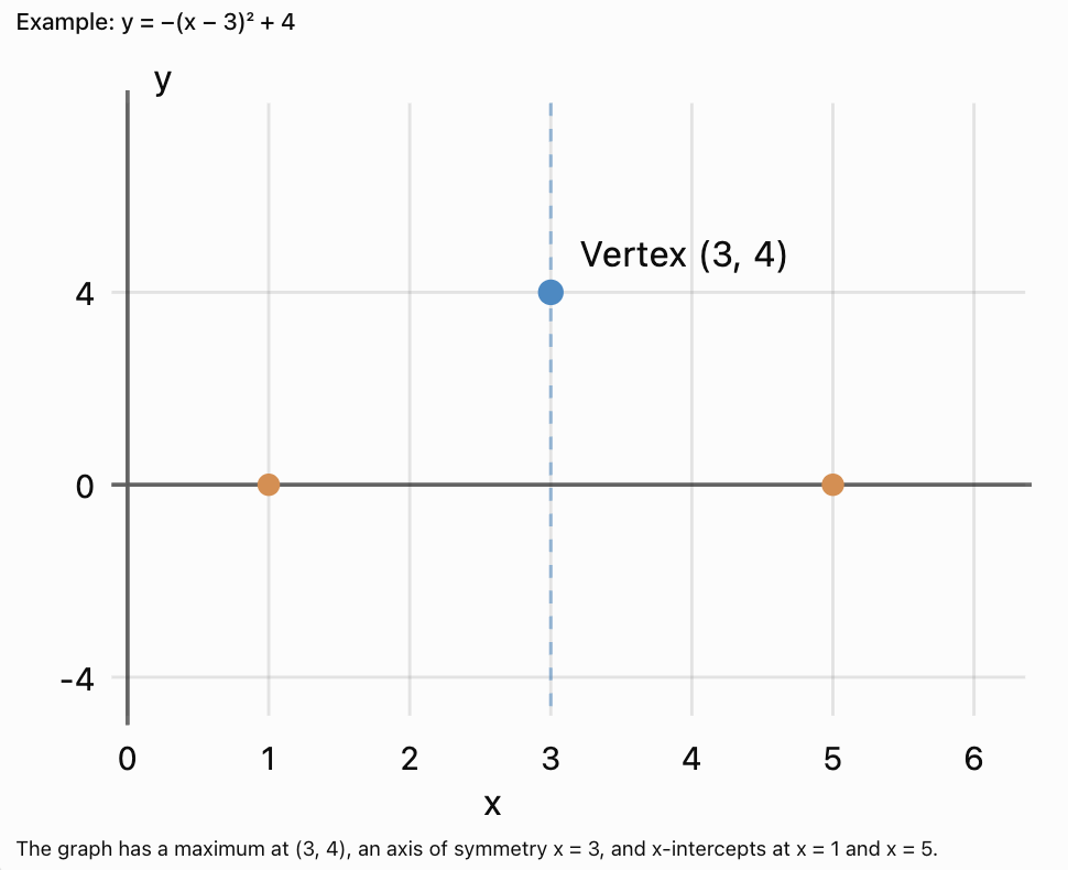
Multi-Step Problem: Rectangular Garden
A gardener has 48 metres of fencing and wants to create a rectangular garden.
Find the dimensions that produce the maximum area.

Step 1: Define Variables
Let:
w = width in metres
l = length in metres
A = area in square metres
Step 2: Write the Perimeter Equation
2w + 2l = 48
Divide by 2:
w + l = 24
Rearrange:
l = 24 − w
Step 3: Create the Area Function
A = lw
A = w(24 − w)
A(w) = −w² + 24w
Step 4: Find the Vertex
w = −24/[2(−1)]
w = 12 m
Step 5: Find the Length
l = 24 − 12
l = 12 m
Step 6: Calculate the Area
A = 12 × 12
A = 144 m²
Step 7: Interpret
The maximum garden area is 144 m², achieved with a square measuring 12 m by 12 m.
Step 8: Evaluate Reasonableness
Check the perimeter:
2(12) + 2(12) = 48 m
The dimensions satisfy the fencing restriction.
The answer is reasonable.
Multi-Step Problem: Projectile Motion
A ball is launched upward from a platform 5 metres high.
Its height is modelled by:
h(t) = −5t² + 25t + 5
where t is time in seconds and h is height in metres.
Find the maximum height and the time when the ball reaches the ground.

Finding Maximum Height
The vertex occurs at:
t = −b/(2a)
t = −25/[2(−5)]
t = 2.5 seconds
Substitute:
h(2.5) = −5(2.5)² + 25(2.5) + 5
h(2.5) = −31.25 + 62.5 + 5
Maximum height = 36.25 m
Finding Landing Time
Set height equal to zero:
0 = −5t² + 25t + 5
Divide by −5:
t² − 5t − 1 = 0
Use the quadratic formula:
t = [5 ± √(25 + 4)]/2
t = [5 ± √29]/2
The two solutions are approximately:
t ≈ 5.19
t ≈ −0.19
Reject the negative time because it occurs before launch.
Final Answer
The ball reaches a maximum height of 36.25 metres after 2.5 seconds.
It reaches the ground approximately 5.19 seconds after launch.
Evaluating Reasonableness
The ball begins 5 metres above ground level.
It rises to a maximum and then falls.
The landing time is greater than the time to maximum height, which is consistent with the situation.
Multi-Step Problem: Business Profit
A business models its profit using:
P(x) = −2x² + 40x − 100
where x is the number of products sold and P is profit in dollars.
Find the number of products that maximises profit and determine the maximum profit.
Step 1: Identify the Goal
We need to find the maximum profit.
Since a = −2, the parabola opens downward.
Step 2: Find the Vertex
x = −40/[2(−2)]
x = 10
Step 3: Calculate Profit
P(10) = −2(10)² + 40(10) − 100
P(10) = −200 + 400 − 100
P(10) = $100
Interpretation
The model predicts a maximum profit of $100 when 10 products are sold.
Reasonableness Check
The optimal quantity is a whole number.
It is also positive.
The answer is reasonable under the assumptions of the model.
Multi-Step Problem: Constructing a Quadratic Equation
A parabola has vertex (2, −3) and passes through (4, 5).
Find its equation.
Step 1: Choose Vertex Form
y = a(x − h)² + k
Since the vertex is (2, −3):
y = a(x − 2)² − 3
Step 2: Substitute the Known Point
Use (4, 5):
5 = a(4 − 2)² − 3
5 = 4a − 3
8 = 4a
a = 2
Step 3: Write the Equation
y = 2(x − 2)² − 3
Step 4: Check
Substitute x = 4:
y = 2(4 − 2)² − 3
y = 2(4) − 3
y = 5
The equation passes through the required point.
Multi-Step Problem: Solving a Quadratic Inequality
Solve:
x² − 5x + 6 < 0
Step 1: Factor
(x − 2)(x − 3) < 0
Step 2: Find the Roots
x = 2
x = 3
Step 3: Analyse the Graph
The parabola opens upward.
It is below the x-axis between its two roots.
Final Answer
2 < x < 3
Important Observation
Quadratic inequalities describe intervals where a function is positive, negative, or equal to zero.
Multi-Step Problem: Comparing Two Functions
Consider:
f(x) = x² − 4x + 3
g(x) = −x² + 6x − 5
Compare their vertices, directions of opening, and x-intercepts.
Function f(x)
Vertex:
x = −(−4)/[2(1)] = 2
f(2) = 4 − 8 + 3 = −1
Vertex:
(2, −1)
Factor:
f(x) = (x − 1)(x − 3)
Roots:
x = 1 and x = 3
Opens upward.
Function g(x)
Vertex:
x = −6/[2(−1)] = 3
g(3) = −9 + 18 − 5 = 4
Vertex:
(3, 4)
Factor:
g(x) = −(x − 1)(x − 5)
Roots:
x = 1 and x = 5
Opens downward.
Comparison
|
Property |
f(x) |
g(x) |
|---|---|---|
|
Vertex |
(2, −1) |
(3, 4) |
|
Opening |
Upward |
Downward |
|
Extremum |
Minimum −1 |
Maximum 4 |
|
x-intercepts |
1 and 3 |
1 and 5 |
|
Axis of symmetry |
x = 2 |
x = 3 |
Communicating Mathematical Reasoning Clearly
A correct answer should be supported by a logical explanation.
A Strong Mathematical Solution Includes
-
A clear statement of what is being found.
-
Appropriate variable definitions.
-
The relevant equation or formula.
-
Correct substitution and calculations.
-
Logical steps.
-
A final answer with units when needed.
-
An explanation of what the answer means.
-
A reasonableness check.
Example
Problem: Find the maximum value of y = −x² + 8x − 5.
A weak answer:
"11"
A stronger answer:
"The coefficient of x² is negative, so the parabola opens downward and has a maximum at its vertex. Using x = −b/(2a), the vertex occurs at x = 4. Substituting gives y = −16 + 32 − 5 = 11. Therefore, the maximum value is 11 when x = 4."
Important Observation
Clear reasoning demonstrates understanding and allows another person to follow and verify the solution.
Evaluating the Reasonableness of Answers
A mathematically correct calculation may still produce an unrealistic result.
Check the Sign
Can the quantity be negative?
For example, a negative garden width is impossible.
Check the Units
Does the answer have appropriate units?
Area should be measured in square units.
Check the Domain
Does the solution lie within the permitted range?
Check the Context
Does the answer make practical sense?
A business cannot normally sell 12.5 individual products.
Check by Substitution
Does the calculated value satisfy the original equation?
Check with a Graph
Does the solution agree with the graph's shape, intercepts, and vertex?
Check by Estimation
Is the answer close to what we would expect?
Important Observation
Reasonableness checks are an essential part of mathematical problem solving, not an optional final step.
A General Strategy for Multi-Step Problems
-
Understand: Identify what is given and what must be found.
-
Represent: Define variables and construct equations, tables, or diagrams.
-
Choose: Select an appropriate mathematical method.
-
Solve: Carry out calculations logically and accurately.
-
Interpret: Explain what the solutions mean in context.
-
Verify: Check calculations, constraints, units, and reasonableness.
-
Communicate: Present a clear final answer supported by reasoning.
Common Mistakes
-
Using the wrong method: Choose factoring, vertex calculations, square roots, or the quadratic formula based on the problem.
-
Forgetting to set the equation equal to zero: This is necessary when solving for roots.
-
Ignoring the negative square root: Square-root equations may have two solutions.
-
Making sign errors: Pay attention to negative coefficients.
-
Confusing the vertex coordinates: The x-coordinate gives the input; the y-coordinate gives the extremum.
-
Ignoring constraints: Not all mathematical solutions are physically possible.
-
Forgetting units: Always include units in contextual answers.
-
Failing to check solutions: Substitute answers back into the original equation.
-
Rounding too early: Keep exact values during calculations when practical.
-
Providing an answer without reasoning: Show enough steps to justify the result.
Key Terms
-
Quadratic Function: Function whose highest variable power is two.
-
Parabola: Graph of a quadratic function.
-
Standard Form: y = ax² + bx + c.
-
Vertex Form: y = a(x − h)² + k.
-
Factored Form: y = a(x − r₁)(x − r₂).
-
Vertex: Maximum or minimum point of a parabola.
-
Axis of Symmetry: Vertical line through the vertex.
-
Root: Value of x that makes a quadratic expression equal to zero.
-
x-Intercept: Point where a graph crosses or touches the x-axis.
-
Discriminant: Expression b² − 4ac.
-
Quadratic Formula: Formula used to solve quadratic equations.
-
Factoring: Rewriting an expression as a product.
-
Completing the Square: Method for rewriting a quadratic expression in vertex form.
-
Optimisation: Finding the best possible value under given conditions.
-
Maximum Value: Greatest output of a function.
-
Minimum Value: Smallest output of a function.
-
Constraint: Restriction on permitted values.
-
Domain: Set of permitted input values.
-
Range: Set of possible output values.
-
Mathematical Model: Mathematical representation of a real-world relationship.
-
Reasonableness Check: Evaluation of whether an answer is mathematically and contextually sensible.
-
Substitution: Replacing a variable with a value or expression.
-
Mathematical Reasoning: Logical explanation supporting a mathematical conclusion.
Key Takeaways
-
Quadratic functions can be written in standard, vertex, or factored form.
-
Different forms are useful for different problems.
-
Factoring is useful when the quadratic expression factors easily.
-
The quadratic formula works for any quadratic equation.
-
The discriminant identifies the number of distinct real roots.
-
The vertex provides the maximum or minimum of an unrestricted quadratic function.
-
Vertex form reveals transformations and the vertex.
-
Quadratic functions can model practical situations such as area, profit, and projectile motion.
-
Multi-step problems require logical organisation and appropriate method selection.
-
Solutions must be interpreted using the problem's context.
-
Constraints may eliminate some mathematical solutions.
-
Units should be included in practical answers.
-
Substitution and estimation help verify results.
-
Clear mathematical communication is an important problem-solving skill.
Check Your Understanding
Choosing Methods
-
Which method is often most efficient for solving x² − 9 = 0?
-
Which form is most useful for identifying the vertex directly?
-
Which method can solve a quadratic equation that does not factor easily?
-
What does the discriminant tell us?
-
Why is choosing an appropriate method important?
Solving Quadratic Equations
-
Solve x² − 5x + 6 = 0.
-
Solve x² − 16 = 0.
-
Solve 2x² − 8x = 0.
-
Find the discriminant of x² + 4x + 4 = 0.
-
Determine the number of distinct real solutions of x² + 2x + 5 = 0.
Vertex and Graphs
-
Find the vertex of y = x² − 6x + 8.
-
Find the maximum value of y = −x² + 8x − 3.
-
Determine the axis of symmetry of y = 2(x − 4)² + 1.
-
Describe the transformations in y = −3(x + 2)² + 5.
-
Find the x-intercepts of y = x² − 7x + 12.
Practical Problems
-
A rectangular garden has perimeter 32 m. What dimensions maximise its area?
-
Find the maximum area in Question 16.
-
A projectile follows h(t) = −5t² + 20t. Find its maximum height.
-
Explain why negative time solutions may be rejected in projectile problems.
-
Give two ways to check whether a quadratic solution is reasonable.
Answer Key
|
Question |
Answer |
|---|---|
|
1 |
Square roots or difference-of-squares factoring |
|
2 |
Vertex form |
|
3 |
Quadratic formula |
|
4 |
Number of distinct real roots |
|
5 |
It makes solving more efficient and reduces errors |
|
6 |
x = 2 or 3 |
|
7 |
x = −4 or 4 |
|
8 |
x = 0 or 4 |
|
9 |
0 |
|
10 |
No real solutions |
|
11 |
(3, −1) |
|
12 |
13 |
|
13 |
x = 4 |
|
14 |
Left 2, reflect, stretch by 3, up 5 |
|
15 |
x = 3 and x = 4 |
|
16 |
8 m by 8 m |
|
17 |
64 m² |
|
18 |
20 m |
|
19 |
They may represent times before launch |
|
20 |
Substitution, graphing, estimation, checking units or constraints |
Extended Challenge
-
Solve 3x² − 11x + 6 = 0.
-
Solve x² + 6x + 13 = 0 over the real numbers.
-
Find the vertex of y = −2x² + 12x − 7.
-
Rewrite y = x² − 10x + 21 in vertex form.
-
Determine the x-intercepts of y = 2x² − 8x + 6.
-
Solve the inequality x² − 4x − 5 ≤ 0.
-
A rectangle has perimeter 60 m. Find its maximum area.
-
A business has profit P(x) = −4x² + 80x − 200. Find the maximum profit.
-
A projectile follows h(t) = −5t² + 30t + 10. Find the maximum height and the time it occurs.
-
A parabola has vertex (−2, 5) and passes through (0, −3). Find its equation.
Final Investigation: Quadratic Problem-Solving Challenge
Complete the following investigation using a variety of mathematical methods.
Part A: Algebraic Skills
-
Solve x² − 9x + 20 = 0 by factoring.
-
Solve 2x² + 5x − 3 = 0 using the quadratic formula.
-
Find the discriminant of 3x² − 6x + 3 = 0.
-
Determine the vertex of y = x² − 8x + 10.
-
Rewrite y = x² + 4x − 5 in vertex form.
Part B: Graph Analysis
Consider:
f(x) = −2(x − 3)² + 8
-
Identify the vertex.
-
Determine the axis of symmetry.
-
Describe all transformations from y = x².
-
Determine the maximum value.
-
Find the x-intercepts.
Part C: Real-World Modelling
A rectangular garden has 40 metres of fencing.
-
Define suitable variables.
-
Write the perimeter equation.
-
Construct a quadratic area function.
-
Determine the dimensions that maximise area.
-
Calculate the maximum area.
Part D: Projectile Motion
A ball is launched from a height of 3 metres.
Its height is:
h(t) = −5t² + 20t + 3
-
Determine the initial height.
-
Find the time at maximum height.
-
Calculate the maximum height.
-
Determine when the ball reaches the ground, to two decimal places.
-
Evaluate whether the calculated answers are reasonable.
Selected Investigation Answers
Part A
-
x = 4 or 5
-
x = 0.5 or −3
-
D = 0
-
Vertex (4, −6)
-
y = (x + 2)² − 9
Part B
-
Vertex (3, 8)
-
x = 3
-
Right 3, vertical stretch 2, reflect across the x-axis, up 8
-
Maximum value = 8
-
x = 1 or 5
Part C
-
A(w) = −w² + 20w
-
10 m by 10 m
-
100 m²
Part D
-
3 m
-
2 s
-
23 m
-
Approximately 4.14 s
-
The ball begins 3 m above ground, rises to a maximum, and then reaches the ground after a positive amount of time. These results are consistent with the model.