Advanced Exponential and Logarithmic Models
3. Continuous Growth and Decay
Learning outcomes
- I can model continuously compounded growth.
- I can model continuous decay.
- I can compare discrete and continuous models.
- I can interpret continuous growth models.
- I can solve authentic applications.
Introduction
Imagine investing money in a savings account that earns interest continuously. As the account balance grows, the amount of interest earned also increases because interest is calculated on an increasingly large balance.
Now imagine a radioactive substance gradually losing mass as its unstable nuclei decay. The amount that decays during a particular interval depends on how much radioactive material remains.
Although these situations appear different, they can be described using the same mathematical principle: the rate of change of a quantity is proportional to the quantity currently present.
This principle leads to continuous exponential growth and decay models.
These models are used in finance, population biology, medicine, chemistry, physics, and environmental science. They allow us to predict future quantities, calculate doubling times and half-lives, compare different growth processes, and solve practical problems involving time and rates of change.
Understanding Continuous Growth and Decay
A quantity experiences continuous exponential growth when its instantaneous rate of increase is proportional to its current value.
A quantity experiences continuous exponential decay when its instantaneous rate of decrease is proportional to its current value.
Both processes can be represented by:
Where:
-
Q(t) = quantity at time t
-
Q₀ = initial quantity
-
e = Euler's number, approximately 2.71828
-
k = continuous growth or decay constant
-
t = elapsed time
The sign of k determines the behaviour.
|
Value of k |
Behaviour |
|---|---|
|
k > 0 |
Exponential growth |
|
k = 0 |
Constant quantity |
|
k < 0 |
Exponential decay |
The units of k are the reciprocal of the time unit. For example, if t is measured in years, k is measured per year.
Why is the model called continuous?
In a continuous model, the quantity changes throughout time rather than only at separate intervals.
The underlying mathematical relationship is:
This means that the instantaneous rate of change is proportional to the current quantity.
For example, if a population contains twice as many organisms, its instantaneous growth rate is twice as large, provided k remains constant.
Visualising Continuous Growth and Decay
Consider two quantities, both initially equal to 100.
One grows with k = 0.25, while the other decays with k = −0.25.
Their models are:
Growth: Q(t) = 100e^(0.25t)
Decay: Q(t) = 100e^(−0.25t)
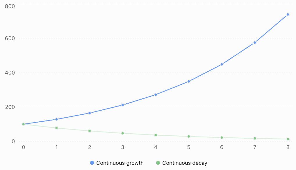
Notice that:
-
Both quantities begin at 100.
-
The growing quantity increases by larger absolute amounts over successive equal time intervals.
-
The decaying quantity decreases, but its absolute losses become smaller.
-
The decay model approaches zero without reaching it in finite time.
-
Both processes have a constant proportional rate of change, even though their absolute rates change.
The constant proportional rate is the defining feature of exponential growth and decay.
Developing Continuous Growth Models
Suppose a population initially contains 500 organisms and grows continuously at a rate of 8% per year.
The initial quantity is:
Q₀ = 500
The continuous growth constant is:
k = 0.08 per year
Therefore:
Worked Example 1: Predicting Population Growth
Estimate the population after 6 years.
Step 1: Write the model.
Step 2: Substitute t = 6.
Step 3: Evaluate.
The predicted population after six years is approximately 808 organisms.
Interpreting the result
The population has increased from 500 to approximately 808.
The absolute increase is:
808 − 500 = 308 organisms.
The continuous growth constant remains 0.08 per year, but the population's instantaneous absolute growth rate increases as the population becomes larger.
This distinction between proportional growth and absolute growth is important.
Continuously Compounded Interest
One of the best-known applications of continuous exponential growth is compound interest.
With ordinary compound interest, interest is added at specified intervals, such as annually, monthly, or daily.
With continuous compounding, we consider the limiting situation as the compounding frequency increases without bound.
The continuously compounded interest formula is:
Where:
-
A = final account balance
-
P = principal, or initial investment
-
r = nominal annual interest rate expressed as a decimal
-
t = time in years
Explore continuous compound interest
Change the initial investment, annual interest rate, or investment period to explore how continuous compounding affects the final balance.Worked Example 2: Continuous Compound Interest
An investment of $6,000 earns interest at a nominal annual rate of 4.5%, compounded continuously.
Calculate the value after 8 years.
Step 1: Identify the values.
P = 6000
r = 0.045
t = 8
Step 2: Substitute.
Step 3: Evaluate.
Step 4: Calculate the interest earned.
The investment earns approximately $2,599.98 in interest over eight years, assuming the rate remains constant and there are no deposits, withdrawals, taxes, or fees.
Continuous Exponential Decay
Exponential decay occurs when a quantity decreases at a rate proportional to the amount remaining.
A convenient decay model is:
Where λ is a positive decay constant.
This is equivalent to the general model Q(t) = Q₀eᵏᵗ with k = −λ.
Examples include:
-
Radioactive decay.
-
Certain chemical reactions.
-
Drug elimination under first-order conditions.
-
Capacitor discharge.
-
Temperature differences during Newtonian cooling.
Worked Example 3: Decaying Substance
A substance initially has a mass of 400 g and decays continuously at a rate of 12% per hour.
Calculate its remaining mass after 5 hours.
Step 1: Write the model.
Step 2: Substitute t = 5.
Step 3: Evaluate.
Step 4: Calculate the mass lost.
Approximately 180.48 g has been lost.
The mass remaining is always positive in this idealised model.
Comparing Discrete and Continuous Growth
Exponential growth can be modelled using discrete or continuous approaches.
Discrete growth
Discrete growth uses a constant multiplier over each complete time period.
The model is:
Where:
-
Q₀ = initial quantity
-
r = effective growth rate per period
-
n = number of periods
For example, if a population grows by exactly 5% each year:
Continuous growth
Continuous growth uses the natural exponential function:
Here, k is the continuous relative growth rate.
Although these models look different, they can describe the same values at whole-number times.
Converting between growth rates
The relationship is:
Therefore:
and:
These formulas are essential for comparing discrete and continuous growth rates.
Worked Example 4: Converting a Discrete Rate to a Continuous Rate
A population increases by exactly 6% each year.
Find the equivalent continuous growth rate.
The annual growth multiplier is:
Therefore:
The equivalent continuous growth rate is approximately 5.827% per year.
The models:
Q = Q₀(1.06)ⁿ
and
Q(t) = Q₀e^(0.05827t)
produce the same quantities at integer-year times, apart from rounding.
Worked Example 5: Converting a Continuous Rate to an Effective Annual Rate
An investment grows continuously at 8% per year.
Find its effective annual growth rate.
A continuous rate of 8% per year corresponds to an effective annual increase of approximately 8.329%.
It is not exactly an 8% annual increase.
Comparing Compounding Frequencies
For a nominal annual interest rate r compounded m times per year:
As m becomes increasingly large, the expression approaches continuous compounding.
Consider $1,000 invested at a nominal annual interest rate of 10% for one year.
|
Compounding frequency |
Final amount |
|---|---|
|
Annually |
$1,100.00 |
|
Semiannually |
$1,102.50 |
|
Quarterly |
$1,103.81 |
|
Monthly |
$1,104.71 |
|
Daily (365 times) |
$1,105.16 |
|
Continuously |
$1,105.17 |
More frequent compounding produces a larger balance when the nominal rate is positive.
However, the additional benefit becomes smaller as the frequency increases.
The chart compares interest earned rather than total balances, making the relatively small differences easier to see.
Comparing Discrete and Continuous Decay
Discrete decay uses a constant percentage reduction during each time period.
For a fractional decay rate d per period:
where 0 < d < 1.
Continuous decay uses:
The equivalent rates satisfy:
Therefore:
Worked Example 6: Converting a Decay Rate
A substance loses exactly 15% of its mass each day.
Find the equivalent continuous decay constant.
The daily remaining fraction is:
Therefore:
The corresponding continuous decay model is:
This model matches the discrete model at whole-day times, subject to rounding.
The continuous decay constant is approximately 0.16252 per day, not 0.15 per day.
Interpreting Continuous Growth Models
A continuous exponential model provides more information than simply the predicted quantity.
Consider:
where t is measured in years.
We can interpret its components.
Initial quantity
At t = 0:
The initial population is 2,500.
Continuous growth rate
The constant k = 0.035 indicates a continuous relative growth rate of 3.5% per year.
Instantaneous rate of change
Differentiate the model:
Therefore:
At t = 0:
The population is initially increasing at an instantaneous rate of 87.5 organisms per year.
When the population reaches 4,000:
Its instantaneous growth rate becomes 140 organisms per year.
The relative growth rate remains constant, but the absolute growth rate increases.
Instantaneous rate versus average rate
The instantaneous rate describes how quickly the quantity is changing at a particular moment.
The average rate of change over an interval is:
These are generally different for exponential functions.
This distinction is especially important in calculus and mathematical modelling.
Doubling Time
The doubling time is the time required for a continuously growing quantity to become twice its initial value.
Starting with:
At doubling:
Divide by Q₀:
Take natural logarithms:
Therefore:
where k > 0.
Worked Example 7: Calculating Doubling Time
A population grows continuously at 4.5% per year.
Calculate its doubling time.
The population doubles approximately every 15.4 years if the growth constant remains unchanged.
Notice that doubling time does not depend on the initial population.
A population of 500 and a population of 50,000 have the same doubling time when they share the same constant k.
Half-Life
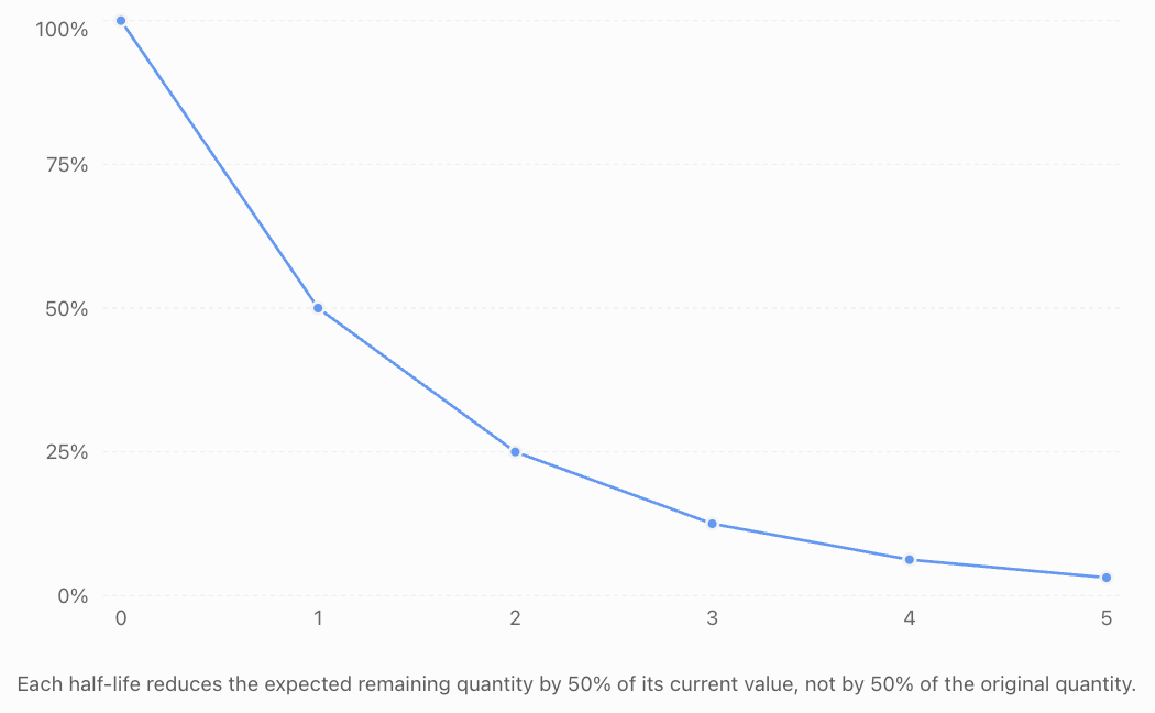
The half-life is the time required for an exponentially decaying quantity to decrease to half its initial value.
For:
the half-life is:
where λ > 0.
Worked Example 8: Radioactive Half-Life
A radioactive substance has a decay constant of 0.075 per year.
Calculate its half-life.
After approximately 9.24 years, half the original radioactive nuclei are expected to remain.
After two half-lives, one-quarter remain.
After three half-lives, one-eighth remain.
Exponential decay over successive half-lives
Finding the Growth or Decay Constant from Data
Sometimes the initial and final quantities are known, but the growth or decay constant is unknown.
Start with:
Divide by Q₀:
Take natural logarithms:
Rearrange:
This formula allows us to determine the continuous rate from observations.
Worked Example 9: Finding a Growth Constant
A population increases from 800 to 1,200 over five years.
Assuming continuous exponential growth, calculate k.
The continuous growth rate is approximately 8.109% per year.
The model becomes:
Worked Example 10: Finding a Decay Constant
A substance decreases from 300 g to 180 g over four hours.
Find its continuous decay constant.
The signed growth constant is −0.12771 per hour.
Equivalently, the positive decay constant is:
The model is:
Solving Authentic Applications
Continuous exponential models become particularly useful when the unknown is time, a growth rate, or an initial quantity.
Application 1: Medicine — Drug Elimination
A medication has an initial amount of 200 mg in the body.
Under an idealised first-order elimination model, the amount remaining is:
where t is measured in hours.
How long will it take for the amount to decrease to 50 mg?
Step 1: Substitute the target amount.
Step 2: Divide by 200.
Step 3: Take natural logarithms.
Step 4: Solve.
The model predicts that the amount decreases to 50 mg after approximately 7.70 hours.
Actual drug elimination depends on the medication, individual physiology, and whether first-order kinetics apply. This calculation is a mathematical illustration, not a dosing recommendation.
Application 2: Finance — Reaching a Savings Goal
An investor deposits $10,000 into an account earning 5% nominal annual interest compounded continuously.
How long will it take for the account to reach $15,000?
Divide by 10,000:
Take natural logarithms:
The investment reaches $15,000 after approximately 8.11 years under the assumed constant rate.
Application 3: Environmental Science — Pollutant Removal
A pollutant has an initial concentration of 80 mg/L.
Its concentration decreases continuously according to:
where t is measured in days.
Determine when the concentration falls to 10 mg/L.
The model predicts that the concentration reaches 10 mg/L after approximately 6.93 days.
This assumes a constant proportional removal rate, with no additional pollutant entering the system.
Application 4: Physics — Newton's Law of Cooling
A hot object cools in a room maintained at a constant temperature.
Under suitable conditions, Newton's law of cooling gives:
Where:
-
T(t) = temperature at time t
-
Tₐ = ambient temperature
-
T₀ = initial object temperature
-
k = positive cooling constant
Suppose a cup of coffee begins at 90°C in a room at 22°C, with k = 0.12 per minute.
Find its temperature after 10 minutes.
The coffee is predicted to cool to approximately 42.5°C.
Notice that the temperature difference from the surroundings, rather than the absolute temperature, follows an exponential decay model.
Evaluating Model Assumptions and Limitations
Continuous exponential models are useful, but they depend on important assumptions.
Constant proportional rate
The model assumes that k remains constant.
Real population growth may slow because of limited resources.
Investment rates may change over time.
Drug elimination may not always follow first-order kinetics.
Appropriate time interval
An exponential model may work well over a short period but become unrealistic over a much longer period.
For example, a bacterial population cannot grow exponentially forever in a closed container.
No unmodelled additions or removals
A simple decay model assumes the quantity is not replenished.
If additional pollutants enter a river, a basic exponential decay model may no longer describe the situation adequately.
Reliable measurements
Estimated growth and decay constants depend on the quality of the data.
Measurement error, missing observations, and inappropriate assumptions can produce misleading predictions.
Discrete versus continuous reality
Some processes occur through individual events but can still be modelled using continuous equations.
For example, radioactive nuclei decay individually, but the expected number remaining in a large sample follows an exponential law.
A continuous model is a mathematical description of the overall behaviour, not necessarily a claim that every underlying event occurs continuously.
Common Mistakes
Mistake 1: Confusing continuous and effective growth rates
A continuous growth rate of 5% does not mean exactly 5% growth over one year.
Correction: Use r = eᵏ − 1 to calculate the effective growth rate over one time unit.
Mistake 2: Using the wrong sign for decay
The expression Q = Q₀e⁰·¹ᵗ represents growth, not decay.
Correction: Use a negative exponent coefficient for decay.
Mistake 3: Mixing time units
A decay constant measured per hour cannot be used directly with time measured in days.
Correction: Convert time units before substituting.
Mistake 4: Treating half-life as a constant absolute decrease
After each half-life, half the current amount remains.
Correction: Apply a multiplicative factor of 0.5, not a fixed subtraction.
Mistake 5: Confusing continuous compounding with monthly compounding
These are different models.
Correction: Use A = Peʳᵗ for continuous compounding and A = P(1 + r/m)ᵐᵗ for m compounding periods per year.
Mistake 6: Forgetting logarithms when solving for time
When the unknown appears in the exponent, ordinary linear rearrangement is insufficient.
Correction: Isolate the exponential expression and take natural logarithms.
Mistake 7: Applying exponential models indefinitely
Many real processes change behaviour as conditions change.
Correction: Consider whether the model's assumptions remain valid over the prediction period.
Key Terms
-
Continuous Growth: Growth in which the instantaneous rate of increase is proportional to the current quantity.
-
Continuous Decay: Decrease in which the instantaneous rate of decrease is proportional to the current quantity.
-
Euler's Number (e): An irrational constant approximately equal to 2.71828.
-
Initial Quantity: The amount present at time zero.
-
Growth Constant: The positive parameter k in an exponential growth model.
-
Decay Constant: The positive parameter λ in an exponential decay model.
-
Continuous Compounding: The limiting form of compound interest as compounding frequency increases without bound.
-
Discrete Growth: Growth represented using fixed percentage changes over separate time periods.
-
Effective Growth Rate: The actual proportional increase over a specified time interval.
-
Instantaneous Rate of Change: The rate at which a quantity changes at a particular moment.
-
Relative Growth Rate: The instantaneous rate of change divided by the current quantity.
-
Doubling Time: The time required for an exponentially growing quantity to double.
-
Half-Life: The time required for an exponentially decaying quantity to halve.
-
Natural Logarithm: A logarithm with base e, written ln(x).
-
Exponential Model: A mathematical relationship in which a variable appears in an exponent.
-
First-Order Decay: A process in which the rate of decrease is proportional to the amount remaining.
-
Mathematical Assumption: A condition required for a model or method to be appropriate.
-
Extrapolation: Using a model to predict beyond the range of observed data.
Key Takeaways
-
Continuous growth and decay are modelled using Q(t) = Q₀eᵏᵗ.
-
Positive k represents growth; negative k represents decay.
-
Continuous compounding is modelled by A = Peʳᵗ.
-
Discrete growth uses Qₙ = Q₀(1 + r)ⁿ.
-
The equivalent discrete and continuous rates satisfy k = ln(1 + r).
-
Continuous decay can be written as Q(t) = Q₀e⁻λᵗ.
-
The equivalent discrete decay fraction satisfies λ = −ln(1 − d).
-
The instantaneous rate of change is proportional to the current quantity.
-
Doubling time is ln(2)/k for positive k.
-
Half-life is ln(2)/λ for positive λ.
-
Natural logarithms allow us to solve for time and growth constants.
-
Continuous exponential models are useful in finance, biology, medicine, chemistry, physics, and environmental science.
-
All predictions should be interpreted in the context of the model's assumptions and limitations.
Check Your Understanding
Questions
Question 1: Identifying Growth and Decay
Determine whether each model represents growth or decay.
a) Q(t) = 500e^(0.06t)
b) Q(t) = 800e^(−0.09t)
c) Q(t) = 200e^(0t)
Question 2: Continuous Population Growth
A population initially contains 1,500 organisms and grows continuously at 4% per year.
Write a model and calculate the population after 8 years.
Question 3: Continuous Compound Interest
An investment of $7,500 earns 5% annual interest compounded continuously.
Calculate its value after 12 years.
Question 4: Continuous Decay
A substance initially has a mass of 600 g and decays continuously at a rate of 8% per hour.
Calculate the remaining mass after 7 hours.
Question 5: Discrete to Continuous Growth
A population increases by exactly 7% annually.
Find the equivalent continuous growth constant.
Question 6: Continuous to Discrete Growth
An investment grows continuously at 6% per year.
Calculate its effective annual growth rate.
Question 7: Doubling Time
A population grows continuously at 3% per year.
Calculate its doubling time.
Question 8: Half-Life
A substance has a decay constant of 0.11 per day.
Calculate its half-life.
Question 9: Finding a Growth Constant
A population increases from 2,000 to 3,000 over 6 years.
Assuming continuous exponential growth, calculate the growth constant.
Question 10: Finding Time
A substance decays according to:
How long will it take for the mass to decrease to 125 g?
Question 11: Comparing Models
Explain the difference between:
Q(t) = 1000(1.05)ᵗ
and
Q(t) = 1000e^(0.05t).
Do they represent the same growth rate?
Question 12: Authentic Application
A lake contains a pollutant at a concentration of 120 mg/L. Its concentration decreases continuously at 18% per day.
Write a model and calculate when the concentration reaches 30 mg/L.
Question 13: Interpreting a Model
Consider:
Explain the meaning of 4000 and 0.025. Calculate the instantaneous growth rate when the population is 6,000.
Question 14: Evaluating Model Limitations
A scientist models a bacterial population using exponential growth and predicts that it will increase indefinitely.
Explain two reasons why this prediction may eventually become unrealistic.
Fully Worked Answers
Answer 1: Identifying Growth and Decay
a) k = 0.06, which is positive.
Exponential growth.
b) k = −0.09, which is negative.
Exponential decay.
c) k = 0.
The quantity remains constant at 200.
Answer 2: Continuous Population Growth
The model is:
After 8 years:
The predicted population is approximately 2,066 organisms.
Answer 3: Continuous Compound Interest
Use:
Substitute:
Answer 4: Continuous Decay
After 7 hours:
Answer 5: Discrete to Continuous Growth
The annual growth rate is r = 0.07.
The equivalent continuous growth rate is approximately 6.766% per year.
Answer 6: Continuous to Discrete Growth
Given k = 0.06:
The effective annual growth rate is approximately 6.184%.
Answer 7: Doubling Time
Answer 8: Half-Life
Answer 9: Finding a Growth Constant
Substitute:
The continuous growth rate is approximately 6.758% per year.
Answer 10: Finding Time
Divide by 500:
Take natural logarithms:
Rearrange:
The mass decreases to 125 g after approximately 17.33 time units.
Answer 11: Comparing Models
The first model:
represents an effective growth rate of exactly 5% per unit of time.
The second model:
represents a continuous growth rate of 5% per unit of time.
Its effective growth rate over one time unit is:
or approximately 5.127%.
Therefore, the models do not have exactly the same growth rate.
Answer 12: Authentic Application
The initial concentration is 120 mg/L.
The continuous decay constant is 0.18 per day.
The model is:
Set C(t) = 30.
Take natural logarithms:
The concentration reaches 30 mg/L after approximately 7.70 days.
Answer 13: Interpreting a Model
The model is:
The initial population is 4,000.
The continuous growth constant is 0.025, representing a continuous growth rate of 2.5% per time unit.
The instantaneous rate of change is:
When P = 6000:
The population is increasing at an instantaneous rate of 150 organisms per time unit.
Answer 14: Evaluating Model Limitations
Exponential population growth assumes that the relative growth rate remains constant.
This may become unrealistic because:
Limited resources: Nutrients, water, oxygen, or space may become insufficient to support continued growth.
Environmental changes: Waste accumulation, competition, disease, or temperature changes may reduce the growth rate.
A logistic growth model or another model incorporating environmental limits may become more appropriate.
Final Reflection
Continuous growth and decay models provide a powerful connection between exponential functions, natural logarithms, and real-world change.
Their central principle is that the instantaneous rate of change is proportional to the quantity currently present.
This allows us to model investments, populations, radioactive substances, chemical concentrations, and many other processes.
The most important general equation is:
Understanding how to interpret its parameters, compare it with discrete models, and solve for unknown quantities makes continuous exponential modelling a valuable tool across mathematics and science.
A successful mathematical model does more than produce an answer. It provides a meaningful interpretation of a real situation while recognising the assumptions and limitations on which the prediction depends.