Advanced Exponential and Logarithmic Models
| サイト: | Young Education |
| コース: | Exponential and Logarithmic Functions |
| ブック: | Advanced Exponential and Logarithmic Models |
| 印刷者: | Guest user |
| 日付: | 2026年 11月 9日(月曜日) 16:40 |
1. Natural Exponential Functions
Learning outcomes
- I can explain the significance of the number .
- I can evaluate functions involving .
- I can compare natural exponential and other exponential functions.
- I can interpret natural growth models.
- I can apply natural exponential functions to practical situations.
Introduction
Imagine depositing money into a bank account that earns interest continuously. Imagine a population of bacteria growing at a rate proportional to its current size, or a radioactive substance gradually decreasing in mass.
These situations can be modelled using a special mathematical constant called Euler's number, represented by the symbol e.
The number e is one of the most important constants in mathematics. It appears in calculus, finance, biology, chemistry, physics, economics, and statistics.
Its approximate value is:
Like π, the number e is irrational. Its decimal expansion continues forever without repeating.
Exponential functions with base e are called natural exponential functions. They are particularly useful because they describe processes in which the rate of change is proportional to the quantity currently present.
In this lesson, we will investigate the significance of e, evaluate natural exponential functions, compare exponential models, interpret continuous growth and decay, and apply these ideas to practical problems.
Understanding Euler's Number
The constant e arises naturally when investigating continuous growth.
Consider an investment of $1 earning 100% annual interest.
If the interest is added once per year, the balance after one year is:
If interest is compounded twice per year:
If interest is compounded four times per year:
As the number of compounding periods increases, the balance approaches a particular value.
|
Compounding periods per year |
Final balance |
|---|---|
|
1 |
2.000000 |
|
2 |
2.250000 |
|
4 |
2.441406 |
|
12 |
2.613035 |
|
52 |
2.692597 |
|
365 |
2.714567 |
|
10,000 |
2.718146 |
|
Continuous limit |
2.718282 |
The limiting value is e.
Mathematically:
This is one way to define Euler's number.
Approaching Euler's number through compounding
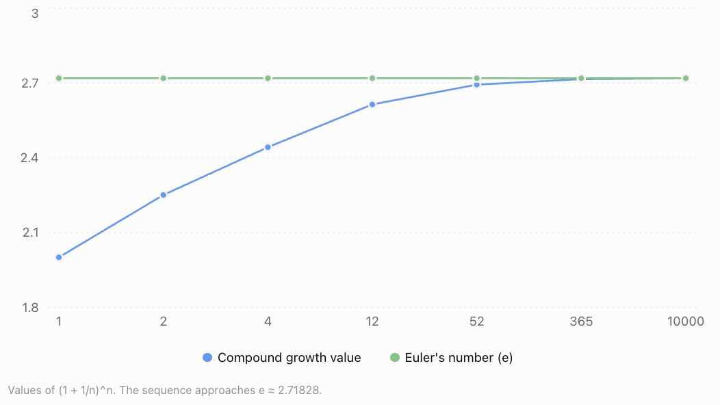
Why is e significant?
The number e has several remarkable properties.
-
It is the natural base for continuous exponential growth and decay.
-
It appears in continuously compounded interest.
-
The function eˣ has a rate of change equal to its own value.
-
Its inverse function is the natural logarithm, ln(x).
-
It appears in probability distributions, differential equations, and many physical models.
The special relationship between eˣ and its rate of change makes natural exponential functions especially important in calculus.
The Natural Exponential Function
The basic natural exponential function is:
Here, e is the constant base and x is the exponent.
The function is defined for every real value of x.
Some useful values are:
|
x |
eˣ (approximately) |
|---|---|
|
−3 |
0.0498 |
|
−2 |
0.1353 |
|
−1 |
0.3679 |
|
0 |
1 |
|
1 |
2.7183 |
|
2 |
7.3891 |
|
3 |
20.0855 |
Properties of y = eˣ
-
Domain: All real numbers.
-
Range: y > 0.
-
y-intercept: (0, 1).
-
Horizontal asymptote: y = 0.
-
The function is continuous and strictly increasing.
-
It has no x-intercepts.
-
As x approaches positive infinity, eˣ increases without bound.
-
As x approaches negative infinity, eˣ approaches zero from above.
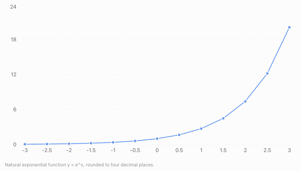
The graph passes through (0, 1) and increases increasingly rapidly as x becomes larger.
Although the curve approaches the x-axis for negative x-values, it never touches or crosses it.
Evaluating Natural Exponential Functions
To evaluate a natural exponential function, substitute the given value into the exponent and calculate.
Most scientific calculators have an eˣ function, often accessed using a secondary function key.
Worked Example 1: Evaluating eˣ
Evaluate:
\[ f(x)=e^{2x} \]when x = 1.5.
Step 1: Substitute the value.
\[ f(1.5)=e^{2(1.5)} \]Step 2: Simplify the exponent.
\[ f(1.5)=e^3 \]Step 3: Evaluate.
\[ \boxed{f(1.5)\approx20.086} \]Worked Example 2: Negative Exponents
Evaluate:
\[ g(x)=5e^{-0.4x} \]when x = 3.
Substitute:
\[ g(3)=5e^{-0.4(3)} \]\[ g(3)=5e^{-1.2} \]Since:
\[ e^{-1.2}\approx0.3010 \]Therefore:
\[ g(3)\approx5(0.3010) \]\[ \boxed{g(3)\approx1.506} \]A negative exponent does not produce a negative exponential value.
Instead:
\[ e^{-x}=\frac1{e^x} \]The result is always positive.
Worked Example 3: Evaluating a Transformed Function
Evaluate:
\[ h(x)=3e^{0.5x}-4 \]when x = 2.
\[ h(2)=3e^{0.5(2)}-4 \]\[ =3e^1-4 \]\[ \approx3(2.71828)-4 \]\[ \boxed{h(2)\approx4.155} \]The subtraction of 4 occurs after evaluating and multiplying the exponential term.
Laws of Exponents
Natural exponential functions follow the same exponent laws as other exponential functions.
For real numbers a and b:
Law
Expression
Product
eᵃ × eᵇ = eᵃ⁺ᵇ
Quotient
eᵃ / eᵇ = eᵃ⁻ᵇ
Power of a power
(eᵃ)ᵇ = eᵃᵇ
Zero exponent
e⁰ = 1
Negative exponent
e⁻ᵃ = 1/eᵃ
Worked Example 4: Simplifying Exponential Expressions
Simplify:
\[ \frac{e^{3x}e^{2x}}{e^x} \]Combine the terms in the numerator.
\[ e^{3x}e^{2x}=e^{5x} \]Now divide.
\[ \frac{e^{5x}}{e^x}=e^{5x-x} \]\[ \boxed{e^{4x}} \]These laws are useful when simplifying exponential models and solving equations.
Comparing Natural Exponential Functions with Other Exponential Functions
A general exponential function has the form:
\[ f(x)=a^x \]where a > 0 and a ≠ 1.
A natural exponential function uses the specific base e:
\[ f(x)=e^x \]Consider three functions:
\[ f(x)=2^x \]\[ g(x)=e^x \]\[ h(x)=3^x \]All three pass through (0, 1), because any positive base raised to the power zero equals 1.
For positive x, larger bases produce larger values.
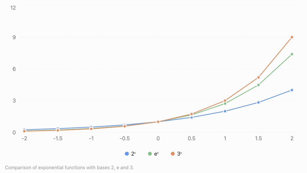
Important comparison
Property
2ˣ
eˣ
3ˣ
Base
2
Approximately 2.718
3
y-intercept
1
1
1
Domain
All real numbers
All real numbers
All real numbers
Range
Positive real numbers
Positive real numbers
Positive real numbers
Behaviour
Growth
Growth
Growth
Derivative
2ˣ ln(2)
eˣ
3ˣ ln(3)
The derivative property is what makes e especially useful.
For any positive base a:
\[ \frac{d}{dx}a^x=a^x\ln(a) \]For a = e:
\[ \ln(e)=1 \]Therefore:
\[ \boxed{\frac{d}{dx}e^x=e^x} \]The function eˣ is its own derivative.
This means its instantaneous rate of change at any point is equal to its value at that point.
Natural Exponential Growth and Decay
Many real-world processes change at a rate proportional to the amount currently present.
These can be modelled by:
\[ \boxed{Q(t)=Q_0e^{kt}} \]Where:
-
Q(t) = quantity at time t
-
Q₀ = initial quantity
-
k = continuous growth or decay rate
-
t = time
Exponential growth
When k > 0:
\[ Q(t)=Q_0e^{kt} \]The quantity increases over time.
Examples include idealised population growth, continuously compounded investments, and early-stage microbial growth under favourable conditions.
Exponential decay
When k < 0:
\[ Q(t)=Q_0e^{kt} \]The quantity decreases over time.
Examples include radioactive decay, drug elimination under certain conditions, and the discharge of a capacitor.
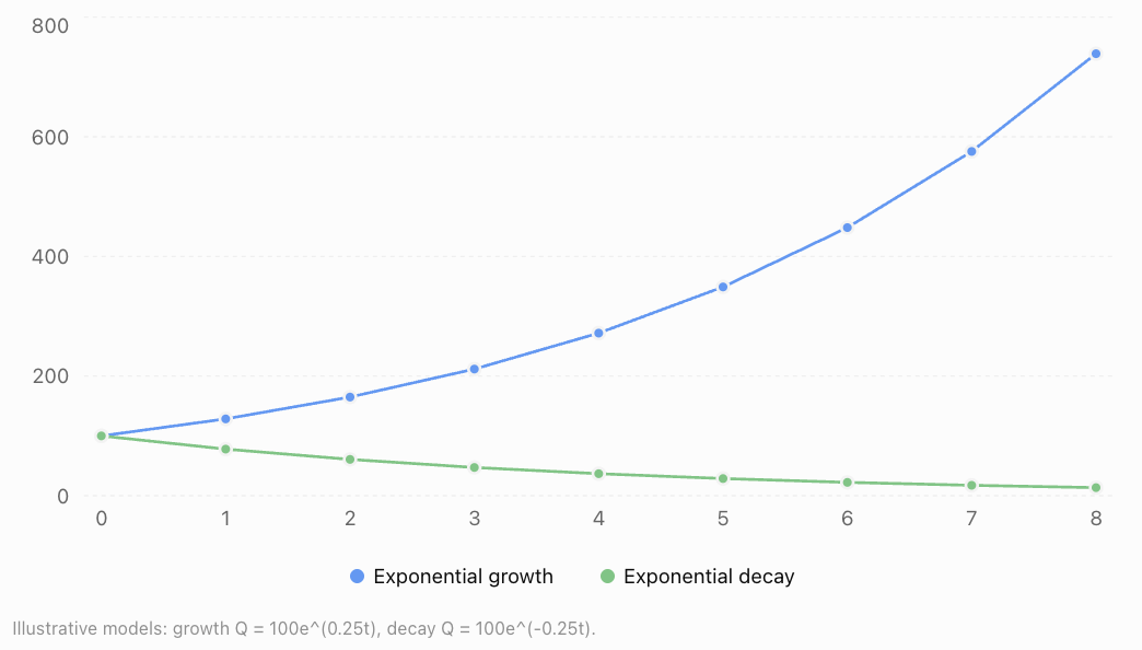
Both models begin at 100, but their values move in opposite directions.
Interpreting the Continuous Growth Rate
The parameter k represents the continuous relative rate of change.
For the model:
\[ Q(t)=Q_0e^{kt} \]the derivative is:
\[ \frac{dQ}{dt}=kQ \]Therefore:
\[ \frac1Q\frac{dQ}{dt}=k \]This shows that the instantaneous rate of change is proportional to the quantity present.
Continuous rate versus percentage growth per period
Suppose:
\[ Q(t)=Q_0e^{0.06t} \]The continuous growth rate is 6% per unit of time.
However, the actual percentage increase over one time unit is:
\[ (e^{0.06}-1)\times100\% \]\[ \approx6.184\% \]Thus, a continuous growth rate of 6% is not exactly the same as a 6% increase per year.
Conversely, if a quantity grows by exactly 6% each year:
\[ Q(t)=Q_0(1.06)^t \]This can be rewritten as:
\[ Q(t)=Q_0e^{t\ln(1.06)} \]The equivalent continuous rate is:
\[ k=\ln(1.06)\approx0.05827 \]or approximately 5.827% per year.
This distinction is important when comparing exponential models.
Converting Between Exponential Forms
Any exponential function with a positive base can be expressed using e.
The key identity is:
\[ \boxed{a^x=e^{x\ln(a)}} \]For example:
\[ 2^x=e^{x\ln2} \]Since ln(2) ≈ 0.6931:
\[ 2^x\approx e^{0.6931x} \]Similarly:
\[ 1.08^t=e^{t\ln(1.08)} \]\[ \approx e^{0.07696t} \]This allows us to compare discrete percentage growth models with continuous exponential growth models.
Continuous Compound Interest
Natural exponential functions are especially useful in financial mathematics.
When interest is compounded continuously:
\[ \boxed{A=Pe^{rt}} \]Where:
-
A = final amount
-
P = principal or initial investment
-
r = annual interest rate as a decimal
-
t = time in years
Worked Example 5: Continuous Interest
An investment of $5,000 earns 4% annual interest, compounded continuously.
Calculate the value after 6 years.
Step 1: Identify the variables.
P = 5000
r = 0.04
t = 6
Step 2: Substitute.
\[ A=5000e^{0.04(6)} \]\[ A=5000e^{0.24} \]Step 3: Evaluate.
\[ A\approx5000(1.271249) \]\[ \boxed{A\approx\$6,356.25} \]The investment grows to approximately $6,356.25.
The interest earned is:
\[ 6356.25-5000=\boxed{\$1,356.25} \]Comparing continuous and annual compounding
With annual compounding:
\[ A=P(1+r)^t \]\[ A=5000(1.04)^6 \]\[ A\approx\$6,326.60 \]Continuous compounding produces a slightly larger amount because interest is effectively added more frequently.
Population Growth
Natural exponential functions can model populations that grow at rates proportional to their current size.
Worked Example 6: Bacterial Growth
A bacterial culture initially contains 800 bacteria.
Its population grows at a continuous rate of 18% per hour.
Estimate the population after 5 hours.
The model is:
\[ P(t)=800e^{0.18t} \]Substitute t = 5.
\[ P(5)=800e^{0.18(5)} \]\[ P(5)=800e^{0.9} \]Since:
\[ e^{0.9}\approx2.4596 \]\[ P(5)\approx800(2.4596) \]\[ \boxed{P(5)\approx1968} \]The predicted population is approximately 1,968 bacteria.
Limitations of the model
Exponential population growth assumes the relative growth rate remains constant.
In real biological systems, nutrients, space, waste accumulation, and competition can limit growth.
Consequently, exponential models may be appropriate only during certain stages of population development.
Exponential Decay and Radioactive Half-Life
Radioactive substances decay at rates proportional to the number of radioactive nuclei remaining.
A common model is:
\[ N(t)=N_0e^{-\lambda t} \]Where:
-
N(t) = number of radioactive nuclei remaining
-
N₀ = initial number
-
λ = positive decay constant
-
t = time
Half-life
The half-life is the time required for the expected remaining quantity to decrease to half its initial value.
At the half-life:
\[ \frac{N_0}{2}=N_0e^{-\lambda t} \]Divide by N₀.
\[ \frac12=e^{-\lambda t} \]Take natural logarithms.
\[ \ln\left(\frac12\right)=-\lambda t \]Since ln(1/2) = −ln(2):
\[ \boxed{t_{1/2}=\frac{\ln2}{\lambda}} \]Worked Example 7: Radioactive Decay
A radioactive substance has a decay constant of 0.12 per day.
Calculate its half-life.
\[ t_{1/2}=\frac{\ln2}{0.12} \]\[ t_{1/2}=\frac{0.693147}{0.12} \]\[ \boxed{t_{1/2}\approx5.78\text{ days}} \]The expected remaining quantity halves approximately every 5.78 days.
Doubling Time
For exponential growth:
\[ Q(t)=Q_0e^{kt} \]where k > 0.
The doubling time is the time required for the quantity to become twice its initial value.
Set:
\[ 2Q_0=Q_0e^{kt} \]Divide by Q₀.
\[ 2=e^{kt} \]Take natural logarithms.
\[ \ln2=kt \]Therefore:
\[ \boxed{t_d=\frac{\ln2}{k}} \]Worked Example 8: Doubling Time
A population grows continuously at 3.5% per year.
Calculate its doubling time.
\[ t_d=\frac{\ln2}{0.035} \]\[ t_d=\frac{0.693147}{0.035} \]\[ \boxed{t_d\approx19.80\text{ years}} \]The population doubles approximately every 19.8 years if the continuous growth rate remains constant.
Solving Natural Exponential Equations
The natural logarithm, ln(x), is the inverse of the natural exponential function.
The identities are:
\[ \ln(e^x)=x \]and, for x > 0:
\[ e^{\ln x}=x \]These allow us to solve equations containing e.
Worked Example 9: Solving for an Exponent
Solve:
\[ e^{2x}=15 \]Take natural logarithms of both sides.
\[ \ln(e^{2x})=\ln15 \]\[ 2x=\ln15 \]\[ x=\frac{\ln15}{2} \]\[ \boxed{x\approx1.354} \]Worked Example 10: Finding a Time
A substance decays according to:
\[ M(t)=200e^{-0.08t} \]Find when the mass reaches 50 g.
Set M(t) = 50.
\[ 50=200e^{-0.08t} \]Divide by 200.
\[ 0.25=e^{-0.08t} \]Take natural logarithms.
\[ \ln0.25=-0.08t \]Rearrange.
\[ t=\frac{\ln0.25}{-0.08} \]\[ \boxed{t\approx17.33} \]The mass reaches 50 g after approximately 17.33 time units.
Transformations of Natural Exponential Functions
The basic function y = eˣ can be transformed.
A general form is:
\[ f(x)=Ae^{k(x-h)}+d \]Where:
-
A controls vertical scaling and reflection.
-
k controls horizontal scaling and whether the function grows or decays as x increases.
-
h shifts the graph horizontally.
-
d shifts the graph vertically.
For A > 0:
Function
Transformation
y = 3eˣ
Vertical stretch by factor 3
y = eˣ + 2
Shift upward 2 units
y = eˣ⁻²
Shift right 2 units
y = −eˣ
Reflection across the x-axis
y = e⁻ˣ
Reflection across the y-axis
Worked Example 11: Identifying Transformations
Consider:
\[ f(x)=2e^{x-3}+4 \]Relative to y = eˣ:
-
The graph is stretched vertically by a factor of 2.
-
It is shifted 3 units to the right.
-
It is shifted 4 units upward.
Its horizontal asymptote is:
\[ \boxed{y=4} \]Its range is:
\[ \boxed{y>4} \]The domain remains all real numbers.
Real-World Applications
Finance
Continuously compounded interest models idealised investment growth. Natural exponential functions also appear in discounting and financial mathematics.
Biology
Exponential models describe some stages of bacterial reproduction and population growth when resources are sufficiently abundant.
Medicine
Under suitable assumptions, first-order drug elimination can be represented using exponential decay, helping researchers study how drug concentrations change over time.
Physics and Engineering
Natural exponential functions model capacitor charging and discharging, radioactive decay, and certain cooling processes.
Common Mistakes
Mistake 1: Treating e as a variable
The symbol e represents a fixed mathematical constant.
Correction: Remember that e ≈ 2.71828.
Mistake 2: Confusing eˣ with e × x
Exponential notation means e raised to the power x, not multiplication.
For example:
e² ≈ 7.389, while 2e ≈ 5.437.
Mistake 3: Assuming a negative exponent produces a negative result
The expression e⁻ˣ is always positive.
Correction: Use e⁻ˣ = 1/eˣ.
Mistake 4: Confusing continuous and discrete growth rates
A continuous growth rate of 5% per year does not correspond to exactly 5% growth over one year.
Correction: Use eᵏ − 1 to find the effective growth factor over one time unit.
Mistake 5: Using a positive rate for exponential decay
In Q = Q₀eᵏᵗ, a positive k produces growth.
Correction: Use k < 0 for decay.
Mistake 6: Forgetting to use natural logarithms when solving for time
An equation such as e⁰·²ᵗ = 5 cannot be solved by ordinary algebra alone.
Correction: Apply ln to both sides.
Mistake 7: Applying exponential models indefinitely
Real populations and economic processes often face limits or changing conditions.
Correction: Evaluate whether the constant relative growth assumption remains realistic.
Key Terms
-
Euler's Number (e): An irrational mathematical constant approximately equal to 2.71828.
-
Natural Exponential Function: An exponential function with base e.
-
Exponential Growth: Growth at a rate proportional to the current quantity.
-
Exponential Decay: Decrease at a rate proportional to the current quantity.
-
Continuous Growth Rate: The instantaneous relative rate of growth in an exponential model.
-
Continuous Compounding: Interest calculation using the limiting process of increasingly frequent compounding.
-
Initial Value: The quantity present when time equals zero.
-
Growth Constant: The positive parameter k in Q = Q₀eᵏᵗ.
-
Decay Constant: A positive parameter λ used in Q = Q₀e⁻λᵗ.
-
Doubling Time: The time required for a growing quantity to double.
-
Half-Life: The time required for a decaying quantity to halve.
-
Natural Logarithm: A logarithm with base e, written ln(x).
-
Horizontal Asymptote: A horizontal line approached by a graph as x moves toward positive or negative infinity.
-
Irrational Number: A number that cannot be expressed as a ratio of two integers.
-
Continuous Model: A mathematical model defined over continuous values of the independent variable.
-
Exponential Equation: An equation containing a variable in an exponent.
Key Takeaways
-
Euler's number e is approximately 2.71828 and arises naturally in continuous growth processes.
-
The natural exponential function is f(x) = eˣ.
-
The domain of eˣ is all real numbers, and its range is positive real numbers.
-
Natural exponential functions follow the usual exponent laws.
-
The derivative of eˣ is eˣ, making it especially important in calculus.
-
General exponential functions can be rewritten using base e.
-
The model Q = Q₀eᵏᵗ describes continuous exponential growth or decay.
-
Positive k produces growth, while negative k produces decay.
-
The continuous growth rate is not exactly equal to the percentage increase over one full time period.
-
Continuous compound interest is modelled by A = Peʳᵗ.
-
Doubling time is ln(2)/k for k > 0.
-
Half-life is ln(2)/λ for a positive decay constant λ.
-
Natural logarithms are used to solve equations containing variable exponents.
-
Natural exponential models are useful in finance, biology, medicine, physics, and engineering.
Check Your Understanding
Questions
Question 1: Euler's Number
State the approximate value of e to four decimal places and explain one reason why it is important.
Question 2: Evaluating Functions
Evaluate:
\[ f(x)=e^{3x} \]when x = 2.
Question 3: Negative Exponents
Evaluate:
\[ g(x)=4e^{-0.5x} \]when x = 4.
Question 4: Exponent Laws
Simplify:
\[ \frac{e^{5x}e^{2x}}{e^{3x}} \]Question 5: Comparing Functions
Explain one similarity and one difference between y = 2ˣ and y = eˣ.
Question 6: Continuous Growth
A population initially contains 1,200 organisms and grows continuously at 7% per year.
Write a model and estimate the population after 5 years.
Question 7: Continuous Interest
An investment of $8,000 earns 3.5% annual interest compounded continuously.
Calculate its value after 10 years.
Question 8: Exponential Decay
A substance initially has a mass of 500 g and decays according to:
\[ M(t)=500e^{-0.15t} \]Calculate its mass after 6 time units.
Question 9: Doubling Time
A population grows continuously at 4% per year.
Calculate its doubling time.
Question 10: Half-Life
A radioactive substance has a decay constant of 0.08 per day.
Calculate its half-life.
Question 11: Solving Exponential Equations
Solve:
\[ e^{0.3x}=10 \]Question 12: Converting Exponential Forms
Rewrite:
\[ P(t)=500(1.06)^t \]in the form:
\[ P(t)=500e^{kt} \]Give k to four decimal places.
Question 13: Transformations
Describe the transformations of:
\[ f(x)=3e^{x-2}-5 \]relative to y = eˣ.
State the horizontal asymptote.
Question 14: Interpreting a Model
A quantity follows:
\[ Q(t)=250e^{-0.06t} \]Explain the meaning of 250 and −0.06, and state whether the model represents growth or decay.
Fully Worked Answers
Answer 1: Euler's Number
Euler's number is:
\[ \boxed{e\approx2.7183} \]It is important because it is the natural base for continuous exponential growth and decay.
The function eˣ also has the special property that its derivative equals itself.
Answer 2: Evaluating Functions
Given:
\[ f(x)=e^{3x} \]Substitute x = 2.
\[ f(2)=e^{3(2)}=e^6 \]\[ \boxed{f(2)\approx403.429} \]Answer 3: Negative Exponents
\[ g(x)=4e^{-0.5x} \]Substitute x = 4.
\[ g(4)=4e^{-0.5(4)} \]\[ =4e^{-2} \]\[ \approx4(0.135335) \]\[ \boxed{g(4)\approx0.5413} \]Answer 4: Exponent Laws
\[ \frac{e^{5x}e^{2x}}{e^{3x}} \]Combine the numerator.
\[ =\frac{e^{7x}}{e^{3x}} \]Subtract exponents.
\[ =e^{7x-3x} \]\[ \boxed{e^{4x}} \]Answer 5: Comparing Functions
Both functions are exponential growth functions with positive bases greater than 1.
Both pass through (0, 1), have a domain of all real numbers, and have a range of positive real numbers.
However, eˣ grows faster than 2ˣ for positive x because e > 2.
The function eˣ also has the special property that its derivative equals itself.
Answer 6: Continuous Growth
The initial population is 1,200.
The continuous growth rate is 7%, so k = 0.07.
The model is:
\[ P(t)=1200e^{0.07t} \]After 5 years:
\[ P(5)=1200e^{0.35} \]\[ \approx1200(1.419068) \]\[ \boxed{P(5)\approx1703} \]The predicted population is approximately 1,703 organisms.
Answer 7: Continuous Interest
Use:
\[ A=Pe^{rt} \]Substitute P = 8000, r = 0.035, and t = 10.
\[ A=8000e^{0.035(10)} \]\[ A=8000e^{0.35} \]\[ \approx8000(1.419068) \]\[ \boxed{A\approx\$11,352.54} \]Answer 8: Exponential Decay
\[ M(t)=500e^{-0.15t} \]Substitute t = 6.
\[ M(6)=500e^{-0.9} \]\[ \approx500(0.406570) \]\[ \boxed{M(6)\approx203.28\text{ g}} \]Answer 9: Doubling Time
The continuous growth rate is k = 0.04.
\[ t_d=\frac{\ln2}{0.04} \]\[ t_d=\frac{0.693147}{0.04} \]\[ \boxed{t_d\approx17.33\text{ years}} \]Answer 10: Half-Life
The decay constant is λ = 0.08.
\[ t_{1/2}=\frac{\ln2}{0.08} \]\[ t_{1/2}=\frac{0.693147}{0.08} \]\[ \boxed{t_{1/2}\approx8.66\text{ days}} \]Answer 11: Solving Exponential Equations
\[ e^{0.3x}=10 \]Take natural logarithms.
\[ 0.3x=\ln10 \]Divide by 0.3.
\[ x=\frac{\ln10}{0.3} \]\[ \boxed{x\approx7.675} \]Answer 12: Converting Exponential Forms
Given:
\[ P(t)=500(1.06)^t \]Use:
\[ a^t=e^{t\ln a} \]Therefore:
\[ P(t)=500e^{t\ln(1.06)} \]Since:
\[ \ln(1.06)\approx0.05827 \]The model becomes:
\[ \boxed{P(t)\approx500e^{0.0583t}} \]The equivalent continuous growth rate is approximately 5.827% per time unit.
Answer 13: Transformations
The function is:
\[ f(x)=3e^{x-2}-5 \]Relative to y = eˣ:
-
Vertical stretch by factor 3.
-
Shift right 2 units.
-
Shift downward 5 units.
The horizontal asymptote is:
\[ \boxed{y=-5} \]Answer 14: Interpreting a Model
The model is:
\[ Q(t)=250e^{-0.06t} \]The initial quantity is 250 because:
\[ Q(0)=250e^0=250 \]The coefficient −0.06 indicates a continuous decay rate of 6% per time unit.
Because the exponent coefficient is negative, the model represents exponential decay.
The quantity decreases over time while remaining positive.
Final Reflection
Natural exponential functions provide a powerful way to understand processes that change continuously.
Their importance comes from the special properties of Euler's number and the fact that the rate of change of eˣ is equal to its current value.
This makes natural exponential functions especially useful when modelling growth and decay in real-world situations.
The central idea is that when the rate of change of a quantity is proportional to the quantity itself, a natural exponential model is often appropriate.
Understanding this principle creates an important connection between algebra, calculus, statistics, and the mathematical modelling of the natural world.
-
2. Natural Logarithms
Learning outcomes
- I can evaluate natural logarithms.
- I can solve equations involving natural logarithms.
- I can apply the properties of natural logarithms.
- I can interpret natural logarithmic functions.
- I can connect natural logarithms to exponential growth.
Introduction
Suppose a population of bacteria grows continuously, and we want to know how long it will take to double. Or imagine an investment earning continuous compound interest, and we want to calculate how many years it will take to reach a particular value.
Natural exponential functions allow us to predict future quantities, but what happens when the unknown value is in the exponent?
This is where natural logarithms become essential.
A natural logarithm is a logarithm with base e, where Euler's number is approximately:
Natural logarithms are written using the notation ln(x).
They allow us to reverse exponential calculations, solve equations involving e, investigate logarithmic relationships, and determine times in continuous growth and decay models.
Natural logarithms are widely used in mathematics, finance, chemistry, biology, physics, economics, and statistics.
In this lesson, we will learn how to evaluate natural logarithms, solve equations, apply logarithmic properties, interpret their graphs, and connect logarithms to exponential growth and decay.
What Is a Natural Logarithm?
A natural logarithm tells us the power to which e must be raised to obtain a particular positive number.
The definition is:
For example:
because:
Similarly:
because:
The natural logarithm is the inverse of the natural exponential function.
Comparing exponential and logarithmic forms
|
Exponential form |
Natural logarithmic form |
|---|---|
|
e⁰ = 1 |
ln(1) = 0 |
|
e¹ = e |
ln(e) = 1 |
|
e² = e² |
ln(e²) = 2 |
|
e³ = e³ |
ln(e³) = 3 |
|
e⁻¹ = 1/e |
ln(1/e) = −1 |
|
e⁻² = 1/e² |
ln(1/e²) = −2 |
The two forms express the same mathematical relationship.
Important distinction
The natural logarithm is not multiplication.
The symbol ln represents a mathematical function, just like sin, cos, or √.
It is also different from log₁₀(x), the common logarithm.
Evaluating Natural Logarithms
Some natural logarithms can be evaluated exactly using exponent relationships.
Others require a scientific calculator.
Exact values
Several important natural logarithm values should be remembered.
These follow directly from the inverse relationship between logarithms and exponentials.
Approximate values
|
Expression |
Approximate value |
|---|---|
|
ln(0.1) |
−2.3026 |
|
ln(0.5) |
−0.6931 |
|
ln(1) |
0 |
|
ln(2) |
0.6931 |
|
ln(3) |
1.0986 |
|
ln(5) |
1.6094 |
|
ln(10) |
2.3026 |
|
ln(100) |
4.6052 |
Notice that:
-
ln(x) is negative when 0 < x < 1.
-
ln(x) = 0 when x = 1.
-
ln(x) is positive when x > 1.
Worked Example 1: Evaluating an Exact Logarithm
Evaluate:
Using the inverse property:
Therefore:
Worked Example 2: Evaluating a Fraction
Evaluate:
Rewrite the fraction:
Therefore:
Worked Example 3: Using a Calculator
Evaluate ln(7), correct to three decimal places.
Using a scientific calculator:
Therefore:
A scientific calculator usually has a key labelled ln.
Make sure to distinguish it from the log key, which often represents logarithms with base 10.
The Natural Logarithmic Function
The basic natural logarithmic function is:
It is the inverse of:
Domain and range
The natural logarithm is defined only for positive real inputs.
Therefore:
Its output can be any real number.
Important graph features
The graph of y = ln(x):
-
Passes through (1, 0).
-
Passes through (e, 1).
-
Is continuous for x > 0.
-
Increases as x increases.
-
Has a vertical asymptote at x = 0.
-
Is concave downward.
-
Increases slowly for large positive x.
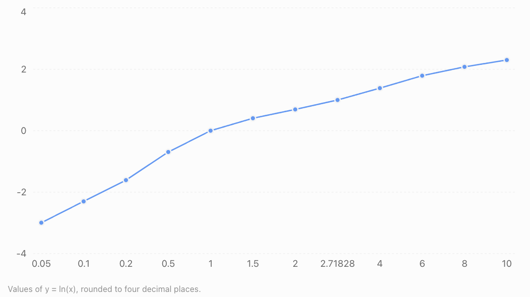
As x approaches zero from the right:
\[ \lim_{x\to0^+}\ln(x)=-\infty \]As x increases without bound:
\[ \lim_{x\to\infty}\ln(x)=\infty \]The function grows indefinitely, but very slowly.
Natural Logarithms and Inverse Functions
The natural logarithmic function and the natural exponential function are inverses.
This means that each function reverses the effect of the other.
The fundamental identities are:
\[ \boxed{\ln(e^x)=x} \]for every real x, and:
\[ \boxed{e^{\ln(x)}=x} \]for x > 0.
Reflection across y = x
Inverse functions have graphs that are reflections of each other across the line y = x.
For example:
-
The point (0, 1) on y = eˣ corresponds to (1, 0) on y = ln(x).
-
The point (1, e) on y = eˣ corresponds to (e, 1) on y = ln(x).
Inverse relationship between eˣ and ln(x)
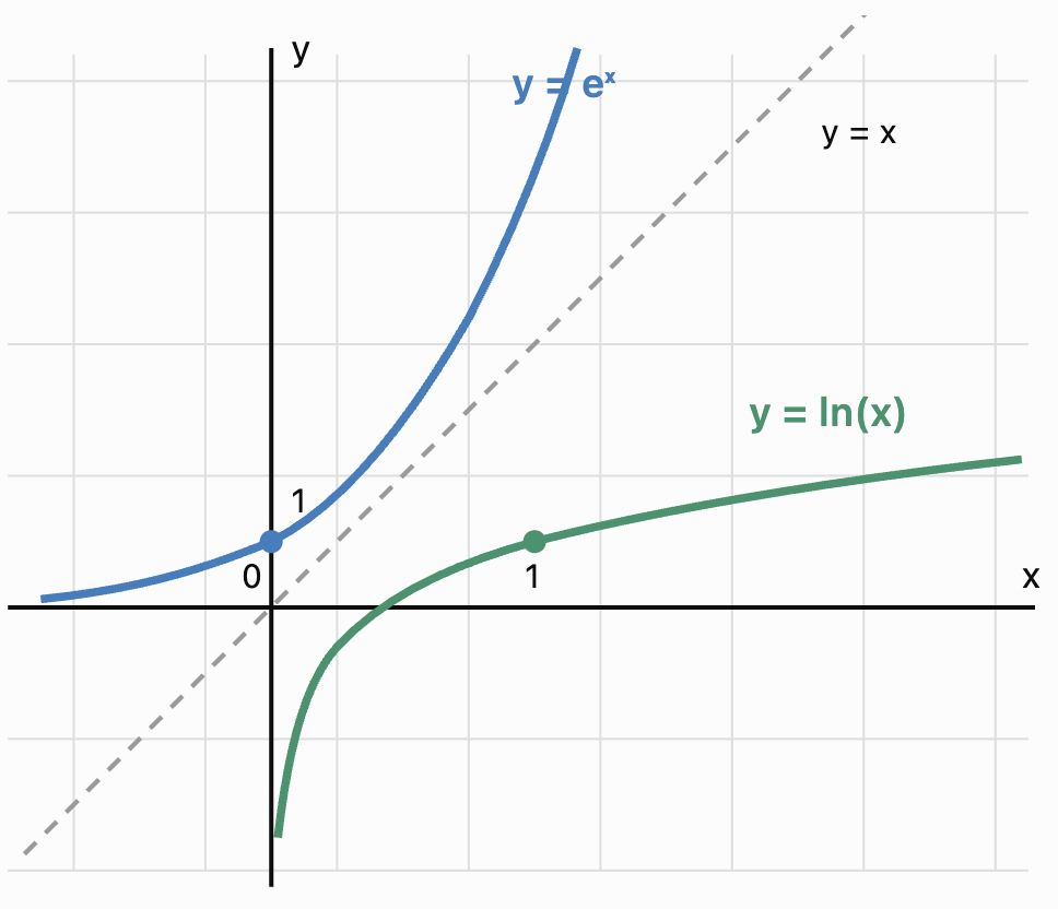 Conceptual illustration of the inverse relationship. The two curves are reflections across y = x; the drawing is schematic rather than a precision coordinate plot.
This inverse relationship is the foundation for solving natural exponential and logarithmic equations.
Properties of Natural Logarithms
Natural logarithms follow the same laws as logarithms with other valid bases.
These properties allow us to simplify expressions and solve equations.
For positive real numbers a and b, and any real number r:
Product property
\[ \boxed{\ln(ab)=\ln(a)+\ln(b)} \]The logarithm of a product equals the sum of the logarithms.
Example:
\[ \ln(2e)=\ln2+\ln e \]Since ln(e) = 1:
\[ \boxed{\ln(2e)=\ln2+1} \]Quotient property
\[ \boxed{\ln\left(\frac ab\right)=\ln(a)-\ln(b)} \]Example:
\[ \ln\left(\frac{e^3}{5}\right)=\ln(e^3)-\ln5 \]\[ \boxed{=3-\ln5} \]Power property
\[ \boxed{\ln(a^r)=r\ln(a)} \]Example:
\[ \ln(7^3)=3\ln7 \]Special identities
\[ \ln1=0 \]\[ \ln e=1 \]\[ \ln(e^x)=x \]\[ e^{\ln x}=x\quad(x>0) \]Worked Example 4: Expanding a Logarithm
Expand:
\[ \ln(5x^3) \]Assume x > 0.
Using the product property:
\[ \ln(5x^3)=\ln5+\ln(x^3) \]Apply the power property:
\[ \boxed{\ln(5x^3)=\ln5+3\ln x} \]Worked Example 5: Expanding a Quotient
Expand:
\[ \ln\left(\frac{3x^2}{y^4}\right) \]Assume x > 0 and y > 0.
Apply the quotient property:
\[ =\ln(3x^2)-\ln(y^4) \]Apply the product and power properties:
\[ \boxed{\ln3+2\ln x-4\ln y} \]For unrestricted nonzero real x and y, the fully general expression would instead use ln|x| and ln|y|.
Worked Example 6: Condensing Logarithms
Write as a single logarithm:
\[ 2\ln x+\ln3-\ln5 \]Assume x > 0.
Apply the power property:
\[ 2\ln x=\ln(x^2) \]Then combine:
\[ \ln(x^2)+\ln3=\ln(3x^2) \]Finally:
\[ \boxed{\ln\left(\frac{3x^2}{5}\right)} \]Solving Natural Logarithmic Equations
Natural logarithmic equations can be solved by converting between logarithmic and exponential forms.
The essential rule is:
\[ \ln(A)=b\iff A=e^b \]provided A > 0.
Worked Example 7: A Simple Logarithmic Equation
Solve:
\[ \ln x=3 \]Rewrite in exponential form:
\[ x=e^3 \]Therefore:
\[ \boxed{x\approx20.086} \]Worked Example 8: Logarithm of a Linear Expression
Solve:
\[ \ln(2x-1)=2 \]Step 1: Convert to exponential form.
\[ 2x-1=e^2 \]Step 2: Isolate x.
\[ 2x=e^2+1 \]\[ x=\frac{e^2+1}{2} \]Step 3: Evaluate.
\[ \boxed{x\approx4.195} \]Step 4: Check the domain.
The logarithm requires:
\[ 2x-1>0 \]\[ x>\frac12 \]Our solution satisfies the restriction.
Worked Example 9: Combining Logarithms
Solve:
\[ \ln x+\ln(x-3)=\ln10 \]Step 1: Identify domain restrictions.
\[ x>0,\qquad x-3>0 \]Therefore:
\[ x>3 \]Step 2: Combine the logarithms.
\[ \ln[x(x-3)]=\ln10 \]Step 3: Equate arguments.
\[ x(x-3)=10 \]\[ x^2-3x-10=0 \]Step 4: Factorise.
\[ (x-5)(x+2)=0 \]Therefore:
\[ x=5\quad\text{or}\quad x=-2 \]Step 5: Check the domain.
Since x > 3, the value −2 is invalid.
\[ \boxed{x=5} \]This illustrates why checking logarithmic domains is essential.
Solving Exponential Equations Using Natural Logarithms
Natural logarithms are also useful when the unknown appears in an exponent.
Worked Example 10: Solving an Exponential Equation
Solve:
\[ 5e^{0.4x}=30 \]Divide by 5:
\[ e^{0.4x}=6 \]Take natural logarithms:
\[ 0.4x=\ln6 \]Rearrange:
\[ x=\frac{\ln6}{0.4} \]\[ \boxed{x\approx4.479} \]Worked Example 11: Solving an Equation with a General Exponential Base
Solve:
\[ 3^x=20 \]Take natural logarithms of both sides:
\[ \ln(3^x)=\ln20 \]Apply the power property:
\[ x\ln3=\ln20 \]Therefore:
\[ x=\frac{\ln20}{\ln3} \]\[ \boxed{x\approx2.727} \]This method works with any positive exponential base other than 1.
Transformations of Natural Logarithmic Functions
The graph of y = ln(x) can be transformed through translations, reflections, and stretches.
A general form is:
\[ f(x)=a\ln[b(x-h)]+k \]where a and b are nonzero constants.
The parameters influence the graph's position and shape.
Function
Transformation
y = ln(x) + 3
Shift upward 3 units
y = ln(x − 2)
Shift right 2 units
y = ln(x + 4)
Shift left 4 units
y = −ln(x)
Reflection across the x-axis
y = 2ln(x)
Vertical stretch by factor 2
y = ln(−x)
Reflection across the y-axis
Worked Example 12: Analysing a Transformed Function
Consider:
\[ f(x)=2\ln(x-3)+1 \]Identify the domain, vertical asymptote, and transformations.
Transformations:
-
Shift right 3 units.
-
Vertical stretch by factor 2.
-
Shift upward 1 unit.
Domain:
The logarithm requires:
\[ x-3>0 \]\[ \boxed{x>3} \]Vertical asymptote:
\[ \boxed{x=3} \]Range:
All real numbers.
Finding the x-intercept
Set f(x) = 0.
\[ 2\ln(x-3)+1=0 \]\[ 2\ln(x-3)=-1 \]\[ \ln(x-3)=-\frac12 \]Convert to exponential form:
\[ x-3=e^{-1/2} \]\[ x=3+e^{-1/2} \]\[ \boxed{x\approx3.607} \]The graph crosses the x-axis at approximately (3.607, 0).
Natural Logarithms and Continuous Growth
One of the most important applications of natural logarithms is solving continuous growth and decay models.
The general model is:
\[ \boxed{Q(t)=Q_0e^{kt}} \]Where:
-
Q(t) = quantity at time t
-
Q₀ = initial quantity
-
k = continuous growth or decay rate
-
t = time
Natural logarithms allow us to solve for t when the initial and final quantities are known.
Starting with:
\[ Q=Q_0e^{kt} \]Divide by Q₀:
\[ \frac{Q}{Q_0}=e^{kt} \]Take natural logarithms:
\[ \ln\left(\frac{Q}{Q_0}\right)=kt \]Therefore:
\[ \boxed{t=\frac{\ln(Q/Q_0)}{k}} \]This formula is valid when Q and Q₀ are positive and k is nonzero.
Application: Population Growth
Worked Example 13: Time Required for Population Growth
A bacterial population initially contains 500 bacteria and grows continuously at 12% per hour.
How long will it take to reach 2,000 bacteria?
The model is:
\[ P(t)=500e^{0.12t} \]Set P(t) = 2000.
\[ 2000=500e^{0.12t} \]Divide by 500:
\[ 4=e^{0.12t} \]Take natural logarithms:
\[ \ln4=0.12t \]Rearrange:
\[ t=\frac{\ln4}{0.12} \]\[ t=\frac{1.386294}{0.12} \]\[ \boxed{t\approx11.55\text{ hours}} \]The population reaches 2,000 bacteria after approximately 11.55 hours under the model.
Application: Doubling Time
The doubling time is the time required for a growing quantity to become twice its initial value.
For:
\[ Q(t)=Q_0e^{kt} \]set:
\[ 2Q_0=Q_0e^{kt} \]Divide by Q₀:
\[ 2=e^{kt} \]Take natural logarithms:
\[ \ln2=kt \]Therefore:
\[ \boxed{t_d=\frac{\ln2}{k}} \]for k > 0.
Worked Example 14: Doubling Time
A population grows continuously at 5% per year.
Calculate its doubling time.
\[ t_d=\frac{\ln2}{0.05} \]\[ t_d=\frac{0.693147}{0.05} \]\[ \boxed{t_d\approx13.86\text{ years}} \]The population doubles approximately every 13.86 years if the continuous growth rate remains constant.
Application: Radioactive Decay
Natural logarithms are also essential for investigating radioactive decay.
The model is:
\[ N(t)=N_0e^{-\lambda t} \]Where λ is the positive decay constant.
Half-life formula
The half-life is the time required for the expected remaining quantity to decrease to half its original value.
\[ \boxed{t_{1/2}=\frac{\ln2}{\lambda}} \]Worked Example 15: Calculating Half-Life
A radioactive substance has a decay constant of 0.035 per year.
Calculate its half-life.
\[ t_{1/2}=\frac{\ln2}{0.035} \]\[ t_{1/2}=\frac{0.693147}{0.035} \]\[ \boxed{t_{1/2}\approx19.80\text{ years}} \]The substance has a half-life of approximately 19.8 years.
Application: Continuous Compound Interest
The continuous compound interest formula is:
\[ A=Pe^{rt} \]Where:
-
A = final amount
-
P = initial investment
-
r = annual interest rate
-
t = time in years
Natural logarithms allow us to calculate how long an investment needs to reach a target amount.
Worked Example 16: Investment Growth
An investment of $4,000 earns 6% annual interest compounded continuously.
How long will it take to reach $7,000?
Use:
\[ 7000=4000e^{0.06t} \]Divide by 4000:
\[ 1.75=e^{0.06t} \]Take natural logarithms:
\[ \ln1.75=0.06t \]Rearrange:
\[ t=\frac{\ln1.75}{0.06} \]\[ t=\frac{0.559616}{0.06} \]\[ \boxed{t\approx9.33\text{ years}} \]The investment reaches $7,000 after approximately 9.33 years.
Application: Natural Logarithms in Science
Natural logarithms appear in many scientific relationships.
Chemical Kinetics
First-order reactions can be analysed using logarithmic relationships. If concentration follows [A] = [A]₀e⁻ᵏᵗ, taking natural logarithms gives ln[A] = ln[A]₀ − kt.
Electrical Circuits
Capacitor discharge can be modelled exponentially. Natural logarithms help determine the time required for voltage to decrease to a specified level.
Biology
Natural logarithms help determine growth rates and doubling times for populations during approximately exponential growth phases.
Finance
Natural logarithms are used to calculate investment times, continuous rates of return, and other quantities in financial models.
Linearising Exponential Data
Natural logarithms can transform an exponential relationship into a linear relationship.
Suppose:
\[ y=Ae^{kx} \]where A > 0.
Take natural logarithms:
\[ \ln y=\ln(Ae^{kx}) \]Using logarithm properties:
\[ \ln y=\ln A+\ln(e^{kx}) \]Therefore:
\[ \boxed{\ln y=\ln A+kx} \]This is a straight-line equation in the variables x and ln
.
Its slope is k, and its intercept is ln(A).
Worked Example 17: Finding an Exponential Model
Suppose a quantity follows:
\[ y=Ae^{kx} \]and the data include:
-
At x = 0, y = 100.
-
At x = 4, y = 180.
Find A and k.
Step 1: Find A.
At x = 0:
\[ 100=Ae^0 \]\[ \boxed{A=100} \]Step 2: Substitute the second point.
\[ 180=100e^{4k} \]Divide by 100:
\[ 1.8=e^{4k} \]Take natural logarithms:
\[ \ln1.8=4k \]\[ k=\frac{\ln1.8}{4} \]\[ \boxed{k\approx0.14695} \]Therefore, the model is:
\[ \boxed{y=100e^{0.14695x}} \]The continuous growth rate is approximately 14.695% per unit of x.
This technique is useful in statistics because logarithmic transformations can reveal exponential patterns in data.
Common Mistakes
Mistake 1: Confusing ln(x) with log₁₀(x)
Natural logarithms use base e, while common logarithms use base 10.
Correction: Check which logarithm is required.
Mistake 2: Assuming ln(a + b) = ln(a) + ln(b)
This is false in general.
For example:
\[ \ln(2+3)=\ln5 \]but:
\[ \ln2+\ln3=\ln6 \]These are not equal.
Mistake 3: Taking the logarithm of zero or a negative number
The real-valued natural logarithm is defined only for positive inputs.
Correction: Check the domain before solving.
Mistake 4: Forgetting to check extraneous solutions
Algebraic manipulation may produce solutions that make a logarithm's argument zero or negative.
Correction: Substitute solutions into the original equation.
Mistake 5: Applying the power property incorrectly
The property is:
\[ \ln(x^n)=n\ln x \]for x > 0.
For even integer powers and negative x, absolute values may be required in the expanded expression.
Mistake 6: Confusing ln(eˣ) with eˡⁿ⁽ˣ⁾
Both inverse identities are useful, but the second requires x > 0.
Correction: Pay attention to domain restrictions.
Mistake 7: Using an incorrect growth-rate sign
A positive continuous rate represents growth, while a negative rate represents decay.
Correction: Interpret the sign of the exponent coefficient carefully.
Key Terms
-
Natural Logarithm: A logarithm with base e, written ln(x).
-
Euler's Number (e): An irrational constant approximately equal to 2.71828.
-
Logarithmic Function: A function involving the logarithm of a variable expression.
-
Inverse Function: A function that reverses the effect of another function.
-
Exponential Function: A function in which a variable appears in an exponent.
-
Domain: The set of allowable input values.
-
Range: The set of possible output values.
-
Vertical Asymptote: A vertical line approached by a graph as function values increase or decrease without bound.
-
Product Property: ln(ab) = ln(a) + ln(b).
-
Quotient Property: ln(a/b) = ln(a) − ln(b).
-
Power Property: ln(aʳ) = r ln(a), for a > 0.
-
Exponential Growth: Increase at a rate proportional to the current quantity.
-
Exponential Decay: Decrease at a rate proportional to the current quantity.
-
Continuous Growth Rate: The instantaneous relative growth rate in an exponential model.
-
Doubling Time: The time required for a growing quantity to double.
-
Half-Life: The time required for a decaying quantity to halve.
-
Continuous Compounding: The limiting form of increasingly frequent interest compounding.
-
Linearisation: Transforming a nonlinear relationship into a linear form.
-
Extraneous Solution: A solution produced during algebraic manipulation that does not satisfy the original equation.
Key Takeaways
-
Natural logarithms use base e and are written ln(x).
-
The natural logarithm is the inverse of the natural exponential function.
-
The identities ln(eˣ) = x and eˡⁿ⁽ˣ⁾ = x are fundamental.
-
The domain of ln(x) is x > 0, and its range is all real numbers.
-
The graph of y = ln(x) passes through (1, 0) and has a vertical asymptote at x = 0.
-
Natural logarithms follow product, quotient, and power properties.
-
Logarithmic equations must be solved with careful attention to domain restrictions.
-
Natural logarithms can solve equations where the unknown appears in an exponent.
-
Continuous growth and decay models can be rearranged using natural logarithms.
-
Doubling time and half-life formulas are derived using ln(2).
-
Natural logarithms are useful in finance, biology, chemistry, and physics.
-
Exponential relationships can be linearised by taking natural logarithms.
Check Your Understanding
Questions
Question 1: Exact Values
Evaluate:
a) ln(1)
b) ln(e⁴)
c) ln(e⁻²)
Question 2: Calculator Evaluation
Evaluate ln(12), correct to three decimal places.
Question 3: Expanding Logarithms
Expand:
\[ \ln(4x^3) \]Assume x > 0.
Question 4: Condensing Logarithms
Write as a single logarithm:
\[ 3\ln x+\ln2-\ln5 \]Assume x > 0.
Question 5: Solving a Simple Equation
Solve:
\[ \ln x=4 \]Question 6: Solving a Linear Logarithmic Equation
Solve:
\[ \ln(3x+2)=2 \]Question 7: Combining Logarithms
Solve:
\[ \ln x+\ln(x-2)=\ln8 \]Question 8: Exponential Equations
Solve:
\[ 4e^{0.5x}=20 \]Question 9: General Exponential Equations
Solve:
\[ 5^x=40 \]Question 10: Transformations
For:
\[ f(x)=\ln(x-4)+2 \]state the domain, vertical asymptote, and transformations relative to y = ln(x).
Question 11: Continuous Growth
A population starts at 600 and grows continuously at 9% per year.
How long will it take to reach 1,200?
Question 12: Continuous Interest
An investment of $5,000 earns 4% annual interest compounded continuously.
How long will it take to reach $8,000?
Question 13: Half-Life
A radioactive substance has a decay constant of 0.06 per day.
Calculate its half-life.
Question 14: Exponential Modelling
A quantity follows:
\[ y=Ae^{kx} \]Given that y = 50 when x = 0 and y = 100 when x = 5, determine A and k.
Fully Worked Answers
Answer 1: Exact Values
a)
\[ \boxed{\ln1=0} \]b)
\[ \boxed{\ln(e^4)=4} \]c)
\[ \boxed{\ln(e^{-2})=-2} \]Answer 2: Calculator Evaluation
\[ \ln12\approx2.48490665 \]To three decimal places:
\[ \boxed{2.485} \]Answer 3: Expanding Logarithms
\[ \ln(4x^3) \]Apply the product property:
\[ =\ln4+\ln(x^3) \]Apply the power property:
\[ \boxed{\ln4+3\ln x} \]Answer 4: Condensing Logarithms
\[ 3\ln x+\ln2-\ln5 \]Apply the power property:
\[ =\ln(x^3)+\ln2-\ln5 \]Combine:
\[ =\ln(2x^3)-\ln5 \]Therefore:
\[ \boxed{\ln\left(\frac{2x^3}{5}\right)} \]Answer 5: Solving a Simple Equation
\[ \ln x=4 \]Convert to exponential form:
\[ x=e^4 \]\[ \boxed{x\approx54.598} \]Answer 6: Solving a Linear Logarithmic Equation
\[ \ln(3x+2)=2 \]Convert to exponential form:
\[ 3x+2=e^2 \]Rearrange:
\[ 3x=e^2-2 \]\[ x=\frac{e^2-2}{3} \]\[ \boxed{x\approx1.796} \]The solution satisfies the domain condition 3x + 2 > 0.
Answer 7: Combining Logarithms
\[ \ln x+\ln(x-2)=\ln8 \]Domain restriction:
\[ x>2 \]Combine logarithms:
\[ \ln[x(x-2)]=\ln8 \]Equate arguments:
\[ x(x-2)=8 \]\[ x^2-2x-8=0 \]Factorise:
\[ (x-4)(x+2)=0 \]Therefore:
\[ x=4\quad\text{or}\quad x=-2 \]Only x = 4 satisfies x > 2.
\[ \boxed{x=4} \]Answer 8: Exponential Equations
\[ 4e^{0.5x}=20 \]Divide by 4:
\[ e^{0.5x}=5 \]Take natural logarithms:
\[ 0.5x=\ln5 \]\[ x=\frac{\ln5}{0.5} \]\[ \boxed{x\approx3.219} \]Answer 9: General Exponential Equations
\[ 5^x=40 \]Take natural logarithms:
\[ x\ln5=\ln40 \]\[ x=\frac{\ln40}{\ln5} \]\[ \boxed{x\approx2.292} \]Answer 10: Transformations
\[ f(x)=\ln(x-4)+2 \]The graph is shifted:
-
Right 4 units.
-
Upward 2 units.
The domain requires:
\[ x-4>0 \]\[ \boxed{x>4} \]The vertical asymptote is:
\[ \boxed{x=4} \]Answer 11: Continuous Growth
The model is:
\[ P(t)=600e^{0.09t} \]Set P(t) = 1200.
\[ 1200=600e^{0.09t} \]Divide by 600:
\[ 2=e^{0.09t} \]Take natural logarithms:
\[ \ln2=0.09t \]\[ t=\frac{\ln2}{0.09} \]\[ \boxed{t\approx7.70\text{ years}} \]Answer 12: Continuous Interest
\[ A=Pe^{rt} \]Substitute:
\[ 8000=5000e^{0.04t} \]Divide by 5000:
\[ 1.6=e^{0.04t} \]Take natural logarithms:
\[ \ln1.6=0.04t \]\[ t=\frac{\ln1.6}{0.04} \]\[ \boxed{t\approx11.75\text{ years}} \]Answer 13: Half-Life
Use:
\[ t_{1/2}=\frac{\ln2}{\lambda} \]Substitute λ = 0.06.
\[ t_{1/2}=\frac{0.693147}{0.06} \]\[ \boxed{t_{1/2}\approx11.55\text{ days}} \]Answer 14: Exponential Modelling
Given:
\[ y=Ae^{kx} \]At x = 0, y = 50.
\[ 50=Ae^0 \]\[ \boxed{A=50} \]At x = 5, y = 100.
\[ 100=50e^{5k} \]Divide by 50:
\[ 2=e^{5k} \]Take natural logarithms:
\[ \ln2=5k \]\[ k=\frac{\ln2}{5} \]\[ \boxed{k\approx0.1386} \]Therefore, the model is:
\[ \boxed{y=50e^{0.1386x}} \]The continuous growth rate is approximately 13.86% per unit of x.
Final Reflection
Natural logarithms are essential mathematical tools because they allow us to reverse exponential relationships.
They provide methods for solving equations, interpreting logarithmic graphs, simplifying expressions, and analysing processes that involve continuous growth or decay.
Their usefulness extends far beyond algebra. Natural logarithms help determine investment times, population doubling times, radioactive half-lives, and many other quantities in scientific and economic models.
The central relationship to remember is that natural logarithms and natural exponential functions are inverses:
\[ \boxed{\ln(e^x)=x} \]and:
\[ \boxed{e^{\ln x}=x\qquad(x>0)} \]Understanding these relationships provides a strong foundation for advanced algebra, calculus, statistics, and mathematical modelling.
-
3. Continuous Growth and Decay
Learning outcomes
- I can model continuously compounded growth.
- I can model continuous decay.
- I can compare discrete and continuous models.
- I can interpret continuous growth models.
- I can solve authentic applications.
Introduction
Imagine investing money in a savings account that earns interest continuously. As the account balance grows, the amount of interest earned also increases because interest is calculated on an increasingly large balance.
Now imagine a radioactive substance gradually losing mass as its unstable nuclei decay. The amount that decays during a particular interval depends on how much radioactive material remains.
Although these situations appear different, they can be described using the same mathematical principle: the rate of change of a quantity is proportional to the quantity currently present.
This principle leads to continuous exponential growth and decay models.
These models are used in finance, population biology, medicine, chemistry, physics, and environmental science. They allow us to predict future quantities, calculate doubling times and half-lives, compare different growth processes, and solve practical problems involving time and rates of change.
Understanding Continuous Growth and Decay
A quantity experiences continuous exponential growth when its instantaneous rate of increase is proportional to its current value.
A quantity experiences continuous exponential decay when its instantaneous rate of decrease is proportional to its current value.
Both processes can be represented by:
Where:
-
Q(t) = quantity at time t
-
Q₀ = initial quantity
-
e = Euler's number, approximately 2.71828
-
k = continuous growth or decay constant
-
t = elapsed time
The sign of k determines the behaviour.
|
Value of k |
Behaviour |
|---|---|
|
k > 0 |
Exponential growth |
|
k = 0 |
Constant quantity |
|
k < 0 |
Exponential decay |
The units of k are the reciprocal of the time unit. For example, if t is measured in years, k is measured per year.
Why is the model called continuous?
In a continuous model, the quantity changes throughout time rather than only at separate intervals.
The underlying mathematical relationship is:
This means that the instantaneous rate of change is proportional to the current quantity.
For example, if a population contains twice as many organisms, its instantaneous growth rate is twice as large, provided k remains constant.
Visualising Continuous Growth and Decay
Consider two quantities, both initially equal to 100.
One grows with k = 0.25, while the other decays with k = −0.25.
Their models are:
Growth: Q(t) = 100e^(0.25t)
Decay: Q(t) = 100e^(−0.25t)
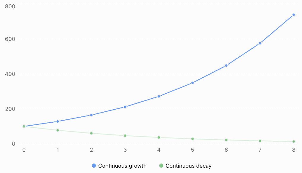
Notice that:
-
Both quantities begin at 100.
-
The growing quantity increases by larger absolute amounts over successive equal time intervals.
-
The decaying quantity decreases, but its absolute losses become smaller.
-
The decay model approaches zero without reaching it in finite time.
-
Both processes have a constant proportional rate of change, even though their absolute rates change.
The constant proportional rate is the defining feature of exponential growth and decay.
Developing Continuous Growth Models
Suppose a population initially contains 500 organisms and grows continuously at a rate of 8% per year.
The initial quantity is:
Q₀ = 500
The continuous growth constant is:
k = 0.08 per year
Therefore:
Worked Example 1: Predicting Population Growth
Estimate the population after 6 years.
Step 1: Write the model.
Step 2: Substitute t = 6.
Step 3: Evaluate.
The predicted population after six years is approximately 808 organisms.
Interpreting the result
The population has increased from 500 to approximately 808.
The absolute increase is:
808 − 500 = 308 organisms.
The continuous growth constant remains 0.08 per year, but the population's instantaneous absolute growth rate increases as the population becomes larger.
This distinction between proportional growth and absolute growth is important.
Continuously Compounded Interest
One of the best-known applications of continuous exponential growth is compound interest.
With ordinary compound interest, interest is added at specified intervals, such as annually, monthly, or daily.
With continuous compounding, we consider the limiting situation as the compounding frequency increases without bound.
The continuously compounded interest formula is:
Where:
-
A = final account balance
-
P = principal, or initial investment
-
r = nominal annual interest rate expressed as a decimal
-
t = time in years
Explore continuous compound interest
Change the initial investment, annual interest rate, or investment period to explore how continuous compounding affects the final balance.Worked Example 2: Continuous Compound Interest
An investment of $6,000 earns interest at a nominal annual rate of 4.5%, compounded continuously.
Calculate the value after 8 years.
Step 1: Identify the values.
P = 6000
r = 0.045
t = 8
Step 2: Substitute.
Step 3: Evaluate.
Step 4: Calculate the interest earned.
The investment earns approximately $2,599.98 in interest over eight years, assuming the rate remains constant and there are no deposits, withdrawals, taxes, or fees.
Continuous Exponential Decay
Exponential decay occurs when a quantity decreases at a rate proportional to the amount remaining.
A convenient decay model is:
Where λ is a positive decay constant.
This is equivalent to the general model Q(t) = Q₀eᵏᵗ with k = −λ.
Examples include:
-
Radioactive decay.
-
Certain chemical reactions.
-
Drug elimination under first-order conditions.
-
Capacitor discharge.
-
Temperature differences during Newtonian cooling.
Worked Example 3: Decaying Substance
A substance initially has a mass of 400 g and decays continuously at a rate of 12% per hour.
Calculate its remaining mass after 5 hours.
Step 1: Write the model.
Step 2: Substitute t = 5.
Step 3: Evaluate.
Step 4: Calculate the mass lost.
Approximately 180.48 g has been lost.
The mass remaining is always positive in this idealised model.
Comparing Discrete and Continuous Growth
Exponential growth can be modelled using discrete or continuous approaches.
Discrete growth
Discrete growth uses a constant multiplier over each complete time period.
The model is:
Where:
-
Q₀ = initial quantity
-
r = effective growth rate per period
-
n = number of periods
For example, if a population grows by exactly 5% each year:
Continuous growth
Continuous growth uses the natural exponential function:
Here, k is the continuous relative growth rate.
Although these models look different, they can describe the same values at whole-number times.
Converting between growth rates
The relationship is:
Therefore:
and:
These formulas are essential for comparing discrete and continuous growth rates.
Worked Example 4: Converting a Discrete Rate to a Continuous Rate
A population increases by exactly 6% each year.
Find the equivalent continuous growth rate.
The annual growth multiplier is:
Therefore:
The equivalent continuous growth rate is approximately 5.827% per year.
The models:
Q = Q₀(1.06)ⁿ
and
Q(t) = Q₀e^(0.05827t)
produce the same quantities at integer-year times, apart from rounding.
Worked Example 5: Converting a Continuous Rate to an Effective Annual Rate
An investment grows continuously at 8% per year.
Find its effective annual growth rate.
A continuous rate of 8% per year corresponds to an effective annual increase of approximately 8.329%.
It is not exactly an 8% annual increase.
Comparing Compounding Frequencies
For a nominal annual interest rate r compounded m times per year:
As m becomes increasingly large, the expression approaches continuous compounding.
Consider $1,000 invested at a nominal annual interest rate of 10% for one year.
|
Compounding frequency |
Final amount |
|---|---|
|
Annually |
$1,100.00 |
|
Semiannually |
$1,102.50 |
|
Quarterly |
$1,103.81 |
|
Monthly |
$1,104.71 |
|
Daily (365 times) |
$1,105.16 |
|
Continuously |
$1,105.17 |
More frequent compounding produces a larger balance when the nominal rate is positive.
However, the additional benefit becomes smaller as the frequency increases.
The chart compares interest earned rather than total balances, making the relatively small differences easier to see.
Comparing Discrete and Continuous Decay
Discrete decay uses a constant percentage reduction during each time period.
For a fractional decay rate d per period:
where 0 < d < 1.
Continuous decay uses:
The equivalent rates satisfy:
Therefore:
Worked Example 6: Converting a Decay Rate
A substance loses exactly 15% of its mass each day.
Find the equivalent continuous decay constant.
The daily remaining fraction is:
Therefore:
The corresponding continuous decay model is:
This model matches the discrete model at whole-day times, subject to rounding.
The continuous decay constant is approximately 0.16252 per day, not 0.15 per day.
Interpreting Continuous Growth Models
A continuous exponential model provides more information than simply the predicted quantity.
Consider:
where t is measured in years.
We can interpret its components.
Initial quantity
At t = 0:
The initial population is 2,500.
Continuous growth rate
The constant k = 0.035 indicates a continuous relative growth rate of 3.5% per year.
Instantaneous rate of change
Differentiate the model:
Therefore:
At t = 0:
The population is initially increasing at an instantaneous rate of 87.5 organisms per year.
When the population reaches 4,000:
Its instantaneous growth rate becomes 140 organisms per year.
The relative growth rate remains constant, but the absolute growth rate increases.
Instantaneous rate versus average rate
The instantaneous rate describes how quickly the quantity is changing at a particular moment.
The average rate of change over an interval is:
These are generally different for exponential functions.
This distinction is especially important in calculus and mathematical modelling.
Doubling Time
The doubling time is the time required for a continuously growing quantity to become twice its initial value.
Starting with:
At doubling:
Divide by Q₀:
Take natural logarithms:
Therefore:
where k > 0.
Worked Example 7: Calculating Doubling Time
A population grows continuously at 4.5% per year.
Calculate its doubling time.
The population doubles approximately every 15.4 years if the growth constant remains unchanged.
Notice that doubling time does not depend on the initial population.
A population of 500 and a population of 50,000 have the same doubling time when they share the same constant k.
Half-Life
The half-life is the time required for an exponentially decaying quantity to decrease to half its initial value.
For:
the half-life is:
where λ > 0.
Worked Example 8: Radioactive Half-Life
A radioactive substance has a decay constant of 0.075 per year.
Calculate its half-life.
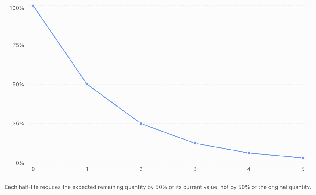
After approximately 9.24 years, half the original radioactive nuclei are expected to remain.
After two half-lives, one-quarter remain.
After three half-lives, one-eighth remain.
Exponential decay over successive half-lives
Finding the Growth or Decay Constant from Data
Sometimes the initial and final quantities are known, but the growth or decay constant is unknown.
Start with:
Divide by Q₀:
Take natural logarithms:
Rearrange:
This formula allows us to determine the continuous rate from observations.
Worked Example 9: Finding a Growth Constant
A population increases from 800 to 1,200 over five years.
Assuming continuous exponential growth, calculate k.
The continuous growth rate is approximately 8.109% per year.
The model becomes:
Worked Example 10: Finding a Decay Constant
A substance decreases from 300 g to 180 g over four hours.
Find its continuous decay constant.
The signed growth constant is −0.12771 per hour.
Equivalently, the positive decay constant is:
The model is:
Solving Authentic Applications
Continuous exponential models become particularly useful when the unknown is time, a growth rate, or an initial quantity.
Application 1: Medicine — Drug Elimination
A medication has an initial amount of 200 mg in the body.
Under an idealised first-order elimination model, the amount remaining is:
where t is measured in hours.
How long will it take for the amount to decrease to 50 mg?
Step 1: Substitute the target amount.
Step 2: Divide by 200.
Step 3: Take natural logarithms.
Step 4: Solve.
The model predicts that the amount decreases to 50 mg after approximately 7.70 hours.
Actual drug elimination depends on the medication, individual physiology, and whether first-order kinetics apply. This calculation is a mathematical illustration, not a dosing recommendation.
Application 2: Finance — Reaching a Savings Goal
An investor deposits $10,000 into an account earning 5% nominal annual interest compounded continuously.
How long will it take for the account to reach $15,000?
Divide by 10,000:
Take natural logarithms:
The investment reaches $15,000 after approximately 8.11 years under the assumed constant rate.
Application 3: Environmental Science — Pollutant Removal
A pollutant has an initial concentration of 80 mg/L.
Its concentration decreases continuously according to:
where t is measured in days.
Determine when the concentration falls to 10 mg/L.
The model predicts that the concentration reaches 10 mg/L after approximately 6.93 days.
This assumes a constant proportional removal rate, with no additional pollutant entering the system.
Application 4: Physics — Newton's Law of Cooling
A hot object cools in a room maintained at a constant temperature.
Under suitable conditions, Newton's law of cooling gives:
Where:
-
T(t) = temperature at time t
-
Tₐ = ambient temperature
-
T₀ = initial object temperature
-
k = positive cooling constant
Suppose a cup of coffee begins at 90°C in a room at 22°C, with k = 0.12 per minute.
Find its temperature after 10 minutes.
The coffee is predicted to cool to approximately 42.5°C.
Notice that the temperature difference from the surroundings, rather than the absolute temperature, follows an exponential decay model.
Evaluating Model Assumptions and Limitations
Continuous exponential models are useful, but they depend on important assumptions.
Constant proportional rate
The model assumes that k remains constant.
Real population growth may slow because of limited resources.
Investment rates may change over time.
Drug elimination may not always follow first-order kinetics.
Appropriate time interval
An exponential model may work well over a short period but become unrealistic over a much longer period.
For example, a bacterial population cannot grow exponentially forever in a closed container.
No unmodelled additions or removals
A simple decay model assumes the quantity is not replenished.
If additional pollutants enter a river, a basic exponential decay model may no longer describe the situation adequately.
Reliable measurements
Estimated growth and decay constants depend on the quality of the data.
Measurement error, missing observations, and inappropriate assumptions can produce misleading predictions.
Discrete versus continuous reality
Some processes occur through individual events but can still be modelled using continuous equations.
For example, radioactive nuclei decay individually, but the expected number remaining in a large sample follows an exponential law.
A continuous model is a mathematical description of the overall behaviour, not necessarily a claim that every underlying event occurs continuously.
Common Mistakes
Mistake 1: Confusing continuous and effective growth rates
A continuous growth rate of 5% does not mean exactly 5% growth over one year.
Correction: Use r = eᵏ − 1 to calculate the effective growth rate over one time unit.
Mistake 2: Using the wrong sign for decay
The expression Q = Q₀e⁰·¹ᵗ represents growth, not decay.
Correction: Use a negative exponent coefficient for decay.
Mistake 3: Mixing time units
A decay constant measured per hour cannot be used directly with time measured in days.
Correction: Convert time units before substituting.
Mistake 4: Treating half-life as a constant absolute decrease
After each half-life, half the current amount remains.
Correction: Apply a multiplicative factor of 0.5, not a fixed subtraction.
Mistake 5: Confusing continuous compounding with monthly compounding
These are different models.
Correction: Use A = Peʳᵗ for continuous compounding and A = P(1 + r/m)ᵐᵗ for m compounding periods per year.
Mistake 6: Forgetting logarithms when solving for time
When the unknown appears in the exponent, ordinary linear rearrangement is insufficient.
Correction: Isolate the exponential expression and take natural logarithms.
Mistake 7: Applying exponential models indefinitely
Many real processes change behaviour as conditions change.
Correction: Consider whether the model's assumptions remain valid over the prediction period.
Key Terms
-
Continuous Growth: Growth in which the instantaneous rate of increase is proportional to the current quantity.
-
Continuous Decay: Decrease in which the instantaneous rate of decrease is proportional to the current quantity.
-
Euler's Number (e): An irrational constant approximately equal to 2.71828.
-
Initial Quantity: The amount present at time zero.
-
Growth Constant: The positive parameter k in an exponential growth model.
-
Decay Constant: The positive parameter λ in an exponential decay model.
-
Continuous Compounding: The limiting form of compound interest as compounding frequency increases without bound.
-
Discrete Growth: Growth represented using fixed percentage changes over separate time periods.
-
Effective Growth Rate: The actual proportional increase over a specified time interval.
-
Instantaneous Rate of Change: The rate at which a quantity changes at a particular moment.
-
Relative Growth Rate: The instantaneous rate of change divided by the current quantity.
-
Doubling Time: The time required for an exponentially growing quantity to double.
-
Half-Life: The time required for an exponentially decaying quantity to halve.
-
Natural Logarithm: A logarithm with base e, written ln(x).
-
Exponential Model: A mathematical relationship in which a variable appears in an exponent.
-
First-Order Decay: A process in which the rate of decrease is proportional to the amount remaining.
-
Mathematical Assumption: A condition required for a model or method to be appropriate.
-
Extrapolation: Using a model to predict beyond the range of observed data.
Key Takeaways
-
Continuous growth and decay are modelled using Q(t) = Q₀eᵏᵗ.
-
Positive k represents growth; negative k represents decay.
-
Continuous compounding is modelled by A = Peʳᵗ.
-
Discrete growth uses Qₙ = Q₀(1 + r)ⁿ.
-
The equivalent discrete and continuous rates satisfy k = ln(1 + r).
-
Continuous decay can be written as Q(t) = Q₀e⁻λᵗ.
-
The equivalent discrete decay fraction satisfies λ = −ln(1 − d).
-
The instantaneous rate of change is proportional to the current quantity.
-
Doubling time is ln(2)/k for positive k.
-
Half-life is ln(2)/λ for positive λ.
-
Natural logarithms allow us to solve for time and growth constants.
-
Continuous exponential models are useful in finance, biology, medicine, chemistry, physics, and environmental science.
-
All predictions should be interpreted in the context of the model's assumptions and limitations.
Check Your Understanding
Questions
Question 1: Identifying Growth and Decay
Determine whether each model represents growth or decay.
a) Q(t) = 500e^(0.06t)
b) Q(t) = 800e^(−0.09t)
c) Q(t) = 200e^(0t)
Question 2: Continuous Population Growth
A population initially contains 1,500 organisms and grows continuously at 4% per year.
Write a model and calculate the population after 8 years.
Question 3: Continuous Compound Interest
An investment of $7,500 earns 5% annual interest compounded continuously.
Calculate its value after 12 years.
Question 4: Continuous Decay
A substance initially has a mass of 600 g and decays continuously at a rate of 8% per hour.
Calculate the remaining mass after 7 hours.
Question 5: Discrete to Continuous Growth
A population increases by exactly 7% annually.
Find the equivalent continuous growth constant.
Question 6: Continuous to Discrete Growth
An investment grows continuously at 6% per year.
Calculate its effective annual growth rate.
Question 7: Doubling Time
A population grows continuously at 3% per year.
Calculate its doubling time.
Question 8: Half-Life
A substance has a decay constant of 0.11 per day.
Calculate its half-life.
Question 9: Finding a Growth Constant
A population increases from 2,000 to 3,000 over 6 years.
Assuming continuous exponential growth, calculate the growth constant.
Question 10: Finding Time
A substance decays according to:
How long will it take for the mass to decrease to 125 g?
Question 11: Comparing Models
Explain the difference between:
Q(t) = 1000(1.05)ᵗ
and
Q(t) = 1000e^(0.05t).
Do they represent the same growth rate?
Question 12: Authentic Application
A lake contains a pollutant at a concentration of 120 mg/L. Its concentration decreases continuously at 18% per day.
Write a model and calculate when the concentration reaches 30 mg/L.
Question 13: Interpreting a Model
Consider:
Explain the meaning of 4000 and 0.025. Calculate the instantaneous growth rate when the population is 6,000.
Question 14: Evaluating Model Limitations
A scientist models a bacterial population using exponential growth and predicts that it will increase indefinitely.
Explain two reasons why this prediction may eventually become unrealistic.
Fully Worked Answers
Answer 1: Identifying Growth and Decay
a) k = 0.06, which is positive.
Exponential growth.
b) k = −0.09, which is negative.
Exponential decay.
c) k = 0.
The quantity remains constant at 200.
Answer 2: Continuous Population Growth
The model is:
After 8 years:
The predicted population is approximately 2,066 organisms.
Answer 3: Continuous Compound Interest
Use:
Substitute:
Answer 4: Continuous Decay
After 7 hours:
Answer 5: Discrete to Continuous Growth
The annual growth rate is r = 0.07.
The equivalent continuous growth rate is approximately 6.766% per year.
Answer 6: Continuous to Discrete Growth
Given k = 0.06:
The effective annual growth rate is approximately 6.184%.
Answer 7: Doubling Time
Answer 8: Half-Life
Answer 9: Finding a Growth Constant
Substitute:
The continuous growth rate is approximately 6.758% per year.
Answer 10: Finding Time
Divide by 500:
Take natural logarithms:
Rearrange:
The mass decreases to 125 g after approximately 17.33 time units.
Answer 11: Comparing Models
The first model:
represents an effective growth rate of exactly 5% per unit of time.
The second model:
represents a continuous growth rate of 5% per unit of time.
Its effective growth rate over one time unit is:
or approximately 5.127%.
Therefore, the models do not have exactly the same growth rate.
Answer 12: Authentic Application
The initial concentration is 120 mg/L.
The continuous decay constant is 0.18 per day.
The model is:
Set C(t) = 30.
Take natural logarithms:
The concentration reaches 30 mg/L after approximately 7.70 days.
Answer 13: Interpreting a Model
The model is:
The initial population is 4,000.
The continuous growth constant is 0.025, representing a continuous growth rate of 2.5% per time unit.
The instantaneous rate of change is:
When P = 6000:
The population is increasing at an instantaneous rate of 150 organisms per time unit.
Answer 14: Evaluating Model Limitations
Exponential population growth assumes that the relative growth rate remains constant.
This may become unrealistic because:
Limited resources: Nutrients, water, oxygen, or space may become insufficient to support continued growth.
Environmental changes: Waste accumulation, competition, disease, or temperature changes may reduce the growth rate.
A logistic growth model or another model incorporating environmental limits may become more appropriate.
Final Reflection
Continuous growth and decay models provide a powerful connection between exponential functions, natural logarithms, and real-world change.
Their central principle is that the instantaneous rate of change is proportional to the quantity currently present.
This allows us to model investments, populations, radioactive substances, chemical concentrations, and many other processes.
The most important general equation is:
Understanding how to interpret its parameters, compare it with discrete models, and solve for unknown quantities makes continuous exponential modelling a valuable tool across mathematics and science.
A successful mathematical model does more than produce an answer. It provides a meaningful interpretation of a real situation while recognising the assumptions and limitations on which the prediction depends.
4. Logistic Growth Models
Learning outcomes
- I can explain logistic growth.
- I can distinguish logistic and exponential growth.
- I can interpret carrying capacity.
- I can analyse logistic graphs.
- I can model real-world population growth.
Introduction
Imagine introducing a small population of rabbits into a large grassland. At first, food is plentiful, space is available, and the rabbits reproduce rapidly. As the population increases, however, more rabbits compete for the same resources.
Eventually, the population may become so large that the environment cannot support continued rapid growth.
This situation illustrates an important limitation of exponential growth: real populations cannot usually grow exponentially forever.
Exponential models assume that a population maintains a constant proportional growth rate. In reality, populations are influenced by food availability, water, space, competition, disease, and other environmental factors.
A logistic growth model accounts for these limitations by allowing population growth to slow as the population approaches the maximum level that the environment can sustain.
Logistic models produce a characteristic S-shaped curve and are widely used in ecology, population biology, epidemiology, resource management, and mathematical modelling.
In this lesson, we will explore the mathematical structure of logistic growth, compare it with exponential growth, interpret carrying capacity, analyse logistic graphs, and develop models for real-world populations.
What Is Logistic Growth?
Logistic growth is a pattern of population change in which growth is initially approximately exponential but gradually slows as the population approaches a limiting value.
This limiting value is called the carrying capacity.
Logistic growth typically occurs in three stages.
-
Early growth: The population is relatively small, resources are abundant, and growth accelerates.
-
Rapid growth: The population increases quickly, but competition for resources becomes increasingly important.
-
Slowing growth: Population growth decreases as the population approaches carrying capacity.
For an initial population below carrying capacity, the resulting graph is often S-shaped, also called a sigmoid curve.
The characteristic logistic growth curve
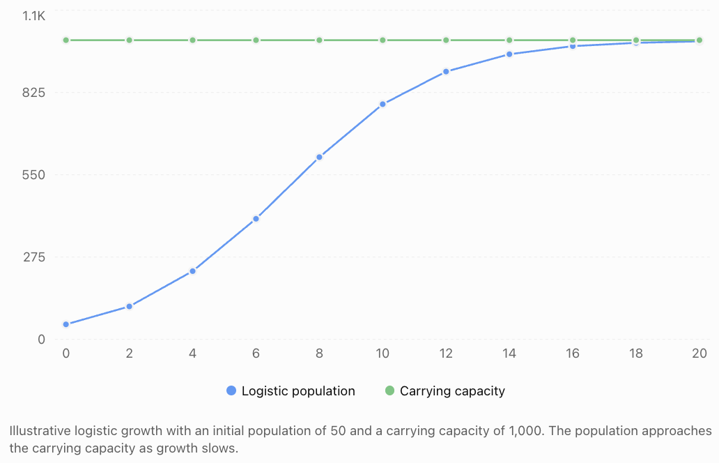
The population does not suddenly stop growing when it reaches a particular size. Instead, its growth rate gradually decreases as it approaches the limiting value.
Exponential Growth Versus Logistic Growth
Both exponential and logistic models describe population growth, but they make different assumptions.
Exponential growth
The exponential growth model is:
P(t) = P₀eʳᵗ
Where:
-
P(t) = population at time t
-
P₀ = initial population
-
r = constant continuous relative growth rate
-
t = time
The model assumes that the population's relative growth rate remains constant.
Consequently, the population grows without bound when r > 0.
Logistic growth
The logistic model modifies exponential growth by accounting for limited resources.
Its relative growth rate decreases as the population approaches carrying capacity.
|
Feature |
Exponential growth |
Logistic growth |
|---|---|---|
|
Graph shape |
J-shaped |
Usually S-shaped |
|
Resource availability |
Assumed unlimited or nonlimiting |
Limited |
|
Relative growth rate |
Constant |
Decreases as population increases |
|
Carrying capacity |
Not included |
Included |
|
Long-term behaviour |
Unlimited growth for r > 0 |
Approaches a limiting population |
|
Typical application |
Early population growth |
Growth under resource constraints |
Comparing the two models
Consider a population that begins with 50 organisms.
Suppose the exponential model has a continuous growth rate of 40% per year, while the logistic model has the same intrinsic growth parameter and a carrying capacity of 1,000.
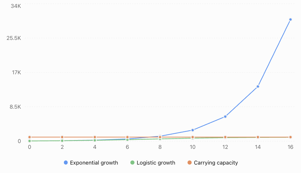
Initially, the models produce relatively similar predictions because the population is small compared with carrying capacity.
Over time, however, the exponential model continues increasing rapidly while the logistic model begins to level off.
The central difference is that logistic growth incorporates density-dependent limitations on population growth.
Carrying Capacity
The carrying capacity, represented by K, is the population size that an environment can sustain in the long term under the conditions assumed by the model.
Carrying capacity depends on factors such as:
-
Food availability.
-
Water availability.
-
Living space.
-
Competition.
-
Disease and predation.
-
Availability of shelter.
-
Environmental conditions.
For example, a lake may support approximately 5,000 fish under a particular set of ecological conditions.
If the population is much smaller than 5,000, resources may be plentiful and the population may increase.
As the population approaches 5,000, competition becomes stronger and population growth slows.
If the population temporarily exceeds carrying capacity, the logistic model predicts a decrease toward K.
Is carrying capacity always constant?
No.
In a basic logistic model, K is assumed to remain constant.
In real ecosystems, carrying capacity may change because of droughts, climate changes, habitat destruction, seasonal conditions, or changes in food availability.
Therefore, carrying capacity should be understood as a model parameter representing environmental limits under particular conditions, not necessarily a permanent population maximum.
The Logistic Growth Equation
The logistic growth model can be expressed as a differential equation.
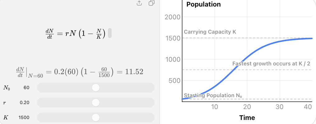
Where:
-
N = population size.
-
t = time.
-
r = intrinsic per-capita growth rate.
-
K = carrying capacity.
-
dN/dt = instantaneous rate of population change.
The expression (1 − N/K) is called the density-dependent limiting factor.
It reduces the growth rate as the population approaches carrying capacity.
Understanding the limiting factor
Suppose K = 1,000.
|
Population N |
N/K |
1 − N/K |
Interpretation |
|---|---|---|---|
|
100 |
0.10 |
0.90 |
Growth is only slightly reduced |
|
250 |
0.25 |
0.75 |
Some resource limitation |
|
500 |
0.50 |
0.50 |
Stronger limitation |
|
750 |
0.75 |
0.25 |
Growth is considerably reduced |
|
900 |
0.90 |
0.10 |
Growth is slow |
|
1,000 |
1.00 |
0 |
No net growth |
|
1,100 |
1.10 |
−0.10 |
Population decreases |
This table illustrates why logistic growth differs from exponential growth.
The population's instantaneous growth rate depends on both its current size and its proximity to carrying capacity.
The Logistic Population Function
The differential equation has a solution of the form:
Where:
-
P(t) = population at time t.
-
K = carrying capacity.
-
r = intrinsic growth parameter.
-
A = constant determined by the initial population.
-
t = time.
If the initial population is P₀, then:
An equivalent form is:
This equation is particularly useful because it allows us to calculate the population at any specified time.
Understanding the parameters
K: Carrying capacity
Determines the long-term limiting population.
P₀: Initial population
Determines the population at t = 0.
r: Intrinsic growth parameter
Controls the time scale of population growth. A larger positive r produces a faster approach toward carrying capacity, all else being equal.
A: Initial-condition constant
Determines how the curve is positioned relative to time zero.
For a population beginning below carrying capacity, A is positive.
Worked Example 1: Developing a Logistic Model
A nature reserve introduces 100 deer into an environment with a carrying capacity of 1,000 deer.
The intrinsic growth parameter is r = 0.4 per year.
Develop a logistic population model.
Step 1: Identify the parameters.
K = 1000
P₀ = 100
r = 0.4
Step 2: Calculate A.
Step 3: Write the model.
This model predicts the deer population t years after introduction.
Checking the initial population
At t = 0:
The model correctly reproduces the initial population.
Worked Example 2: Predicting Population Size
Using the deer population model:
Calculate the population after 5 years.
Step 1: Substitute t = 5.
Step 2: Simplify the exponent.
Step 3: Evaluate the exponential term.
The predicted deer population after five years is approximately 451.
Further predictions
|
Time (years) |
Predicted population |
|---|---|
|
0 |
100 |
|
2 |
198 |
|
4 |
355 |
|
5 |
451 |
|
6 |
551 |
|
8 |
732 |
|
10 |
858 |
|
12 |
931 |
|
15 |
978 |
|
20 |
997 |
The population increases rapidly at first, then gradually approaches 1,000.
Analysing Logistic Graphs
A logistic graph provides information about initial population, growth rate, carrying capacity, and long-term behaviour.
The three main regions
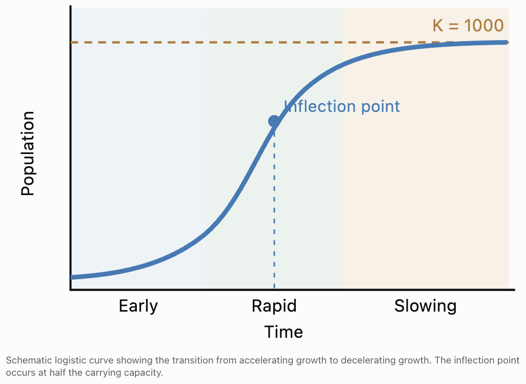
Region 1: Early growth
When the population is small compared with K, resource limitations are relatively weak.
The population increases and its absolute growth rate accelerates.
Region 2: Rapid growth
The population grows quickly.
However, as resource competition increases, the growth rate eventually reaches its maximum and then begins to decline.
Region 3: Slowing growth
As the population approaches carrying capacity, the growth rate decreases toward zero.
The graph becomes nearly horizontal.
The Inflection Point
The inflection point is where the logistic graph changes from curving upward to curving downward.
For the standard logistic growth model with r > 0:
This is also the population at which the instantaneous absolute growth rate is greatest.
For a carrying capacity of 1,000:
The maximum growth rate occurs when the population reaches 500.
Why does maximum growth occur at half the carrying capacity?
At low population sizes, there are relatively few organisms reproducing.
At high population sizes, resource limitations strongly reduce growth.
At half the carrying capacity, the balance between population size and resource availability produces the maximum net growth rate in the standard model.
The maximum instantaneous growth rate is:
Worked Example 3: Maximum Growth Rate
A population has:
K = 2,000
r = 0.3 per year
Calculate the population at maximum growth and the maximum instantaneous growth rate.
Step 1: Find the population at the inflection point.
Step 2: Calculate the maximum growth rate.
The population grows most rapidly when it reaches 1,000 organisms, at an instantaneous rate of 150 organisms per year.
Finding the Time at Which a Population Reaches a Target
Logistic equations can be rearranged using natural logarithms.
Starting with:
Multiply both sides by the denominator:
Divide by P:
Subtract 1:
Divide by A:
Take natural logarithms:
Therefore:
For a population starting below K, this formula applies to target populations between 0 and K.
Worked Example 4: Time to Reach Half the Carrying Capacity
Return to the deer population model:
Find when the population reaches 500 deer.
Step 1: Substitute P(t) = 500.
Step 2: Rearrange.
Step 3: Take natural logarithms.
Since ln(1/9) = −ln(9):
Step 4: Solve.
The deer population reaches 500 after approximately 5.49 years.
At this point, its instantaneous growth rate is greatest.
Worked Example 5: Time to Reach 90% of Carrying Capacity
Using the same model, find when the population reaches 900 deer.
Rearrange:
Take natural logarithms:
The population reaches 90% of carrying capacity after approximately 10.99 years.
Notice that it takes considerably longer to approach the final limiting population than to pass through the middle portion of the curve.
Estimating a Logistic Model from Data
Sometimes the carrying capacity and initial population are known, but the growth parameter r must be estimated.
Suppose a fish population is modelled by:
Given:
-
Carrying capacity K = 5,000 fish.
-
Initial population P₀ = 500 fish.
-
Population after 4 years P(4) = 1,500 fish.
Find r.
Step 1: Calculate A
Step 2: Substitute the known population
Rearrange:
Step 3: Take natural logarithms
Step 4: Write the model
This model can now be used to estimate the fish population at other times.
In practice, fitting a logistic curve to several observations is generally preferable to estimating the growth parameter from only two population measurements.
Logistic Growth in Real-World Populations
Wildlife Populations
Logistic models can describe how populations of rabbits, deer, or other animals increase in environments with limited food and space. Carrying capacity represents the population level supported under the assumed environmental conditions.
Bacterial Growth
Bacterial populations may initially grow rapidly but slow as nutrients become depleted and waste accumulates. Logistic growth can approximate this pattern in some circumstances.
Fisheries Management
Population models can help researchers investigate fish population growth and evaluate sustainable harvesting strategies. Real fisheries often require more detailed models incorporating age structure, environmental changes, and harvesting.
Forest Regeneration
Logistic-type models can describe some aspects of vegetation establishment, coverage, or population growth as space and resources become limiting.
Authentic Application: Managing a Wildlife Reserve
A wildlife reserve has a carrying capacity of approximately 2,500 deer.
The current population is 250 deer, and the intrinsic growth parameter is 0.25 per year.
The reserve wants to estimate the population after 10 years and determine when it will reach 2,000 deer.
Part A: Develop the model
K = 2500
P₀ = 250
r = 0.25
Calculate A:
Therefore:
Part B: Predict the population after 10 years
Since e⁻²·⁵ ≈ 0.082085:
The predicted population after 10 years is approximately 1,438 deer.
Part C: Find when the population reaches 2,000
Rearrange:
Take natural logarithms:
The population is predicted to reach 2,000 deer after approximately 14.33 years.
Part D: Evaluate the model
The model assumes that:
-
Carrying capacity remains at 2,500 deer.
-
The intrinsic growth parameter remains constant.
-
The population responds smoothly to density-dependent limitations.
-
There are no major changes in habitat, disease, hunting, or food supply.
A real wildlife reserve should monitor the population and update its model as new information becomes available.
The model supports planning but should not be treated as an exact prediction.
Limitations of Logistic Growth Models
Although logistic growth is more realistic than unlimited exponential growth in many situations, it is still a simplified mathematical model.
Constant carrying capacity
The standard model assumes that K remains constant.
In reality, environmental conditions can change.
Constant intrinsic growth parameter
The parameter r is assumed to remain constant.
Birth rates, death rates, and environmental conditions may vary over time.
Immediate response to population density
The basic model assumes that population growth responds immediately to population size.
Real populations may experience time delays, seasonal reproduction, or other complex effects.
No age or spatial structure
The model treats the population as a single quantity.
Real populations may contain different age groups, reproductive stages, and geographical subpopulations.
Population fluctuations
Real populations may oscillate around carrying capacity or experience sudden declines.
The standard continuous logistic model with constant parameters does not produce sustained oscillations.
Not all S-shaped patterns are logistic
An S-shaped graph does not automatically prove that a logistic model is appropriate.
Other mathematical models can produce similar curves.
Researchers should evaluate the fit, residuals, assumptions, and biological plausibility before selecting a model.
Common Mistakes
Mistake 1: Assuming logistic growth continues indefinitely
Logistic growth approaches a limiting value.
Correction: Identify the carrying capacity and explain the long-term behaviour.
Mistake 2: Confusing carrying capacity with initial population
K represents the long-term limiting population, while P₀ represents the population at time zero.
Correction: Interpret each parameter separately.
Mistake 3: Assuming growth is fastest at carrying capacity
At carrying capacity, the standard logistic model predicts zero net growth.
Correction: Maximum instantaneous growth occurs at P = K/2.
Mistake 4: Assuming logistic growth is always increasing
If the initial population is above carrying capacity, the standard model predicts a decrease toward K.
Correction: Compare the initial population with K before describing the graph.
Mistake 5: Using exponential growth when resources are limited
Exponential growth may become unrealistic over long periods.
Correction: Consider whether a logistic or another resource-limited model is more appropriate.
Mistake 6: Confusing r with the actual population growth rate
The parameter r is the intrinsic per-capita growth parameter.
The actual instantaneous relative growth rate is:
r(1 − P/K).
Correction: Account for population density when interpreting growth.
Mistake 7: Assuming carrying capacity is permanent
Environmental changes can alter the resources available to a population.
Correction: Treat K as a model parameter dependent on environmental conditions.
Key Terms
-
Logistic Growth: Population growth that slows as the population approaches carrying capacity.
-
Exponential Growth: Growth at a constant proportional rate without an explicit carrying-capacity limit.
-
Carrying Capacity (K): The population size supported by an environment under the conditions assumed by the model.
-
Intrinsic Growth Parameter (r): A parameter describing the potential per-capita growth rate at low population density.
-
Initial Population (P₀): The population present at time zero.
-
Sigmoid Curve: An S-shaped curve.
-
Inflection Point: The point where a curve changes concavity.
-
Density-Dependent Limitation: A factor whose effect on population growth changes with population density.
-
Population Growth Rate: The rate at which population size changes over time.
-
Equilibrium Population: A population size at which the model predicts zero net change.
-
Horizontal Asymptote: A horizontal line approached by a graph as the independent variable increases or decreases without bound.
-
Limiting Factor: An environmental factor restricting population growth.
-
Mathematical Model: A mathematical representation of a real-world system.
-
Model Parameter: A numerical quantity that controls the behaviour of a model.
-
Population Dynamics: The study of how populations change over time.
-
Environmental Resistance: The combined effects of environmental factors that limit population growth.
Key Takeaways
-
Logistic growth describes population growth under limited resources.
-
Logistic growth often produces an S-shaped curve.
-
Exponential growth assumes a constant relative growth rate and does not include carrying capacity.
-
Carrying capacity is the limiting population size in the standard logistic model.
-
The logistic function is P(t) = K/(1 + Ae⁻ʳᵗ).
-
The constant A is determined by the initial population.
-
Growth is initially approximately exponential when the population is much smaller than K.
-
The instantaneous growth rate is greatest when P = K/2.
-
As the population approaches K, the growth rate approaches zero.
-
Natural logarithms can be used to determine when a population reaches a specified size.
-
Logistic models are useful in ecology, wildlife management, microbiology, and population studies.
-
Real-world models must be evaluated for assumptions, limitations, and changing environmental conditions.
Check Your Understanding
Questions
Question 1: Understanding Logistic Growth
Explain why a population may initially grow exponentially but later follow a logistic growth pattern.
Question 2: Comparing Growth Models
State two differences between exponential and logistic growth.
Question 3: Carrying Capacity
A lake can sustain approximately 8,000 fish.
Explain what this means in terms of carrying capacity.
Question 4: Identifying Parameters
Consider:
P(t) = 1500/(1 + 14e⁻⁰·³ᵗ)
Identify K, A, and r.
Question 5: Initial Population
For the model in Question 4, calculate P(0).
Question 6: Predicting Population Size
A population follows:
P(t) = 2000/(1 + 9e⁻⁰·⁴ᵗ)
Calculate the population after 5 years.
Question 7: Maximum Growth
A logistic population has carrying capacity K = 4,000 and intrinsic growth parameter r = 0.2 per year.
Find the population at maximum growth and the maximum instantaneous growth rate.
Question 8: Developing a Model
A population begins with 200 organisms in an environment with carrying capacity 1,000.
The intrinsic growth parameter is 0.3 per year.
Develop a logistic population model.
Question 9: Solving for Time
A population follows:
P(t) = 1000/(1 + 9e⁻⁰·⁵ᵗ)
Find when the population reaches 500.
Question 10: Long-Term Behaviour
Determine the long-term population predicted by:
P(t) = 6000/(1 + 5e⁻⁰·²ᵗ).
Question 11: Interpreting a Graph
A logistic curve rises steeply and then becomes almost horizontal.
Explain what is happening to the population and its growth rate.
Question 12: Real-World Modelling
A wildlife population grows rapidly for several years before its growth slows.
Explain how carrying capacity and resource competition could account for this pattern.
Question 13: Model Evaluation
Identify two assumptions of the standard logistic growth model and explain how they might be violated in a real ecosystem.
Question 14: Challenging Application
A population initially contains 500 organisms. Its carrying capacity is 5,000, and its intrinsic growth parameter is 0.25 per year.
a) Develop a logistic growth model.
b) Calculate the population after 8 years.
c) Find when the population reaches 2,500.
Fully Worked Answers
Answer 1: Understanding Logistic Growth
A population may initially grow approximately exponentially because resources are abundant and competition is limited.
As the population increases, food, water, space, and other resources become more limited.
These density-dependent factors reduce the population's relative growth rate.
Eventually, the population approaches carrying capacity, producing a logistic growth pattern.
Answer 2: Comparing Growth Models
Difference 1: Exponential growth does not include a carrying-capacity limit, while logistic growth does.
Difference 2: Exponential growth has a constant relative growth rate, while logistic growth has a relative growth rate that decreases as population size approaches carrying capacity.
Exponential growth produces a J-shaped curve, while logistic growth beginning well below K typically produces an S-shaped curve.
Answer 3: Carrying Capacity
The carrying capacity is approximately 8,000 fish.
This means the lake is estimated to support a long-term population of around 8,000 fish under the assumed environmental conditions.
If the population is below carrying capacity, it may increase.
If it exceeds carrying capacity, the standard logistic model predicts a decrease toward 8,000.
Answer 4: Identifying Parameters
Given:
Compare with:
Therefore:
-
K = 1500
-
A = 14
-
r = 0.3 per time unit
Answer 5: Initial Population
At t = 0:
The initial population is 100 organisms.
Answer 6: Predicting Population Size
Given:
Substitute t = 5:
Since e⁻² ≈ 0.135335:
The predicted population after five years is approximately 902 organisms.
Answer 7: Maximum Growth
Given:
K = 4000
r = 0.2
The population at maximum growth is:
The maximum instantaneous growth rate is:
Answer 8: Developing a Model
Given:
P₀ = 200
K = 1000
r = 0.3
Calculate A:
Therefore:
Answer 9: Solving for Time
Given:
Set P(t) = 500.
Rearrange:
Take natural logarithms:
The population reaches 500 after approximately 4.39 time units.
Answer 10: Long-Term Behaviour
Given:
As t approaches infinity:
Therefore:
The carrying capacity is 6,000.
Answer 11: Interpreting a Graph
The steep part of the curve indicates rapid population growth.
As the curve becomes nearly horizontal, the population approaches carrying capacity.
The instantaneous growth rate decreases toward zero because density-dependent limitations become increasingly important.
The population continues increasing, but more slowly.
Answer 12: Real-World Modelling
When the wildlife population is small, resources are abundant and competition is relatively weak.
As the population grows, more animals compete for food, water, shelter, and space.
These limitations reduce the relative growth rate.
Eventually, the population approaches the carrying capacity of the environment, and net population growth becomes small.
This produces the characteristic logistic growth pattern.
Answer 13: Model Evaluation
Assumption 1: Constant carrying capacity
The model assumes that K remains constant.
A drought, habitat destruction, or seasonal change could reduce available resources and alter carrying capacity.
Assumption 2: Constant intrinsic growth parameter
The model assumes that r remains constant.
Disease outbreaks, changes in reproduction, or environmental disturbances could change the population's growth potential.
These limitations mean that real population models should be monitored and updated.
Answer 14: Challenging Application
Given:
P₀ = 500
K = 5000
r = 0.25
Part a: Develop the model.
Calculate A:
Therefore:
Part b: Calculate the population after 8 years.
The predicted population after eight years is approximately 2,254 organisms.
Part c: Find when the population reaches 2,500.
Rearrange:
Take natural logarithms:
The population reaches half its carrying capacity after approximately 8.79 years.
At that point, the instantaneous growth rate is greatest.
Final Reflection
Logistic growth models provide a more realistic description of many populations than unrestricted exponential growth because they account for environmental limitations.
Their characteristic S-shaped curves reveal how population growth changes over time: initially accelerating, then reaching a maximum rate, and finally slowing as carrying capacity is approached.
The logistic function:
connects exponential functions, natural logarithms, calculus, and real-world population dynamics.
The central idea is that population growth depends not only on the number of organisms present, but also on the resources available to support them.
Understanding logistic growth helps us interpret ecological systems, evaluate population forecasts, and make more informed decisions about managing limited resources.
5. Comparing Mathematical Models
Learning outcomes
- I can compare linear, quadratic, exponential, logarithmic, and logistic models.
- I can identify the most appropriate model for a situation.
- I can justify model selection.
- I can interpret mathematical models critically.
- I can evaluate model limitations.
Introduction
Mathematics allows us to describe, explain, and predict patterns in the world around us. However, different situations require different mathematical models.
Consider five situations:
-
A taxi company charges a fixed booking fee plus a constant amount per kilometre.
-
A ball is thrown upward, rises to a maximum height, and then falls.
-
A bacterial population grows rapidly when resources are abundant.
-
The time needed to complete a task decreases as experience increases, but improvements gradually become smaller.
-
A wildlife population grows quickly before slowing as it approaches the environmental carrying capacity.
Although all five situations involve relationships between variables, they do not follow the same mathematical pattern.
A mathematical model is a mathematical representation of a real-world situation. Models may use equations, functions, graphs, tables, or statistical relationships to describe how quantities are connected.
Choosing an appropriate model is one of the most important parts of mathematical problem-solving. A model must not only fit the available data but also make sense in the context of the situation.
In this lesson, we will compare five important types of models: linear, quadratic, exponential, logarithmic, and logistic. We will learn how to recognise their patterns, select appropriate models, justify our choices, interpret predictions, and evaluate the limitations of mathematical modelling.
What Is a Mathematical Model?
A mathematical model uses mathematical relationships to represent important features of a real system.
For example, suppose a delivery company charges $8 plus $3 for every kilometre travelled.
The total cost can be modelled by:
C(d) = 8 + 3d
where:
-
C = total delivery cost in dollars.
-
d = distance travelled in kilometres.
-
8 = fixed charge.
-
3 = charge per kilometre.
The model allows us to calculate costs for different distances.
For a delivery of 12 km:
C(12) = 8 + 3(12)
C(12) = 8 + 36
C(12) = $44
However, the model assumes that the pricing rules remain unchanged. It may not apply if the company introduces discounts, maximum charges, or additional fees.
This illustrates an essential principle:
A mathematical model is a simplified representation of reality, not reality itself.
The Five Major Mathematical Models
The following models describe different patterns of change.
|
Model |
General form |
Characteristic behaviour |
|---|---|---|
|
Linear |
y = mx + b |
Constant rate of change |
|
Quadratic |
y = ax² + bx + c |
Parabolic relationship |
|
Exponential |
y = Abˣ or Aeᵏˣ |
Constant multiplicative change |
|
Logarithmic |
y = a ln(x) + b |
Rapid initial change followed by slowing change |
|
Logistic |
y = K/(1 + Ae⁻ʳˣ) |
Growth that approaches a limiting value |
Each model has distinctive graphical features and mathematical properties.
Visual Comparison of the Models
Explore five mathematical model shapes
Select a model to see its characteristic graph and equation. These are illustrative examples rather than fitted real-world datasets.
y = 2x + 1
A straight line with a constant slope.
Linear Models
A linear model describes a relationship with a constant rate of change.
The general equation is:
y = mx + b
where:
-
m = slope or rate of change.
-
b = y-intercept or initial value.
Characteristics
-
Graph is a straight line.
-
Equal changes in x produce equal changes in y.
-
Slope is constant.
-
The model may increase, decrease, or remain constant.
Worked Example 1: Taxi Fare
A taxi company charges a base fare of $5 and $2.50 per kilometre.
The model is:
C(d) = 5 + 2.5d
Calculate the fare for a 14 km journey.
C(14) = 5 + 2.5(14)
C(14) = 5 + 35
C(14) = $40
Interpreting the model
The slope, 2.5, represents the additional cost per kilometre.
The intercept, 5, represents the fixed starting charge.
A linear model is appropriate because the cost increases by a constant amount for every additional kilometre.
When is a linear model appropriate?
Linear models are useful when the relationship has a reasonably constant additive rate of change.
Examples include fixed-rate wages, simple pricing systems, uniform motion, and some short-term trends.
However, linear models may become unrealistic if rates change, limits are reached, or the underlying relationship is nonlinear.
Quadratic Models
A quadratic model describes a relationship involving a squared variable.
The general equation is:
y = ax² + bx + c, where a ≠ 0.
Its graph is a parabola.
Characteristics
-
Graph is U-shaped or inverted U-shaped.
-
May have a maximum or minimum.
-
Rate of change is not constant.
-
Second differences are constant for equally spaced x-values.
-
Often describes relationships involving acceleration, area, or optimisation.
Worked Example 2: Projectile Motion
A ball is thrown upward from a height of 2 metres.
Its height is modelled by:
h(t) = −5t² + 20t + 2
where t is measured in seconds.
Find the maximum height.
For a quadratic function, the vertex occurs at:
t = −b/(2a)
Here:
a = −5
b = 20
Therefore:
t = −20/[2(−5)]
t = 2 seconds
Substitute:
h(2) = −5(2²) + 20(2) + 2
h(2) = −20 + 40 + 2
Maximum height = 22 m
The quadratic model is appropriate because the ball experiences approximately constant downward acceleration.
Why not use a linear model?
A linear model assumes constant vertical velocity.
The ball slows while rising, stops momentarily at its maximum height, and accelerates downward.
Its vertical velocity changes continuously, so a quadratic height–time model is more appropriate when air resistance is neglected.
Exponential Models
Exponential models describe processes with constant proportional change.
Common forms are:
y = Abˣ
and
y = Aeᵏˣ
where A is the initial quantity.
Characteristics
-
Equal increases in x produce equal multiplication factors.
-
The absolute rate of change depends on the current quantity.
-
Growth is unbounded when the growth rate remains positive.
-
Decay approaches zero when the decay constant is negative.
-
Often describes compound interest, early population growth, and first-order decay.
Worked Example 3: Bacterial Growth
A bacterial population begins with 300 organisms and doubles every 4 hours.
The model is:
P(t) = 300 × 2^(t/4)
Calculate the population after 12 hours.
P(12) = 300 × 2^(12/4)
P(12) = 300 × 2³
P(12) = 300 × 8
P(12) = 2,400 bacteria
Why is an exponential model appropriate?
The population multiplies by the same factor over each four-hour interval.
A linear model would assume the same number of bacteria is added every four hours, rather than the population doubling.
Important limitation
Exponential growth is often suitable only while resources remain sufficiently abundant.
Eventually, competition, nutrient depletion, or other environmental constraints may reduce the growth rate.
Logarithmic Models
A logarithmic model describes a relationship that changes rapidly at first but then changes more slowly.
A common form is:
y = a ln(x) + b, where x > 0.
The function ln(x) is the natural logarithm.
Characteristics
-
Domain is restricted to positive x-values in the basic form.
-
When a > 0, the graph increases at a decreasing rate.
-
When a < 0, the graph decreases at a decreasing absolute rate.
-
The basic graph has a vertical asymptote at x = 0.
-
Logarithmic functions are inverses of exponential functions.
Worked Example 4: Learning and Experience
A simplified model for a worker's performance score is:
S(x) = 40 + 12ln(x)
where x represents the number of completed practice sessions, with x ≥ 1.
Calculate the predicted score after 10 sessions.
S(10) = 40 + 12ln(10)
Since ln(10) ≈ 2.3026:
S(10) ≈ 40 + 12(2.3026)
S(10) ≈ 40 + 27.6312
S(10) ≈ 67.63
Interpreting the model
The score increases as the number of sessions increases, but the improvement per additional session becomes smaller.
This illustrates diminishing returns.
However, the logarithmic model does not have a finite upper limit. It would eventually predict arbitrarily large scores if extended indefinitely.
If performance has a strict maximum, another model may be more suitable for long-term predictions.
Logistic Models
A logistic model describes growth that slows as a quantity approaches a limiting value.
A common form is:
P(t) = K/(1 + Ae⁻ʳᵗ)
where:
-
K = carrying capacity or limiting value.
-
A = constant determined by the initial quantity.
-
r = intrinsic growth parameter.
-
t = time.
Characteristics
-
Usually produces an S-shaped graph when starting well below K.
-
Initially resembles exponential growth.
-
Growth slows as the population approaches carrying capacity.
-
Maximum instantaneous growth occurs at P = K/2 in the standard model.
-
The population approaches K as time increases.
Worked Example 5: Wildlife Population
A wildlife population follows:
P(t) = 2000/(1 + 19e⁻⁰·⁴ᵗ)
Calculate the population after 10 years.
P(10) = 2000/(1 + 19e⁻⁴)
Since e⁻⁴ ≈ 0.0183156:
P(10) ≈ 2000/[1 + 19(0.0183156)]
P(10) ≈ 2000/1.347997
P(10) ≈ 1,484 organisms
Interpreting the model
The carrying capacity is 2,000 organisms.
The initial population is:
P(0) = 2000/(1 + 19)
P(0) = 100
The model predicts that the population increases from 100 and gradually approaches 2,000.
A logistic model is appropriate when population growth is limited by environmental resources.
Identifying the Most Appropriate Model
One of the most important modelling skills is recognising which mathematical relationship best describes a situation.
Recognising patterns in data
|
Observed pattern |
Likely model |
|---|---|
|
Constant first differences |
Linear |
|
Constant second differences |
Quadratic |
|
Approximately constant ratios |
Exponential |
|
Rapid initial change that gradually slows without a fixed bound |
Logarithmic |
|
S-shaped growth approaching a stable limit |
Logistic |
These patterns are useful clues, but they are not sufficient by themselves to establish which model is correct.
The underlying context and assumptions must also be considered.
Worked Example 6: Identifying a Model from a Table
Consider the following data.
|
x |
y |
|---|---|
|
1 |
5 |
|
2 |
9 |
|
3 |
13 |
|
4 |
17 |
|
5 |
21 |
Calculate the first differences:
9 − 5 = 4
13 − 9 = 4
17 − 13 = 4
21 − 17 = 4
The first differences are constant.
Therefore, a linear model is appropriate.
The slope is 4.
Using y = mx + b:
5 = 4(1) + b
b = 1
The model is:
y = 4x + 1
Worked Example 7: Identifying Quadratic Growth
Consider:
|
x |
y |
|---|---|
|
0 |
2 |
|
1 |
5 |
|
2 |
10 |
|
3 |
17 |
|
4 |
26 |
First differences:
3, 5, 7, 9
Second differences:
2, 2, 2
The constant second differences suggest a quadratic model.
The equation is:
y = x² + 2x + 2
Check x = 3:
y = 3² + 2(3) + 2
y = 9 + 6 + 2
y = 17
The equation matches the data.
Worked Example 8: Identifying Exponential Growth
Consider:
|
x |
y |
|---|---|
|
0 |
100 |
|
1 |
150 |
|
2 |
225 |
|
3 |
337.5 |
|
4 |
506.25 |
Calculate successive ratios:
150/100 = 1.5
225/150 = 1.5
337.5/225 = 1.5
506.25/337.5 = 1.5
The ratio is constant.
Therefore, an exponential model is appropriate.
y = 100(1.5)ˣ
The quantity increases by 50% for every one-unit increase in x.
Distinguishing Logarithmic and Logistic Patterns
Logarithmic and logistic models can be difficult to distinguish because both may show growth that gradually slows.
However, their long-term behaviour is fundamentally different.
A logarithmic model such as:
y = 10 + 5ln(x)
continues increasing without a finite upper limit, although its rate of increase becomes smaller.
A logistic model such as:
y = 100/(1 + 9e⁻⁰·⁵ˣ)
approaches a fixed upper limit of 100.
Comparing their behaviour
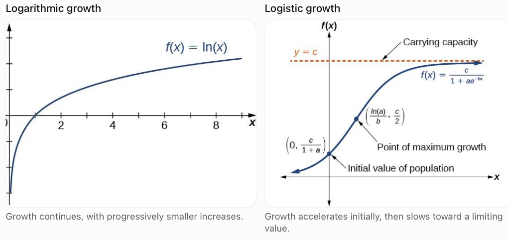
The distinction matters when making long-term predictions.
For example, a learning-performance score that cannot exceed 100 may be better represented by a bounded model than by a logarithmic function that eventually exceeds 100.
A logistic model is one possible bounded model, although it should only be selected when its shape and assumptions are appropriate.
A Systematic Method for Selecting a Model
Choosing a mathematical model should involve more than looking at a graph and selecting the closest-looking curve.
A reliable process follows several stages.
Model selection process
1. Define the problem and variables
2. Examine the data and graph
3. Identify plausible model types
4. Fit models and check assumptions
5. Compare performance and interpretability
6. Validate predictions and communicate limitations
Step 1: Understand the situation
Ask what the variables represent and what is known about their relationship.
For example, does a price increase by a fixed amount, or does a population increase by a fixed percentage?
Step 2: Examine the data
Construct an appropriate scatter plot and investigate patterns.
Look for straight-line trends, curvature, changing growth rates, or evidence of a limiting value.
Step 3: Identify candidate models
Consider which models are mathematically and scientifically plausible.
Do not assume that the most complicated model is necessarily the best.
Step 4: Fit the models
Estimate the parameters using the available data.
For example, linear regression can estimate a slope and intercept, while nonlinear regression can estimate logistic model parameters.
Step 5: Evaluate model performance
Compare prediction errors and examine residuals.
Step 6: Interpret and validate
Determine whether the selected model makes sense in context and performs adequately on data not used to fit it.
Justifying Model Selection
A strong model justification should contain four elements:
Observed pattern + Mathematical evidence + Contextual reasoning + Limitations
Example: Choosing a Model for Population Growth
Suppose a researcher measures a population over 12 years.
The population grows rapidly at first but begins to level off near 5,000 organisms.
A justified explanation might be:
"A logistic model is appropriate because the population initially increases rapidly, but its growth rate decreases as the population approaches approximately 5,000 organisms. This suggests a carrying-capacity limitation. An exponential model would predict unlimited growth and is therefore less plausible over the long term. However, the logistic model assumes that carrying capacity and the intrinsic growth parameter remain constant."
This explanation is stronger than simply saying:
"The graph looks like an S, so the model is logistic."
The first explanation connects the mathematical pattern to the underlying situation.
Evaluating Model Performance
Different models can be fitted to the same dataset.
The model that produces the smallest error on the training data is not necessarily the most appropriate model.
A good model should also make reliable predictions and have assumptions consistent with the situation.
Residuals
A residual is the difference between an observed value and its predicted value.
Residual = Observed value − Predicted value
In symbols:
eᵢ = yᵢ − ŷᵢ
Where:
-
yᵢ = observed value.
-
ŷᵢ = predicted value.
-
eᵢ = residual.
A positive residual means the model underestimated the observation.
A negative residual means the model overestimated the observation.
Worked Example 9: Calculating Residuals
Suppose a model predicts examination scores.
|
Student |
Actual score |
Predicted score |
Residual |
|---|---|---|---|
|
A |
70 |
68 |
2 |
|
B |
75 |
78 |
−3 |
|
C |
82 |
80 |
2 |
|
D |
88 |
85 |
3 |
|
E |
90 |
94 |
−4 |
For Student A:
Residual = 70 − 68 = 2
For Student B:
Residual = 75 − 78 = −3
Residuals help identify patterns the model has failed to explain.
Interpreting residual plots
A suitable model often produces residuals scattered around zero without a systematic pattern.
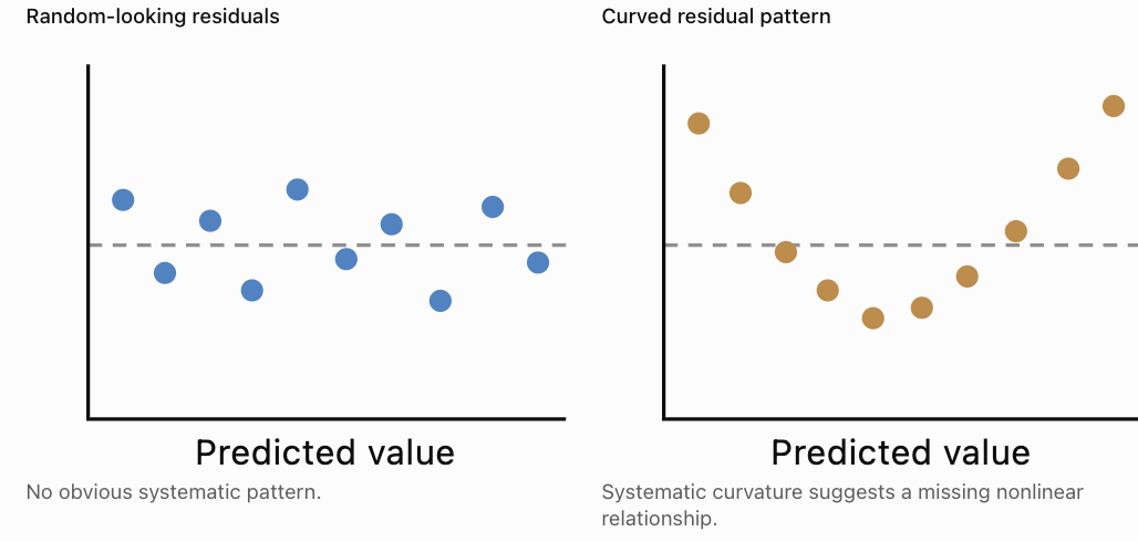
A curved residual pattern from a linear model may suggest that a quadratic or another nonlinear model would be more appropriate.
However, random-looking residuals alone do not prove that a model is valid.
Measuring Model Accuracy
Several numerical measures help compare model performance.
Mean Absolute Error (MAE)
MAE is the average absolute prediction error.
Mean Squared Error (MSE)
MSE is the average squared prediction error.
Root Mean Squared Error (RMSE)
RMSE is the square root of MSE.
MAE and RMSE are measured in the same units as the response variable.
RMSE penalises larger errors more heavily than MAE.
Coefficient of determination (R²)
R² measures the proportion of variation in the response explained by a model relative to a mean-only baseline, using the usual squared-error definition.
For ordinary least-squares models with an intercept, it typically lies between 0 and 1 on the training data.
However, R² can be negative for some models or when evaluated on new data.
A high R² does not automatically mean a model is appropriate.
A model can fit observed data well while making poor predictions outside the observed range.
Worked Example 10: Comparing Two Models
Suppose a researcher fits a linear model and a quadratic model to the same dataset.
The models produce the following residuals on an independent validation dataset.
|
Observation |
Linear residual |
Quadratic residual |
|---|---|---|
|
1 |
4 |
2 |
|
2 |
−3 |
−2 |
|
3 |
5 |
1 |
|
4 |
−4 |
−2 |
|
5 |
2 |
1 |
Calculate RMSE for each model.
Linear model
Square the residuals:
4² = 16
(−3)² = 9
5² = 25
(−4)² = 16
2² = 4
Sum:
16 + 9 + 25 + 16 + 4 = 70
MSE = 70/5 = 14
RMSE = √14
RMSE ≈ 3.74
Quadratic model
Square the residuals:
2² = 4
(−2)² = 4
1² = 1
(−2)² = 4
1² = 1
Sum:
4 + 4 + 1 + 4 + 1 = 14
MSE = 14/5 = 2.8
RMSE = √2.8
RMSE ≈ 1.67
Interpretation
The quadratic model has a lower validation RMSE.
It therefore makes more accurate predictions on this validation dataset according to RMSE.
This supports selecting the quadratic model, provided its assumptions and contextual interpretation are also reasonable.
We should still investigate whether the improvement is consistent across other data and whether the model generalises beyond the observed range.
Overfitting and Underfitting
Two important problems can occur when selecting models.
Underfitting
Underfitting occurs when a model is too simple to capture important patterns.
For example, a straight line may fit poorly when the underlying relationship is strongly curved.
Overfitting
Overfitting occurs when a model captures random variation or noise in the training data rather than the underlying relationship.
For example, a high-degree polynomial might pass through every observed point but behave unpredictably between or beyond those points.
Balancing complexity and accuracy
The goal is not to find the most complicated model.
It is to find a model that captures the important relationship while making reliable predictions.
This is why model validation matters.
A common approach is to fit models using training data and compare their performance using separate validation data.
Interpolation and Extrapolation
Mathematical models are often used to estimate values that were not directly observed.
Interpolation
Interpolation means predicting within the range of the observed data.
For example, if a model was developed using temperatures between 10°C and 30°C, estimating a value at 20°C is interpolation.
Extrapolation
Extrapolation means predicting outside the observed range.
Estimating a value at 60°C using the same model would be extrapolation.
Extrapolation is generally more uncertain because the relationship may change outside the observed conditions.
Example: Population Predictions
Suppose a population has been observed for five years and has increased from 100 to 300.
An exponential model may fit these early observations well.
However, predicting the population 100 years into the future could be unrealistic if food and space are limited.
A logistic model might be more plausible, but estimating its carrying capacity from only the early growth phase can also be highly uncertain.
A model's reliability depends on both its mathematical fit and the conditions under which it is used.
Real-World Applications of Model Selection
Transport and Pricing — Linear
A fixed starting charge plus a constant charge per kilometre is naturally modelled by a linear function. Real pricing may also include time charges and surcharges.
Projectile Motion — Quadratic
Height as a function of time is quadratic when vertical acceleration is constant and air resistance can be neglected.
Early Microbial Growth — Exponential
Populations may grow approximately exponentially when resources are plentiful and the relative growth rate is nearly constant.
Learning and Practice — Logarithmic
Some measures of improvement show rapid early gains followed by diminishing returns. A logarithmic model may describe part of this pattern, although a bounded model may be more suitable over longer periods.
Population Ecology — Logistic
Logistic models can represent population growth that slows as resources become limiting and the population approaches carrying capacity.
Authentic Modelling Investigation: Selecting the Best Population Model
A wildlife researcher records the population of an introduced species over several years.
The following hypothetical data are collected.
|
Year |
Population |
|---|---|
|
0 |
100 |
|
2 |
182 |
|
4 |
303 |
|
6 |
451 |
|
8 |
599 |
|
10 |
721 |
|
12 |
806 |
The researcher wants to select a model for future population predictions.
Step 1: Examine the pattern
The population increases throughout the observation period.
However, the increases over successive two-year intervals are:
82, 121, 148, 148, 122, 85
The increases initially become larger and then smaller.
This suggests that the population's absolute growth rate is beginning to slow.
Step 2: Consider possible models
A linear model would assume a constant increase per year.
An exponential model would assume a constant proportional growth rate.
A logistic model allows growth to accelerate initially and then slow as carrying capacity is approached.
The logistic model is a plausible candidate.
Step 3: Propose a logistic model
Suppose the researcher estimates a carrying capacity of 900 organisms.
A candidate model is:
P(t) = 900/(1 + 8e⁻⁰·³ᵗ)
The initial population is:
P(0) = 900/(1 + 8)
P(0) = 100
The model reproduces the initial observation.
Step 4: Compare predictions with observations
|
Year |
Observed |
Logistic prediction (approx.) |
|---|---|---|
|
0 |
100 |
100 |
|
2 |
182 |
167 |
|
4 |
303 |
264 |
|
6 |
451 |
388 |
|
8 |
599 |
521 |
|
10 |
721 |
644 |
|
12 |
806 |
739 |
The model captures the general S-shaped pattern but systematically underestimates the later observations.
This suggests that the proposed parameters require adjustment.
It would be inappropriate to claim that the logistic model is accurate simply because its graph has the expected shape.
Step 5: Improve the investigation
The researcher could:
-
Fit the logistic parameters using nonlinear regression rather than choosing them manually.
-
Compare the fitted logistic model with exponential and other plausible models.
-
Examine residuals for systematic patterns.
-
Evaluate predictions using later observations.
-
Investigate whether the estimated carrying capacity is biologically realistic.
Step 6: Communicate a justified conclusion
"The observed population initially experienced increasing absolute growth, followed by smaller increases in later years. This pattern is consistent with a logistic-type growth process. However, the proposed logistic equation systematically underestimated the observations, so its parameters should be re-estimated and its predictions validated before it is used for management decisions."
This is an example of critical mathematical modelling: the researcher considers both the observed pattern and the quality of the fitted equation.
Common Mistakes
Mistake 1: Selecting a model based only on its appearance
Different models can produce similar curves over short intervals.
Correction: Examine mathematical patterns, assumptions, and residuals.
Mistake 2: Assuming the model with the highest R² is always best
A complicated model may fit training data well but predict poorly.
Correction: Consider validation performance, model complexity, and contextual plausibility.
Mistake 3: Confusing linear and exponential growth
Linear growth involves constant additions. Exponential growth involves constant multiplication factors.
Correction: Compare differences and ratios.
Mistake 4: Confusing logarithmic and logistic growth
A logarithmic function continues increasing without a finite upper bound, while a standard increasing logistic function approaches carrying capacity.
Correction: Examine long-term behaviour.
Mistake 5: Ignoring the domain
Some models are mathematically defined for values that make no sense in the situation.
Correction: State meaningful restrictions on the independent variable.
Mistake 6: Treating model predictions as exact
Predictions are estimates that depend on assumptions and data quality.
Correction: Communicate uncertainty and limitations.
Mistake 7: Extrapolating too far
A model may work within the observed range but fail outside it.
Correction: Be cautious when making long-term predictions.
Mistake 8: Ignoring the meaning of parameters
A mathematical equation is more useful when its coefficients can be interpreted in context.
Correction: Explain slopes, initial values, growth rates, turning points, and carrying capacities.
Key Terms
-
Mathematical Model: A mathematical representation of a real-world relationship or system.
-
Linear Model: A model with a constant additive rate of change.
-
Quadratic Model: A model containing a squared variable, producing a parabolic graph.
-
Exponential Model: A model with a constant proportional rate of change.
-
Logarithmic Model: A model involving a logarithmic relationship.
-
Logistic Model: A model describing growth that approaches a limiting value.
-
Carrying Capacity: The limiting population size in a standard logistic growth model.
-
Slope: The rate of change of a linear function.
-
Vertex: The maximum or minimum point of a parabola.
-
Growth Rate: A measure of how quickly a quantity increases.
-
Residual: The difference between an observed value and a predicted value.
-
Mean Absolute Error: The average absolute prediction error.
-
Root Mean Squared Error: The square root of the average squared prediction error.
-
Coefficient of Determination (R²): A measure comparing a model's squared prediction errors with those of a mean-only baseline.
-
Underfitting: Failure to capture important patterns because a model is too simple.
-
Overfitting: Fitting random variation rather than the underlying relationship.
-
Interpolation: Prediction within the observed data range.
-
Extrapolation: Prediction outside the observed data range.
-
Model Validation: Evaluating how well a model performs on data not used to fit it.
-
Model Assumption: A condition under which a mathematical model is intended to apply.
-
Model Limitation: A restriction on the accuracy, usefulness, or applicability of a model.
Key Takeaways
-
Linear models describe constant additive change.
-
Quadratic models describe parabolic relationships and can contain maxima or minima.
-
Exponential models describe constant proportional change.
-
Logarithmic models can describe rapidly changing relationships that gradually slow.
-
Logistic models describe growth that approaches a carrying capacity.
-
Differences, second differences, ratios, and graphical patterns help identify candidate models.
-
Model selection should consider mathematical fit and real-world context.
-
Residuals and error measures help evaluate model performance.
-
A more complicated model is not automatically a better model.
-
Predictions outside the observed range require particular caution.
-
Every mathematical model depends on assumptions.
-
A justified model selection explains why the model is appropriate and acknowledges its limitations.
Check Your Understanding
Questions
Question 1: Identifying Models
Identify the most appropriate model type for each situation.
a) A company charges $15 plus $4 per item delivered.
b) A ball is thrown vertically upward.
c) A population doubles every three years.
d) A quantity increases rapidly at first, then more slowly, without an assumed finite limit.
e) A population grows toward an environmental carrying capacity.
Question 2: Linear Modelling
A company charges a fixed fee of $12 plus $3 per kilometre.
Write a model and calculate the cost for 15 km.
Question 3: Quadratic Modelling
A projectile's height is:
h(t) = −5t² + 30t + 2
Find the time at which the projectile reaches its maximum height and calculate that height.
Question 4: Exponential Modelling
A population begins with 200 organisms and increases by 25% each year.
Write a model and calculate the population after four years.
Question 5: Logarithmic Modelling
A simplified performance model is:
S(x) = 30 + 10ln(x)
Calculate S(5), correct to two decimal places.
Question 6: Logistic Modelling
A population follows:
P(t) = 3000/(1 + 14e⁻⁰·²ᵗ)
Determine the carrying capacity and initial population.
Question 7: First Differences
Determine the most appropriate model for:
|
x |
y |
|---|---|
|
1 |
7 |
|
2 |
12 |
|
3 |
17 |
|
4 |
22 |
Question 8: Second Differences
Determine the most appropriate model for:
|
x |
y |
|---|---|
|
0 |
3 |
|
1 |
6 |
|
2 |
11 |
|
3 |
18 |
|
4 |
27 |
Question 9: Exponential Ratios
Determine the most appropriate model for:
|
x |
y |
|---|---|
|
0 |
50 |
|
1 |
100 |
|
2 |
200 |
|
3 |
400 |
Write its equation.
Question 10: Model Accuracy
Two models have validation RMSE values of 4.2 and 2.8.
Which model performs better according to RMSE, and what additional factors should be considered?
Question 11: Residuals
A model predicts 75, but the observed value is 82.
Calculate the residual and interpret it.
Question 12: Extrapolation
A model is developed using data collected over five years.
Explain why predicting 50 years into the future may be unreliable.
Question 13: Model Selection
A population increases rapidly at first, but observations suggest that it is approaching approximately 10,000 organisms.
Explain why a logistic model may be more appropriate than an exponential model.
Question 14: Critical Interpretation
A researcher fits a high-degree polynomial that passes through every observed data point.
Explain why this does not guarantee that the model will make accurate future predictions.
Question 15: Integrated Application
A business records the following sales:
|
Month |
Sales |
|---|---|
|
1 |
120 |
|
2 |
180 |
|
3 |
270 |
|
4 |
405 |
a) Identify a suitable model.
b) Determine the equation.
c) Predict sales in month 5.
d) Explain one limitation of the model.
Fully Worked Answers
Answer 1: Identifying Models
a) Linear — constant additional charge per item.
b) Quadratic — vertical height under approximately constant gravitational acceleration.
c) Exponential — constant doubling factor.
d) Logarithmic — rapid initial increase followed by slower growth without a fixed upper bound.
e) Logistic — growth limited by carrying capacity.
Answer 2: Linear Modelling
The fixed fee is $12, and the charge per kilometre is $3.
C(d) = 12 + 3d
For d = 15:
C(15) = 12 + 3(15)
C(15) = 12 + 45
C(15) = $57
Answer 3: Quadratic Modelling
Given:
h(t) = −5t² + 30t + 2
The maximum occurs at:
t = −b/(2a)
t = −30/[2(−5)]
t = 3 seconds
Substitute:
h(3) = −5(3²) + 30(3) + 2
h(3) = −45 + 90 + 2
Maximum height = 47 m
Answer 4: Exponential Modelling
Initial population = 200.
Growth factor = 1.25.
Model:
P(t) = 200(1.25)ᵗ
After four years:
P(4) = 200(1.25)⁴
P(4) = 200(2.44140625)
P(4) ≈ 488 organisms
Answer 5: Logarithmic Modelling
S(x) = 30 + 10ln(x)
Substitute x = 5:
S(5) = 30 + 10ln(5)
S(5) ≈ 30 + 10(1.609438)
S(5) ≈ 46.09438
S(5) ≈ 46.09
Answer 6: Logistic Modelling
Given:
P(t) = 3000/(1 + 14e⁻⁰·²ᵗ)
The carrying capacity is the numerator:
K = 3000
At t = 0:
P(0) = 3000/(1 + 14)
P(0) = 3000/15
P₀ = 200
Answer 7: First Differences
First differences:
12 − 7 = 5
17 − 12 = 5
22 − 17 = 5
The first differences are constant, so the model is linear.
Slope = 5.
Using y = 5x + b and the point (1, 7):
7 = 5 + b
b = 2
y = 5x + 2
Answer 8: Second Differences
First differences:
3, 5, 7, 9
Second differences:
2, 2, 2
The second differences are constant, so a quadratic model is appropriate.
The equation is:
y = x² + 2x + 3
Check x = 3:
y = 9 + 6 + 3 = 18
The model matches the table.
Answer 9: Exponential Ratios
Successive ratios are:
100/50 = 2
200/100 = 2
400/200 = 2
The constant ratio indicates exponential growth.
Initial value = 50.
Growth factor = 2.
y = 50(2)ˣ
Answer 10: Model Accuracy
The model with RMSE = 2.8 performs better according to validation RMSE because it has a smaller typical squared-error-based prediction magnitude.
However, we should also consider model complexity, residual patterns, assumptions, interpretability, and performance on other representative data.
Answer 11: Residuals
Residual = Observed − Predicted
Residual = 82 − 75
Residual = +7
The positive residual indicates that the model underestimated the observation by 7 units.
Answer 12: Extrapolation
Predicting 50 years into the future using only five years of observations involves substantial extrapolation.
The relationship may change because of environmental, economic, technological, or other factors.
Therefore, the model may no longer represent the underlying process accurately.
Answer 13: Model Selection
A logistic model is appropriate because it allows population growth to slow as the population approaches carrying capacity.
An exponential model would predict unlimited growth if its positive relative growth rate remained constant.
A logistic model can represent the apparent limiting population of approximately 10,000.
However, additional observations and ecological evidence would help confirm whether this carrying capacity is realistic.
Answer 14: Critical Interpretation
A high-degree polynomial may fit every observed data point but also capture random variation or measurement noise.
This is called overfitting.
The polynomial may behave unpredictably between observations or outside the observed range.
Accurate training-data fit does not guarantee accurate future predictions.
The model should be evaluated using separate validation data and by examining whether its behaviour makes sense.
Answer 15: Integrated Application
Part a: Identify the model.
Calculate ratios:
180/120 = 1.5
270/180 = 1.5
405/270 = 1.5
The ratio is constant, so an exponential model is appropriate.
Part b: Determine the equation.
At month 1, sales are 120.
The model can be written as:
S(m) = 120(1.5)^(m − 1)
Part c: Predict month 5.
S(5) = 120(1.5)⁴
S(5) = 120(5.0625)
S(5) = 607.5
The model predicts approximately 608 sales if sales are counted in whole units.
Part d: Explain a limitation.
The model assumes that sales continue increasing by 50% every month.
This may be unrealistic because demand, market size, competition, and available resources can limit growth.
The model may therefore be appropriate for short-term predictions but unreliable over longer periods.
Final Reflection
Comparing mathematical models is an essential part of mathematical reasoning because different relationships require different mathematical descriptions.
Linear, quadratic, exponential, logarithmic, and logistic models each capture different patterns of change.
Understanding their equations and graphs allows us to recognise these patterns, but selecting an appropriate model also requires evaluating the context, assumptions, accuracy, and limitations.
The best mathematical model is not necessarily the most complicated or the one that fits the observed data most closely. It is the model that provides a useful, defensible representation of the situation and produces reliable predictions for its intended purpose.
This ability to compare, justify, interpret, and critically evaluate models is fundamental to mathematics, statistics, science, engineering, economics, and evidence-based decision-making.