Advanced Exponential and Logarithmic Models
2. Natural Logarithms
Learning outcomes
- I can evaluate natural logarithms.
- I can solve equations involving natural logarithms.
- I can apply the properties of natural logarithms.
- I can interpret natural logarithmic functions.
- I can connect natural logarithms to exponential growth.
Introduction
Suppose a population of bacteria grows continuously, and we want to know how long it will take to double. Or imagine an investment earning continuous compound interest, and we want to calculate how many years it will take to reach a particular value.
Natural exponential functions allow us to predict future quantities, but what happens when the unknown value is in the exponent?
This is where natural logarithms become essential.
A natural logarithm is a logarithm with base e, where Euler's number is approximately:
Natural logarithms are written using the notation ln(x).
They allow us to reverse exponential calculations, solve equations involving e, investigate logarithmic relationships, and determine times in continuous growth and decay models.
Natural logarithms are widely used in mathematics, finance, chemistry, biology, physics, economics, and statistics.
In this lesson, we will learn how to evaluate natural logarithms, solve equations, apply logarithmic properties, interpret their graphs, and connect logarithms to exponential growth and decay.
What Is a Natural Logarithm?
A natural logarithm tells us the power to which e must be raised to obtain a particular positive number.
The definition is:
For example:
because:
Similarly:
because:
The natural logarithm is the inverse of the natural exponential function.
Comparing exponential and logarithmic forms
|
Exponential form |
Natural logarithmic form |
|---|---|
|
e⁰ = 1 |
ln(1) = 0 |
|
e¹ = e |
ln(e) = 1 |
|
e² = e² |
ln(e²) = 2 |
|
e³ = e³ |
ln(e³) = 3 |
|
e⁻¹ = 1/e |
ln(1/e) = −1 |
|
e⁻² = 1/e² |
ln(1/e²) = −2 |
The two forms express the same mathematical relationship.
Important distinction
The natural logarithm is not multiplication.
The symbol ln represents a mathematical function, just like sin, cos, or √.
It is also different from log₁₀(x), the common logarithm.
Evaluating Natural Logarithms
Some natural logarithms can be evaluated exactly using exponent relationships.
Others require a scientific calculator.
Exact values
Several important natural logarithm values should be remembered.
These follow directly from the inverse relationship between logarithms and exponentials.
Approximate values
|
Expression |
Approximate value |
|---|---|
|
ln(0.1) |
−2.3026 |
|
ln(0.5) |
−0.6931 |
|
ln(1) |
0 |
|
ln(2) |
0.6931 |
|
ln(3) |
1.0986 |
|
ln(5) |
1.6094 |
|
ln(10) |
2.3026 |
|
ln(100) |
4.6052 |
Notice that:
-
ln(x) is negative when 0 < x < 1.
-
ln(x) = 0 when x = 1.
-
ln(x) is positive when x > 1.
Worked Example 1: Evaluating an Exact Logarithm
Evaluate:
Using the inverse property:
Therefore:
Worked Example 2: Evaluating a Fraction
Evaluate:
Rewrite the fraction:
Therefore:
Worked Example 3: Using a Calculator
Evaluate ln(7), correct to three decimal places.
Using a scientific calculator:
Therefore:
A scientific calculator usually has a key labelled ln.
Make sure to distinguish it from the log key, which often represents logarithms with base 10.
The Natural Logarithmic Function
The basic natural logarithmic function is:
It is the inverse of:
Domain and range
The natural logarithm is defined only for positive real inputs.
Therefore:
Its output can be any real number.
Important graph features
The graph of y = ln(x):
-
Passes through (1, 0).
-
Passes through (e, 1).
-
Is continuous for x > 0.
-
Increases as x increases.
-
Has a vertical asymptote at x = 0.
-
Is concave downward.
-
Increases slowly for large positive x.
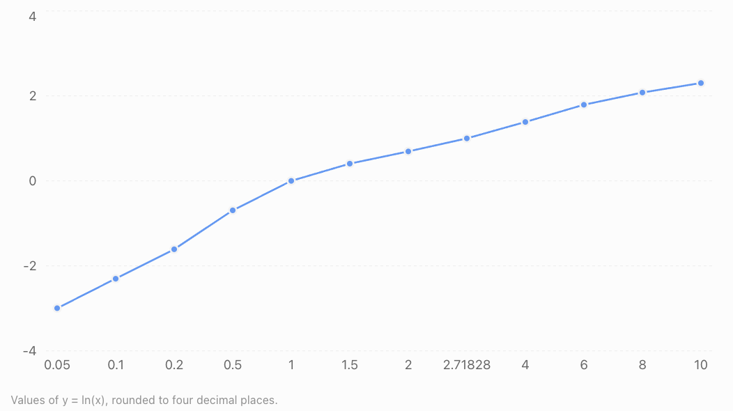
As x approaches zero from the right:
\[ \lim_{x\to0^+}\ln(x)=-\infty \]As x increases without bound:
\[ \lim_{x\to\infty}\ln(x)=\infty \]The function grows indefinitely, but very slowly.
Natural Logarithms and Inverse Functions
The natural logarithmic function and the natural exponential function are inverses.
This means that each function reverses the effect of the other.
The fundamental identities are:
\[ \boxed{\ln(e^x)=x} \]for every real x, and:
\[ \boxed{e^{\ln(x)}=x} \]for x > 0.
Reflection across y = x
Inverse functions have graphs that are reflections of each other across the line y = x.
For example:
-
The point (0, 1) on y = eˣ corresponds to (1, 0) on y = ln(x).
-
The point (1, e) on y = eˣ corresponds to (e, 1) on y = ln(x).
Inverse relationship between eˣ and ln(x)
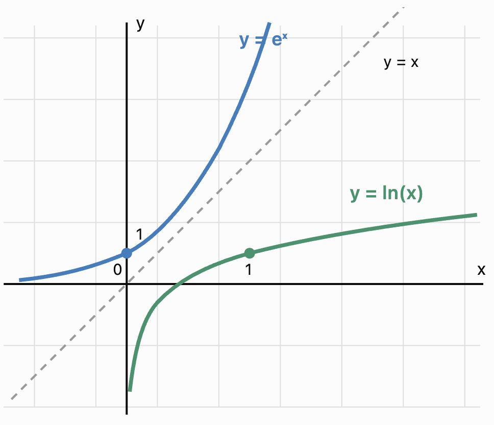 Conceptual illustration of the inverse relationship. The two curves are reflections across y = x; the drawing is schematic rather than a precision coordinate plot.
This inverse relationship is the foundation for solving natural exponential and logarithmic equations.
Properties of Natural Logarithms
Natural logarithms follow the same laws as logarithms with other valid bases.
These properties allow us to simplify expressions and solve equations.
For positive real numbers a and b, and any real number r:
Product property
\[ \boxed{\ln(ab)=\ln(a)+\ln(b)} \]The logarithm of a product equals the sum of the logarithms.
Example:
\[ \ln(2e)=\ln2+\ln e \]Since ln(e) = 1:
\[ \boxed{\ln(2e)=\ln2+1} \]Quotient property
\[ \boxed{\ln\left(\frac ab\right)=\ln(a)-\ln(b)} \]Example:
\[ \ln\left(\frac{e^3}{5}\right)=\ln(e^3)-\ln5 \]\[ \boxed{=3-\ln5} \]Power property
\[ \boxed{\ln(a^r)=r\ln(a)} \]Example:
\[ \ln(7^3)=3\ln7 \]Special identities
\[ \ln1=0 \]\[ \ln e=1 \]\[ \ln(e^x)=x \]\[ e^{\ln x}=x\quad(x>0) \]Worked Example 4: Expanding a Logarithm
Expand:
\[ \ln(5x^3) \]Assume x > 0.
Using the product property:
\[ \ln(5x^3)=\ln5+\ln(x^3) \]Apply the power property:
\[ \boxed{\ln(5x^3)=\ln5+3\ln x} \]Worked Example 5: Expanding a Quotient
Expand:
\[ \ln\left(\frac{3x^2}{y^4}\right) \]Assume x > 0 and y > 0.
Apply the quotient property:
\[ =\ln(3x^2)-\ln(y^4) \]Apply the product and power properties:
\[ \boxed{\ln3+2\ln x-4\ln y} \]For unrestricted nonzero real x and y, the fully general expression would instead use ln|x| and ln|y|.
Worked Example 6: Condensing Logarithms
Write as a single logarithm:
\[ 2\ln x+\ln3-\ln5 \]Assume x > 0.
Apply the power property:
\[ 2\ln x=\ln(x^2) \]Then combine:
\[ \ln(x^2)+\ln3=\ln(3x^2) \]Finally:
\[ \boxed{\ln\left(\frac{3x^2}{5}\right)} \]Solving Natural Logarithmic Equations
Natural logarithmic equations can be solved by converting between logarithmic and exponential forms.
The essential rule is:
\[ \ln(A)=b\iff A=e^b \]provided A > 0.
Worked Example 7: A Simple Logarithmic Equation
Solve:
\[ \ln x=3 \]Rewrite in exponential form:
\[ x=e^3 \]Therefore:
\[ \boxed{x\approx20.086} \]Worked Example 8: Logarithm of a Linear Expression
Solve:
\[ \ln(2x-1)=2 \]Step 1: Convert to exponential form.
\[ 2x-1=e^2 \]Step 2: Isolate x.
\[ 2x=e^2+1 \]\[ x=\frac{e^2+1}{2} \]Step 3: Evaluate.
\[ \boxed{x\approx4.195} \]Step 4: Check the domain.
The logarithm requires:
\[ 2x-1>0 \]\[ x>\frac12 \]Our solution satisfies the restriction.
Worked Example 9: Combining Logarithms
Solve:
\[ \ln x+\ln(x-3)=\ln10 \]Step 1: Identify domain restrictions.
\[ x>0,\qquad x-3>0 \]Therefore:
\[ x>3 \]Step 2: Combine the logarithms.
\[ \ln[x(x-3)]=\ln10 \]Step 3: Equate arguments.
\[ x(x-3)=10 \]\[ x^2-3x-10=0 \]Step 4: Factorise.
\[ (x-5)(x+2)=0 \]Therefore:
\[ x=5\quad\text{or}\quad x=-2 \]Step 5: Check the domain.
Since x > 3, the value −2 is invalid.
\[ \boxed{x=5} \]This illustrates why checking logarithmic domains is essential.
Solving Exponential Equations Using Natural Logarithms
Natural logarithms are also useful when the unknown appears in an exponent.
Worked Example 10: Solving an Exponential Equation
Solve:
\[ 5e^{0.4x}=30 \]Divide by 5:
\[ e^{0.4x}=6 \]Take natural logarithms:
\[ 0.4x=\ln6 \]Rearrange:
\[ x=\frac{\ln6}{0.4} \]\[ \boxed{x\approx4.479} \]Worked Example 11: Solving an Equation with a General Exponential Base
Solve:
\[ 3^x=20 \]Take natural logarithms of both sides:
\[ \ln(3^x)=\ln20 \]Apply the power property:
\[ x\ln3=\ln20 \]Therefore:
\[ x=\frac{\ln20}{\ln3} \]\[ \boxed{x\approx2.727} \]This method works with any positive exponential base other than 1.
Transformations of Natural Logarithmic Functions
The graph of y = ln(x) can be transformed through translations, reflections, and stretches.
A general form is:
\[ f(x)=a\ln[b(x-h)]+k \]where a and b are nonzero constants.
The parameters influence the graph's position and shape.
Function
Transformation
y = ln(x) + 3
Shift upward 3 units
y = ln(x − 2)
Shift right 2 units
y = ln(x + 4)
Shift left 4 units
y = −ln(x)
Reflection across the x-axis
y = 2ln(x)
Vertical stretch by factor 2
y = ln(−x)
Reflection across the y-axis
Worked Example 12: Analysing a Transformed Function
Consider:
\[ f(x)=2\ln(x-3)+1 \]Identify the domain, vertical asymptote, and transformations.
Transformations:
-
Shift right 3 units.
-
Vertical stretch by factor 2.
-
Shift upward 1 unit.
Domain:
The logarithm requires:
\[ x-3>0 \]\[ \boxed{x>3} \]Vertical asymptote:
\[ \boxed{x=3} \]Range:
All real numbers.
Finding the x-intercept
Set f(x) = 0.
\[ 2\ln(x-3)+1=0 \]\[ 2\ln(x-3)=-1 \]\[ \ln(x-3)=-\frac12 \]Convert to exponential form:
\[ x-3=e^{-1/2} \]\[ x=3+e^{-1/2} \]\[ \boxed{x\approx3.607} \]The graph crosses the x-axis at approximately (3.607, 0).
Natural Logarithms and Continuous Growth
One of the most important applications of natural logarithms is solving continuous growth and decay models.
The general model is:
\[ \boxed{Q(t)=Q_0e^{kt}} \]Where:
-
Q(t) = quantity at time t
-
Q₀ = initial quantity
-
k = continuous growth or decay rate
-
t = time
Natural logarithms allow us to solve for t when the initial and final quantities are known.
Starting with:
\[ Q=Q_0e^{kt} \]Divide by Q₀:
\[ \frac{Q}{Q_0}=e^{kt} \]Take natural logarithms:
\[ \ln\left(\frac{Q}{Q_0}\right)=kt \]Therefore:
\[ \boxed{t=\frac{\ln(Q/Q_0)}{k}} \]This formula is valid when Q and Q₀ are positive and k is nonzero.
Application: Population Growth
Worked Example 13: Time Required for Population Growth
A bacterial population initially contains 500 bacteria and grows continuously at 12% per hour.
How long will it take to reach 2,000 bacteria?
The model is:
\[ P(t)=500e^{0.12t} \]Set P(t) = 2000.
\[ 2000=500e^{0.12t} \]Divide by 500:
\[ 4=e^{0.12t} \]Take natural logarithms:
\[ \ln4=0.12t \]Rearrange:
\[ t=\frac{\ln4}{0.12} \]\[ t=\frac{1.386294}{0.12} \]\[ \boxed{t\approx11.55\text{ hours}} \]The population reaches 2,000 bacteria after approximately 11.55 hours under the model.
Application: Doubling Time
The doubling time is the time required for a growing quantity to become twice its initial value.
For:
\[ Q(t)=Q_0e^{kt} \]set:
\[ 2Q_0=Q_0e^{kt} \]Divide by Q₀:
\[ 2=e^{kt} \]Take natural logarithms:
\[ \ln2=kt \]Therefore:
\[ \boxed{t_d=\frac{\ln2}{k}} \]for k > 0.
Worked Example 14: Doubling Time
A population grows continuously at 5% per year.
Calculate its doubling time.
\[ t_d=\frac{\ln2}{0.05} \]\[ t_d=\frac{0.693147}{0.05} \]\[ \boxed{t_d\approx13.86\text{ years}} \]The population doubles approximately every 13.86 years if the continuous growth rate remains constant.
Application: Radioactive Decay
Natural logarithms are also essential for investigating radioactive decay.
The model is:
\[ N(t)=N_0e^{-\lambda t} \]Where λ is the positive decay constant.
Half-life formula
The half-life is the time required for the expected remaining quantity to decrease to half its original value.
\[ \boxed{t_{1/2}=\frac{\ln2}{\lambda}} \]Worked Example 15: Calculating Half-Life
A radioactive substance has a decay constant of 0.035 per year.
Calculate its half-life.
\[ t_{1/2}=\frac{\ln2}{0.035} \]\[ t_{1/2}=\frac{0.693147}{0.035} \]\[ \boxed{t_{1/2}\approx19.80\text{ years}} \]The substance has a half-life of approximately 19.8 years.
Application: Continuous Compound Interest
The continuous compound interest formula is:
\[ A=Pe^{rt} \]Where:
-
A = final amount
-
P = initial investment
-
r = annual interest rate
-
t = time in years
Natural logarithms allow us to calculate how long an investment needs to reach a target amount.
Worked Example 16: Investment Growth
An investment of $4,000 earns 6% annual interest compounded continuously.
How long will it take to reach $7,000?
Use:
\[ 7000=4000e^{0.06t} \]Divide by 4000:
\[ 1.75=e^{0.06t} \]Take natural logarithms:
\[ \ln1.75=0.06t \]Rearrange:
\[ t=\frac{\ln1.75}{0.06} \]\[ t=\frac{0.559616}{0.06} \]\[ \boxed{t\approx9.33\text{ years}} \]The investment reaches $7,000 after approximately 9.33 years.
Application: Natural Logarithms in Science
Natural logarithms appear in many scientific relationships.
Chemical Kinetics
First-order reactions can be analysed using logarithmic relationships. If concentration follows [A] = [A]₀e⁻ᵏᵗ, taking natural logarithms gives ln[A] = ln[A]₀ − kt.
Electrical Circuits
Capacitor discharge can be modelled exponentially. Natural logarithms help determine the time required for voltage to decrease to a specified level.
Biology
Natural logarithms help determine growth rates and doubling times for populations during approximately exponential growth phases.
Finance
Natural logarithms are used to calculate investment times, continuous rates of return, and other quantities in financial models.
Linearising Exponential Data
Natural logarithms can transform an exponential relationship into a linear relationship.
Suppose:
\[ y=Ae^{kx} \]where A > 0.
Take natural logarithms:
\[ \ln y=\ln(Ae^{kx}) \]Using logarithm properties:
\[ \ln y=\ln A+\ln(e^{kx}) \]Therefore:
\[ \boxed{\ln y=\ln A+kx} \]This is a straight-line equation in the variables x and ln
.
Its slope is k, and its intercept is ln(A).
Worked Example 17: Finding an Exponential Model
Suppose a quantity follows:
\[ y=Ae^{kx} \]and the data include:
-
At x = 0, y = 100.
-
At x = 4, y = 180.
Find A and k.
Step 1: Find A.
At x = 0:
\[ 100=Ae^0 \]\[ \boxed{A=100} \]Step 2: Substitute the second point.
\[ 180=100e^{4k} \]Divide by 100:
\[ 1.8=e^{4k} \]Take natural logarithms:
\[ \ln1.8=4k \]\[ k=\frac{\ln1.8}{4} \]\[ \boxed{k\approx0.14695} \]Therefore, the model is:
\[ \boxed{y=100e^{0.14695x}} \]The continuous growth rate is approximately 14.695% per unit of x.
This technique is useful in statistics because logarithmic transformations can reveal exponential patterns in data.
Common Mistakes
Mistake 1: Confusing ln(x) with log₁₀(x)
Natural logarithms use base e, while common logarithms use base 10.
Correction: Check which logarithm is required.
Mistake 2: Assuming ln(a + b) = ln(a) + ln(b)
This is false in general.
For example:
\[ \ln(2+3)=\ln5 \]but:
\[ \ln2+\ln3=\ln6 \]These are not equal.
Mistake 3: Taking the logarithm of zero or a negative number
The real-valued natural logarithm is defined only for positive inputs.
Correction: Check the domain before solving.
Mistake 4: Forgetting to check extraneous solutions
Algebraic manipulation may produce solutions that make a logarithm's argument zero or negative.
Correction: Substitute solutions into the original equation.
Mistake 5: Applying the power property incorrectly
The property is:
\[ \ln(x^n)=n\ln x \]for x > 0.
For even integer powers and negative x, absolute values may be required in the expanded expression.
Mistake 6: Confusing ln(eˣ) with eˡⁿ⁽ˣ⁾
Both inverse identities are useful, but the second requires x > 0.
Correction: Pay attention to domain restrictions.
Mistake 7: Using an incorrect growth-rate sign
A positive continuous rate represents growth, while a negative rate represents decay.
Correction: Interpret the sign of the exponent coefficient carefully.
Key Terms
-
Natural Logarithm: A logarithm with base e, written ln(x).
-
Euler's Number (e): An irrational constant approximately equal to 2.71828.
-
Logarithmic Function: A function involving the logarithm of a variable expression.
-
Inverse Function: A function that reverses the effect of another function.
-
Exponential Function: A function in which a variable appears in an exponent.
-
Domain: The set of allowable input values.
-
Range: The set of possible output values.
-
Vertical Asymptote: A vertical line approached by a graph as function values increase or decrease without bound.
-
Product Property: ln(ab) = ln(a) + ln(b).
-
Quotient Property: ln(a/b) = ln(a) − ln(b).
-
Power Property: ln(aʳ) = r ln(a), for a > 0.
-
Exponential Growth: Increase at a rate proportional to the current quantity.
-
Exponential Decay: Decrease at a rate proportional to the current quantity.
-
Continuous Growth Rate: The instantaneous relative growth rate in an exponential model.
-
Doubling Time: The time required for a growing quantity to double.
-
Half-Life: The time required for a decaying quantity to halve.
-
Continuous Compounding: The limiting form of increasingly frequent interest compounding.
-
Linearisation: Transforming a nonlinear relationship into a linear form.
-
Extraneous Solution: A solution produced during algebraic manipulation that does not satisfy the original equation.
Key Takeaways
-
Natural logarithms use base e and are written ln(x).
-
The natural logarithm is the inverse of the natural exponential function.
-
The identities ln(eˣ) = x and eˡⁿ⁽ˣ⁾ = x are fundamental.
-
The domain of ln(x) is x > 0, and its range is all real numbers.
-
The graph of y = ln(x) passes through (1, 0) and has a vertical asymptote at x = 0.
-
Natural logarithms follow product, quotient, and power properties.
-
Logarithmic equations must be solved with careful attention to domain restrictions.
-
Natural logarithms can solve equations where the unknown appears in an exponent.
-
Continuous growth and decay models can be rearranged using natural logarithms.
-
Doubling time and half-life formulas are derived using ln(2).
-
Natural logarithms are useful in finance, biology, chemistry, and physics.
-
Exponential relationships can be linearised by taking natural logarithms.
Check Your Understanding
Questions
Question 1: Exact Values
Evaluate:
a) ln(1)
b) ln(e⁴)
c) ln(e⁻²)
Question 2: Calculator Evaluation
Evaluate ln(12), correct to three decimal places.
Question 3: Expanding Logarithms
Expand:
\[ \ln(4x^3) \]Assume x > 0.
Question 4: Condensing Logarithms
Write as a single logarithm:
\[ 3\ln x+\ln2-\ln5 \]Assume x > 0.
Question 5: Solving a Simple Equation
Solve:
\[ \ln x=4 \]Question 6: Solving a Linear Logarithmic Equation
Solve:
\[ \ln(3x+2)=2 \]Question 7: Combining Logarithms
Solve:
\[ \ln x+\ln(x-2)=\ln8 \]Question 8: Exponential Equations
Solve:
\[ 4e^{0.5x}=20 \]Question 9: General Exponential Equations
Solve:
\[ 5^x=40 \]Question 10: Transformations
For:
\[ f(x)=\ln(x-4)+2 \]state the domain, vertical asymptote, and transformations relative to y = ln(x).
Question 11: Continuous Growth
A population starts at 600 and grows continuously at 9% per year.
How long will it take to reach 1,200?
Question 12: Continuous Interest
An investment of $5,000 earns 4% annual interest compounded continuously.
How long will it take to reach $8,000?
Question 13: Half-Life
A radioactive substance has a decay constant of 0.06 per day.
Calculate its half-life.
Question 14: Exponential Modelling
A quantity follows:
\[ y=Ae^{kx} \]Given that y = 50 when x = 0 and y = 100 when x = 5, determine A and k.
Fully Worked Answers
Answer 1: Exact Values
a)
\[ \boxed{\ln1=0} \]b)
\[ \boxed{\ln(e^4)=4} \]c)
\[ \boxed{\ln(e^{-2})=-2} \]Answer 2: Calculator Evaluation
\[ \ln12\approx2.48490665 \]To three decimal places:
\[ \boxed{2.485} \]Answer 3: Expanding Logarithms
\[ \ln(4x^3) \]Apply the product property:
\[ =\ln4+\ln(x^3) \]Apply the power property:
\[ \boxed{\ln4+3\ln x} \]Answer 4: Condensing Logarithms
\[ 3\ln x+\ln2-\ln5 \]Apply the power property:
\[ =\ln(x^3)+\ln2-\ln5 \]Combine:
\[ =\ln(2x^3)-\ln5 \]Therefore:
\[ \boxed{\ln\left(\frac{2x^3}{5}\right)} \]Answer 5: Solving a Simple Equation
\[ \ln x=4 \]Convert to exponential form:
\[ x=e^4 \]\[ \boxed{x\approx54.598} \]Answer 6: Solving a Linear Logarithmic Equation
\[ \ln(3x+2)=2 \]Convert to exponential form:
\[ 3x+2=e^2 \]Rearrange:
\[ 3x=e^2-2 \]\[ x=\frac{e^2-2}{3} \]\[ \boxed{x\approx1.796} \]The solution satisfies the domain condition 3x + 2 > 0.
Answer 7: Combining Logarithms
\[ \ln x+\ln(x-2)=\ln8 \]Domain restriction:
\[ x>2 \]Combine logarithms:
\[ \ln[x(x-2)]=\ln8 \]Equate arguments:
\[ x(x-2)=8 \]\[ x^2-2x-8=0 \]Factorise:
\[ (x-4)(x+2)=0 \]Therefore:
\[ x=4\quad\text{or}\quad x=-2 \]Only x = 4 satisfies x > 2.
\[ \boxed{x=4} \]Answer 8: Exponential Equations
\[ 4e^{0.5x}=20 \]Divide by 4:
\[ e^{0.5x}=5 \]Take natural logarithms:
\[ 0.5x=\ln5 \]\[ x=\frac{\ln5}{0.5} \]\[ \boxed{x\approx3.219} \]Answer 9: General Exponential Equations
\[ 5^x=40 \]Take natural logarithms:
\[ x\ln5=\ln40 \]\[ x=\frac{\ln40}{\ln5} \]\[ \boxed{x\approx2.292} \]Answer 10: Transformations
\[ f(x)=\ln(x-4)+2 \]The graph is shifted:
-
Right 4 units.
-
Upward 2 units.
The domain requires:
\[ x-4>0 \]\[ \boxed{x>4} \]The vertical asymptote is:
\[ \boxed{x=4} \]Answer 11: Continuous Growth
The model is:
\[ P(t)=600e^{0.09t} \]Set P(t) = 1200.
\[ 1200=600e^{0.09t} \]Divide by 600:
\[ 2=e^{0.09t} \]Take natural logarithms:
\[ \ln2=0.09t \]\[ t=\frac{\ln2}{0.09} \]\[ \boxed{t\approx7.70\text{ years}} \]Answer 12: Continuous Interest
\[ A=Pe^{rt} \]Substitute:
\[ 8000=5000e^{0.04t} \]Divide by 5000:
\[ 1.6=e^{0.04t} \]Take natural logarithms:
\[ \ln1.6=0.04t \]\[ t=\frac{\ln1.6}{0.04} \]\[ \boxed{t\approx11.75\text{ years}} \]Answer 13: Half-Life
Use:
\[ t_{1/2}=\frac{\ln2}{\lambda} \]Substitute λ = 0.06.
\[ t_{1/2}=\frac{0.693147}{0.06} \]\[ \boxed{t_{1/2}\approx11.55\text{ days}} \]Answer 14: Exponential Modelling
Given:
\[ y=Ae^{kx} \]At x = 0, y = 50.
\[ 50=Ae^0 \]\[ \boxed{A=50} \]At x = 5, y = 100.
\[ 100=50e^{5k} \]Divide by 50:
\[ 2=e^{5k} \]Take natural logarithms:
\[ \ln2=5k \]\[ k=\frac{\ln2}{5} \]\[ \boxed{k\approx0.1386} \]Therefore, the model is:
\[ \boxed{y=50e^{0.1386x}} \]The continuous growth rate is approximately 13.86% per unit of x.
Final Reflection
Natural logarithms are essential mathematical tools because they allow us to reverse exponential relationships.
They provide methods for solving equations, interpreting logarithmic graphs, simplifying expressions, and analysing processes that involve continuous growth or decay.
Their usefulness extends far beyond algebra. Natural logarithms help determine investment times, population doubling times, radioactive half-lives, and many other quantities in scientific and economic models.
The central relationship to remember is that natural logarithms and natural exponential functions are inverses:
\[ \boxed{\ln(e^x)=x} \]and:
\[ \boxed{e^{\ln x}=x\qquad(x>0)} \]Understanding these relationships provides a strong foundation for advanced algebra, calculus, statistics, and mathematical modelling.
-