Advanced Exponential and Logarithmic Models
1. Natural Exponential Functions
Learning outcomes
- I can explain the significance of the number .
- I can evaluate functions involving .
- I can compare natural exponential and other exponential functions.
- I can interpret natural growth models.
- I can apply natural exponential functions to practical situations.
Introduction
Imagine depositing money into a bank account that earns interest continuously. Imagine a population of bacteria growing at a rate proportional to its current size, or a radioactive substance gradually decreasing in mass.
These situations can be modelled using a special mathematical constant called Euler's number, represented by the symbol e.
The number e is one of the most important constants in mathematics. It appears in calculus, finance, biology, chemistry, physics, economics, and statistics.
Its approximate value is:
Like π, the number e is irrational. Its decimal expansion continues forever without repeating.
Exponential functions with base e are called natural exponential functions. They are particularly useful because they describe processes in which the rate of change is proportional to the quantity currently present.
In this lesson, we will investigate the significance of e, evaluate natural exponential functions, compare exponential models, interpret continuous growth and decay, and apply these ideas to practical problems.
Understanding Euler's Number
The constant e arises naturally when investigating continuous growth.
Consider an investment of $1 earning 100% annual interest.
If the interest is added once per year, the balance after one year is:
If interest is compounded twice per year:
If interest is compounded four times per year:
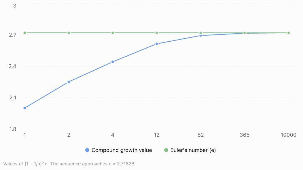
As the number of compounding periods increases, the balance approaches a particular value.
|
Compounding periods per year |
Final balance |
|---|---|
|
1 |
2.000000 |
|
2 |
2.250000 |
|
4 |
2.441406 |
|
12 |
2.613035 |
|
52 |
2.692597 |
|
365 |
2.714567 |
|
10,000 |
2.718146 |
|
Continuous limit |
2.718282 |
The limiting value is e.
Mathematically:
This is one way to define Euler's number.
Approaching Euler's number through compounding
Why is e significant?
The number e has several remarkable properties.
-
It is the natural base for continuous exponential growth and decay.
-
It appears in continuously compounded interest.
-
The function eˣ has a rate of change equal to its own value.
-
Its inverse function is the natural logarithm, ln(x).
-
It appears in probability distributions, differential equations, and many physical models.
The special relationship between eˣ and its rate of change makes natural exponential functions especially important in calculus.
The Natural Exponential Function
The basic natural exponential function is:
Here, e is the constant base and x is the exponent.
The function is defined for every real value of x.
Some useful values are:
|
x |
eˣ (approximately) |
|---|---|
|
−3 |
0.0498 |
|
−2 |
0.1353 |
|
−1 |
0.3679 |
|
0 |
1 |
|
1 |
2.7183 |
|
2 |
7.3891 |
|
3 |
20.0855 |
Properties of y = eˣ
-
Domain: All real numbers.
-
Range: y > 0.
-
y-intercept: (0, 1).
-
Horizontal asymptote: y = 0.
-
The function is continuous and strictly increasing.
-
It has no x-intercepts.
-
As x approaches positive infinity, eˣ increases without bound.
-
As x approaches negative infinity, eˣ approaches zero from above.
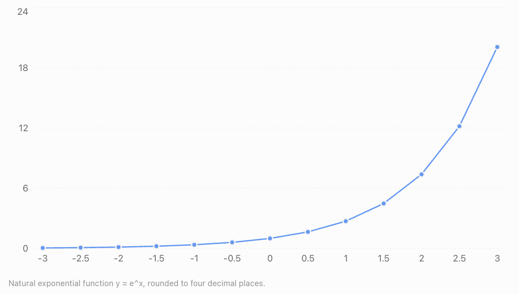
The graph passes through (0, 1) and increases increasingly rapidly as x becomes larger.
Although the curve approaches the x-axis for negative x-values, it never touches or crosses it.
Evaluating Natural Exponential Functions
To evaluate a natural exponential function, substitute the given value into the exponent and calculate.
Most scientific calculators have an eˣ function, often accessed using a secondary function key.
Worked Example 1: Evaluating eˣ
Evaluate:
\[ f(x)=e^{2x} \]when x = 1.5.
Step 1: Substitute the value.
\[ f(1.5)=e^{2(1.5)} \]Step 2: Simplify the exponent.
\[ f(1.5)=e^3 \]Step 3: Evaluate.
\[ \boxed{f(1.5)\approx20.086} \]Worked Example 2: Negative Exponents
Evaluate:
\[ g(x)=5e^{-0.4x} \]when x = 3.
Substitute:
\[ g(3)=5e^{-0.4(3)} \]\[ g(3)=5e^{-1.2} \]Since:
\[ e^{-1.2}\approx0.3010 \]Therefore:
\[ g(3)\approx5(0.3010) \]\[ \boxed{g(3)\approx1.506} \]A negative exponent does not produce a negative exponential value.
Instead:
\[ e^{-x}=\frac1{e^x} \]The result is always positive.
Worked Example 3: Evaluating a Transformed Function
Evaluate:
\[ h(x)=3e^{0.5x}-4 \]when x = 2.
\[ h(2)=3e^{0.5(2)}-4 \]\[ =3e^1-4 \]\[ \approx3(2.71828)-4 \]\[ \boxed{h(2)\approx4.155} \]The subtraction of 4 occurs after evaluating and multiplying the exponential term.
Laws of Exponents
Natural exponential functions follow the same exponent laws as other exponential functions.
For real numbers a and b:
Law
Expression
Product
eᵃ × eᵇ = eᵃ⁺ᵇ
Quotient
eᵃ / eᵇ = eᵃ⁻ᵇ
Power of a power
(eᵃ)ᵇ = eᵃᵇ
Zero exponent
e⁰ = 1
Negative exponent
e⁻ᵃ = 1/eᵃ
Worked Example 4: Simplifying Exponential Expressions
Simplify:
\[ \frac{e^{3x}e^{2x}}{e^x} \]Combine the terms in the numerator.
\[ e^{3x}e^{2x}=e^{5x} \]Now divide.
\[ \frac{e^{5x}}{e^x}=e^{5x-x} \]\[ \boxed{e^{4x}} \]These laws are useful when simplifying exponential models and solving equations.
Comparing Natural Exponential Functions with Other Exponential Functions
A general exponential function has the form:
\[ f(x)=a^x \]where a > 0 and a ≠ 1.
A natural exponential function uses the specific base e:
\[ f(x)=e^x \]Consider three functions:
\[ f(x)=2^x \]\[ g(x)=e^x \]\[ h(x)=3^x \]All three pass through (0, 1), because any positive base raised to the power zero equals 1.
For positive x, larger bases produce larger values.
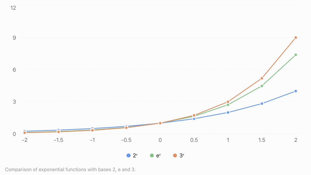
Important comparison
Property
2ˣ
eˣ
3ˣ
Base
2
Approximately 2.718
3
y-intercept
1
1
1
Domain
All real numbers
All real numbers
All real numbers
Range
Positive real numbers
Positive real numbers
Positive real numbers
Behaviour
Growth
Growth
Growth
Derivative
2ˣ ln(2)
eˣ
3ˣ ln(3)
The derivative property is what makes e especially useful.
For any positive base a:
\[ \frac{d}{dx}a^x=a^x\ln(a) \]For a = e:
\[ \ln(e)=1 \]Therefore:
\[ \boxed{\frac{d}{dx}e^x=e^x} \]The function eˣ is its own derivative.
This means its instantaneous rate of change at any point is equal to its value at that point.
Natural Exponential Growth and Decay
Many real-world processes change at a rate proportional to the amount currently present.
These can be modelled by:
\[ \boxed{Q(t)=Q_0e^{kt}} \]Where:
-
Q(t) = quantity at time t
-
Q₀ = initial quantity
-
k = continuous growth or decay rate
-
t = time
Exponential growth
When k > 0:
\[ Q(t)=Q_0e^{kt} \]The quantity increases over time.
Examples include idealised population growth, continuously compounded investments, and early-stage microbial growth under favourable conditions.
Exponential decay
When k < 0:
\[ Q(t)=Q_0e^{kt} \]The quantity decreases over time.
Examples include radioactive decay, drug elimination under certain conditions, and the discharge of a capacitor.
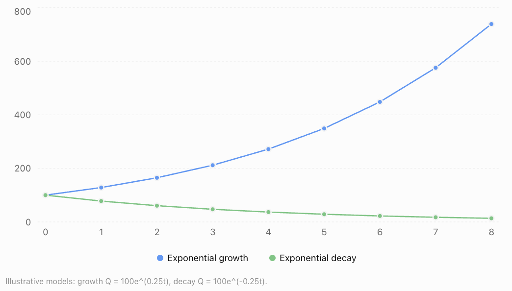
Both models begin at 100, but their values move in opposite directions.
Interpreting the Continuous Growth Rate
The parameter k represents the continuous relative rate of change.
For the model:
\[ Q(t)=Q_0e^{kt} \]the derivative is:
\[ \frac{dQ}{dt}=kQ \]Therefore:
\[ \frac1Q\frac{dQ}{dt}=k \]This shows that the instantaneous rate of change is proportional to the quantity present.
Continuous rate versus percentage growth per period
Suppose:
\[ Q(t)=Q_0e^{0.06t} \]The continuous growth rate is 6% per unit of time.
However, the actual percentage increase over one time unit is:
\[ (e^{0.06}-1)\times100\% \]\[ \approx6.184\% \]Thus, a continuous growth rate of 6% is not exactly the same as a 6% increase per year.
Conversely, if a quantity grows by exactly 6% each year:
\[ Q(t)=Q_0(1.06)^t \]This can be rewritten as:
\[ Q(t)=Q_0e^{t\ln(1.06)} \]The equivalent continuous rate is:
\[ k=\ln(1.06)\approx0.05827 \]or approximately 5.827% per year.
This distinction is important when comparing exponential models.
Converting Between Exponential Forms
Any exponential function with a positive base can be expressed using e.
The key identity is:
\[ \boxed{a^x=e^{x\ln(a)}} \]For example:
\[ 2^x=e^{x\ln2} \]Since ln(2) ≈ 0.6931:
\[ 2^x\approx e^{0.6931x} \]Similarly:
\[ 1.08^t=e^{t\ln(1.08)} \]\[ \approx e^{0.07696t} \]This allows us to compare discrete percentage growth models with continuous exponential growth models.
Continuous Compound Interest
Natural exponential functions are especially useful in financial mathematics.
When interest is compounded continuously:
\[ \boxed{A=Pe^{rt}} \]Where:
-
A = final amount
-
P = principal or initial investment
-
r = annual interest rate as a decimal
-
t = time in years
Worked Example 5: Continuous Interest
An investment of $5,000 earns 4% annual interest, compounded continuously.
Calculate the value after 6 years.
Step 1: Identify the variables.
P = 5000
r = 0.04
t = 6
Step 2: Substitute.
\[ A=5000e^{0.04(6)} \]\[ A=5000e^{0.24} \]Step 3: Evaluate.
\[ A\approx5000(1.271249) \]\[ \boxed{A\approx\$6,356.25} \]The investment grows to approximately $6,356.25.
The interest earned is:
\[ 6356.25-5000=\boxed{\$1,356.25} \]Comparing continuous and annual compounding
With annual compounding:
\[ A=P(1+r)^t \]\[ A=5000(1.04)^6 \]\[ A\approx\$6,326.60 \]Continuous compounding produces a slightly larger amount because interest is effectively added more frequently.
Population Growth
Natural exponential functions can model populations that grow at rates proportional to their current size.
Worked Example 6: Bacterial Growth
A bacterial culture initially contains 800 bacteria.
Its population grows at a continuous rate of 18% per hour.
Estimate the population after 5 hours.
The model is:
\[ P(t)=800e^{0.18t} \]Substitute t = 5.
\[ P(5)=800e^{0.18(5)} \]\[ P(5)=800e^{0.9} \]Since:
\[ e^{0.9}\approx2.4596 \]\[ P(5)\approx800(2.4596) \]\[ \boxed{P(5)\approx1968} \]The predicted population is approximately 1,968 bacteria.
Limitations of the model
Exponential population growth assumes the relative growth rate remains constant.
In real biological systems, nutrients, space, waste accumulation, and competition can limit growth.
Consequently, exponential models may be appropriate only during certain stages of population development.
Exponential Decay and Radioactive Half-Life
Radioactive substances decay at rates proportional to the number of radioactive nuclei remaining.
A common model is:
\[ N(t)=N_0e^{-\lambda t} \]Where:
-
N(t) = number of radioactive nuclei remaining
-
N₀ = initial number
-
λ = positive decay constant
-
t = time
Half-life
The half-life is the time required for the expected remaining quantity to decrease to half its initial value.
At the half-life:
\[ \frac{N_0}{2}=N_0e^{-\lambda t} \]Divide by N₀.
\[ \frac12=e^{-\lambda t} \]Take natural logarithms.
\[ \ln\left(\frac12\right)=-\lambda t \]Since ln(1/2) = −ln(2):
\[ \boxed{t_{1/2}=\frac{\ln2}{\lambda}} \]Worked Example 7: Radioactive Decay
A radioactive substance has a decay constant of 0.12 per day.
Calculate its half-life.
\[ t_{1/2}=\frac{\ln2}{0.12} \]\[ t_{1/2}=\frac{0.693147}{0.12} \]\[ \boxed{t_{1/2}\approx5.78\text{ days}} \]The expected remaining quantity halves approximately every 5.78 days.
Doubling Time
For exponential growth:
\[ Q(t)=Q_0e^{kt} \]where k > 0.
The doubling time is the time required for the quantity to become twice its initial value.
Set:
\[ 2Q_0=Q_0e^{kt} \]Divide by Q₀.
\[ 2=e^{kt} \]Take natural logarithms.
\[ \ln2=kt \]Therefore:
\[ \boxed{t_d=\frac{\ln2}{k}} \]Worked Example 8: Doubling Time
A population grows continuously at 3.5% per year.
Calculate its doubling time.
\[ t_d=\frac{\ln2}{0.035} \]\[ t_d=\frac{0.693147}{0.035} \]\[ \boxed{t_d\approx19.80\text{ years}} \]The population doubles approximately every 19.8 years if the continuous growth rate remains constant.
Solving Natural Exponential Equations
The natural logarithm, ln(x), is the inverse of the natural exponential function.
The identities are:
\[ \ln(e^x)=x \]and, for x > 0:
\[ e^{\ln x}=x \]These allow us to solve equations containing e.
Worked Example 9: Solving for an Exponent
Solve:
\[ e^{2x}=15 \]Take natural logarithms of both sides.
\[ \ln(e^{2x})=\ln15 \]\[ 2x=\ln15 \]\[ x=\frac{\ln15}{2} \]\[ \boxed{x\approx1.354} \]Worked Example 10: Finding a Time
A substance decays according to:
\[ M(t)=200e^{-0.08t} \]Find when the mass reaches 50 g.
Set M(t) = 50.
\[ 50=200e^{-0.08t} \]Divide by 200.
\[ 0.25=e^{-0.08t} \]Take natural logarithms.
\[ \ln0.25=-0.08t \]Rearrange.
\[ t=\frac{\ln0.25}{-0.08} \]\[ \boxed{t\approx17.33} \]The mass reaches 50 g after approximately 17.33 time units.
Transformations of Natural Exponential Functions
The basic function y = eˣ can be transformed.
A general form is:
\[ f(x)=Ae^{k(x-h)}+d \]Where:
-
A controls vertical scaling and reflection.
-
k controls horizontal scaling and whether the function grows or decays as x increases.
-
h shifts the graph horizontally.
-
d shifts the graph vertically.
For A > 0:
Function
Transformation
y = 3eˣ
Vertical stretch by factor 3
y = eˣ + 2
Shift upward 2 units
y = eˣ⁻²
Shift right 2 units
y = −eˣ
Reflection across the x-axis
y = e⁻ˣ
Reflection across the y-axis
Worked Example 11: Identifying Transformations
Consider:
\[ f(x)=2e^{x-3}+4 \]Relative to y = eˣ:
-
The graph is stretched vertically by a factor of 2.
-
It is shifted 3 units to the right.
-
It is shifted 4 units upward.
Its horizontal asymptote is:
\[ \boxed{y=4} \]Its range is:
\[ \boxed{y>4} \]The domain remains all real numbers.
Real-World Applications
Finance
Continuously compounded interest models idealised investment growth. Natural exponential functions also appear in discounting and financial mathematics.
Biology
Exponential models describe some stages of bacterial reproduction and population growth when resources are sufficiently abundant.
Medicine
Under suitable assumptions, first-order drug elimination can be represented using exponential decay, helping researchers study how drug concentrations change over time.
Physics and Engineering
Natural exponential functions model capacitor charging and discharging, radioactive decay, and certain cooling processes.
Common Mistakes
Mistake 1: Treating e as a variable
The symbol e represents a fixed mathematical constant.
Correction: Remember that e ≈ 2.71828.
Mistake 2: Confusing eˣ with e × x
Exponential notation means e raised to the power x, not multiplication.
For example:
e² ≈ 7.389, while 2e ≈ 5.437.
Mistake 3: Assuming a negative exponent produces a negative result
The expression e⁻ˣ is always positive.
Correction: Use e⁻ˣ = 1/eˣ.
Mistake 4: Confusing continuous and discrete growth rates
A continuous growth rate of 5% per year does not correspond to exactly 5% growth over one year.
Correction: Use eᵏ − 1 to find the effective growth factor over one time unit.
Mistake 5: Using a positive rate for exponential decay
In Q = Q₀eᵏᵗ, a positive k produces growth.
Correction: Use k < 0 for decay.
Mistake 6: Forgetting to use natural logarithms when solving for time
An equation such as e⁰·²ᵗ = 5 cannot be solved by ordinary algebra alone.
Correction: Apply ln to both sides.
Mistake 7: Applying exponential models indefinitely
Real populations and economic processes often face limits or changing conditions.
Correction: Evaluate whether the constant relative growth assumption remains realistic.
Key Terms
-
Euler's Number (e): An irrational mathematical constant approximately equal to 2.71828.
-
Natural Exponential Function: An exponential function with base e.
-
Exponential Growth: Growth at a rate proportional to the current quantity.
-
Exponential Decay: Decrease at a rate proportional to the current quantity.
-
Continuous Growth Rate: The instantaneous relative rate of growth in an exponential model.
-
Continuous Compounding: Interest calculation using the limiting process of increasingly frequent compounding.
-
Initial Value: The quantity present when time equals zero.
-
Growth Constant: The positive parameter k in Q = Q₀eᵏᵗ.
-
Decay Constant: A positive parameter λ used in Q = Q₀e⁻λᵗ.
-
Doubling Time: The time required for a growing quantity to double.
-
Half-Life: The time required for a decaying quantity to halve.
-
Natural Logarithm: A logarithm with base e, written ln(x).
-
Horizontal Asymptote: A horizontal line approached by a graph as x moves toward positive or negative infinity.
-
Irrational Number: A number that cannot be expressed as a ratio of two integers.
-
Continuous Model: A mathematical model defined over continuous values of the independent variable.
-
Exponential Equation: An equation containing a variable in an exponent.
Key Takeaways
-
Euler's number e is approximately 2.71828 and arises naturally in continuous growth processes.
-
The natural exponential function is f(x) = eˣ.
-
The domain of eˣ is all real numbers, and its range is positive real numbers.
-
Natural exponential functions follow the usual exponent laws.
-
The derivative of eˣ is eˣ, making it especially important in calculus.
-
General exponential functions can be rewritten using base e.
-
The model Q = Q₀eᵏᵗ describes continuous exponential growth or decay.
-
Positive k produces growth, while negative k produces decay.
-
The continuous growth rate is not exactly equal to the percentage increase over one full time period.
-
Continuous compound interest is modelled by A = Peʳᵗ.
-
Doubling time is ln(2)/k for k > 0.
-
Half-life is ln(2)/λ for a positive decay constant λ.
-
Natural logarithms are used to solve equations containing variable exponents.
-
Natural exponential models are useful in finance, biology, medicine, physics, and engineering.
Check Your Understanding
Questions
Question 1: Euler's Number
State the approximate value of e to four decimal places and explain one reason why it is important.
Question 2: Evaluating Functions
Evaluate:
\[ f(x)=e^{3x} \]when x = 2.
Question 3: Negative Exponents
Evaluate:
\[ g(x)=4e^{-0.5x} \]when x = 4.
Question 4: Exponent Laws
Simplify:
\[ \frac{e^{5x}e^{2x}}{e^{3x}} \]Question 5: Comparing Functions
Explain one similarity and one difference between y = 2ˣ and y = eˣ.
Question 6: Continuous Growth
A population initially contains 1,200 organisms and grows continuously at 7% per year.
Write a model and estimate the population after 5 years.
Question 7: Continuous Interest
An investment of $8,000 earns 3.5% annual interest compounded continuously.
Calculate its value after 10 years.
Question 8: Exponential Decay
A substance initially has a mass of 500 g and decays according to:
\[ M(t)=500e^{-0.15t} \]Calculate its mass after 6 time units.
Question 9: Doubling Time
A population grows continuously at 4% per year.
Calculate its doubling time.
Question 10: Half-Life
A radioactive substance has a decay constant of 0.08 per day.
Calculate its half-life.
Question 11: Solving Exponential Equations
Solve:
\[ e^{0.3x}=10 \]Question 12: Converting Exponential Forms
Rewrite:
\[ P(t)=500(1.06)^t \]in the form:
\[ P(t)=500e^{kt} \]Give k to four decimal places.
Question 13: Transformations
Describe the transformations of:
\[ f(x)=3e^{x-2}-5 \]relative to y = eˣ.
State the horizontal asymptote.
Question 14: Interpreting a Model
A quantity follows:
\[ Q(t)=250e^{-0.06t} \]Explain the meaning of 250 and −0.06, and state whether the model represents growth or decay.
Fully Worked Answers
Answer 1: Euler's Number
Euler's number is:
\[ \boxed{e\approx2.7183} \]It is important because it is the natural base for continuous exponential growth and decay.
The function eˣ also has the special property that its derivative equals itself.
Answer 2: Evaluating Functions
Given:
\[ f(x)=e^{3x} \]Substitute x = 2.
\[ f(2)=e^{3(2)}=e^6 \]\[ \boxed{f(2)\approx403.429} \]Answer 3: Negative Exponents
\[ g(x)=4e^{-0.5x} \]Substitute x = 4.
\[ g(4)=4e^{-0.5(4)} \]\[ =4e^{-2} \]\[ \approx4(0.135335) \]\[ \boxed{g(4)\approx0.5413} \]Answer 4: Exponent Laws
\[ \frac{e^{5x}e^{2x}}{e^{3x}} \]Combine the numerator.
\[ =\frac{e^{7x}}{e^{3x}} \]Subtract exponents.
\[ =e^{7x-3x} \]\[ \boxed{e^{4x}} \]Answer 5: Comparing Functions
Both functions are exponential growth functions with positive bases greater than 1.
Both pass through (0, 1), have a domain of all real numbers, and have a range of positive real numbers.
However, eˣ grows faster than 2ˣ for positive x because e > 2.
The function eˣ also has the special property that its derivative equals itself.
Answer 6: Continuous Growth
The initial population is 1,200.
The continuous growth rate is 7%, so k = 0.07.
The model is:
\[ P(t)=1200e^{0.07t} \]After 5 years:
\[ P(5)=1200e^{0.35} \]\[ \approx1200(1.419068) \]\[ \boxed{P(5)\approx1703} \]The predicted population is approximately 1,703 organisms.
Answer 7: Continuous Interest
Use:
\[ A=Pe^{rt} \]Substitute P = 8000, r = 0.035, and t = 10.
\[ A=8000e^{0.035(10)} \]\[ A=8000e^{0.35} \]\[ \approx8000(1.419068) \]\[ \boxed{A\approx\$11,352.54} \]Answer 8: Exponential Decay
\[ M(t)=500e^{-0.15t} \]Substitute t = 6.
\[ M(6)=500e^{-0.9} \]\[ \approx500(0.406570) \]\[ \boxed{M(6)\approx203.28\text{ g}} \]Answer 9: Doubling Time
The continuous growth rate is k = 0.04.
\[ t_d=\frac{\ln2}{0.04} \]\[ t_d=\frac{0.693147}{0.04} \]\[ \boxed{t_d\approx17.33\text{ years}} \]Answer 10: Half-Life
The decay constant is λ = 0.08.
\[ t_{1/2}=\frac{\ln2}{0.08} \]\[ t_{1/2}=\frac{0.693147}{0.08} \]\[ \boxed{t_{1/2}\approx8.66\text{ days}} \]Answer 11: Solving Exponential Equations
\[ e^{0.3x}=10 \]Take natural logarithms.
\[ 0.3x=\ln10 \]Divide by 0.3.
\[ x=\frac{\ln10}{0.3} \]\[ \boxed{x\approx7.675} \]Answer 12: Converting Exponential Forms
Given:
\[ P(t)=500(1.06)^t \]Use:
\[ a^t=e^{t\ln a} \]Therefore:
\[ P(t)=500e^{t\ln(1.06)} \]Since:
\[ \ln(1.06)\approx0.05827 \]The model becomes:
\[ \boxed{P(t)\approx500e^{0.0583t}} \]The equivalent continuous growth rate is approximately 5.827% per time unit.
Answer 13: Transformations
The function is:
\[ f(x)=3e^{x-2}-5 \]Relative to y = eˣ:
-
Vertical stretch by factor 3.
-
Shift right 2 units.
-
Shift downward 5 units.
The horizontal asymptote is:
\[ \boxed{y=-5} \]Answer 14: Interpreting a Model
The model is:
\[ Q(t)=250e^{-0.06t} \]The initial quantity is 250 because:
\[ Q(0)=250e^0=250 \]The coefficient −0.06 indicates a continuous decay rate of 6% per time unit.
Because the exponent coefficient is negative, the model represents exponential decay.
The quantity decreases over time while remaining positive.
Final Reflection
Natural exponential functions provide a powerful way to understand processes that change continuously.
Their importance comes from the special properties of Euler's number and the fact that the rate of change of eˣ is equal to its current value.
This makes natural exponential functions especially useful when modelling growth and decay in real-world situations.
The central idea is that when the rate of change of a quantity is proportional to the quantity itself, a natural exponential model is often appropriate.
Understanding this principle creates an important connection between algebra, calculus, statistics, and the mathematical modelling of the natural world.
-