Exponential Function
5. Applications of Exponential Functions
Learning outcomes
- I can model compound interest.
- I can model population growth.
- I can model radioactive decay.
- I can analyse depreciation problems.
- I can solve authentic applications of exponential change.
Applications of Exponential Functions
Exponential functions are useful whenever a quantity changes by the same percentage or multiplication factor over equal intervals of time. They allow us to model situations in finance, biology, physics, economics, technology, and many other fields.
Common applications include:
- compound interest
- population growth
- radioactive decay
- depreciation
- bacterial growth
- medication concentration
- inflation
- spread of information or disease
- cooling and other decay processes
The important skill is not simply substituting numbers into an equation. We need to decide which exponential model fits the situation, interpret its parameters, perform the calculation, and decide whether the answer makes sense.


Recognizing an Exponential Situation
A situation may be exponential if a quantity changes by a constant percentage rather than a constant amount.
For example, suppose an investment increases by 5% each year.
If it begins at $1,000:
Year 0: $1,000
Year 1: $1,050
Year 2: $1,102.50
Year 3: $1,157.63
The amount added each year changes, but the percentage remains 5%.
This is exponential growth.
A general exponential model can be written as:
A = A₀bᵗ
where:
- A = amount after time t
- A₀ = initial amount
- b = growth or decay factor
- t = number of time periods
For growth:
b > 1
For decay:
0 < b < 1
Compound Interest
Compound interest occurs when interest is calculated not only on the original amount invested but also on interest that has already been earned.
This creates exponential growth.
For annual compounding, a basic model is:
A = P(1 + r)ᵗ
where:
- A = final amount
- P = principal or initial investment
- r = annual interest rate as a decimal
- t = number of years
The expression 1 + r is the growth factor.
For example, an interest rate of 6% gives:
r = 0.06
Growth factor:
1 + 0.06 = 1.06
So the investment is multiplied by 1.06 each year.
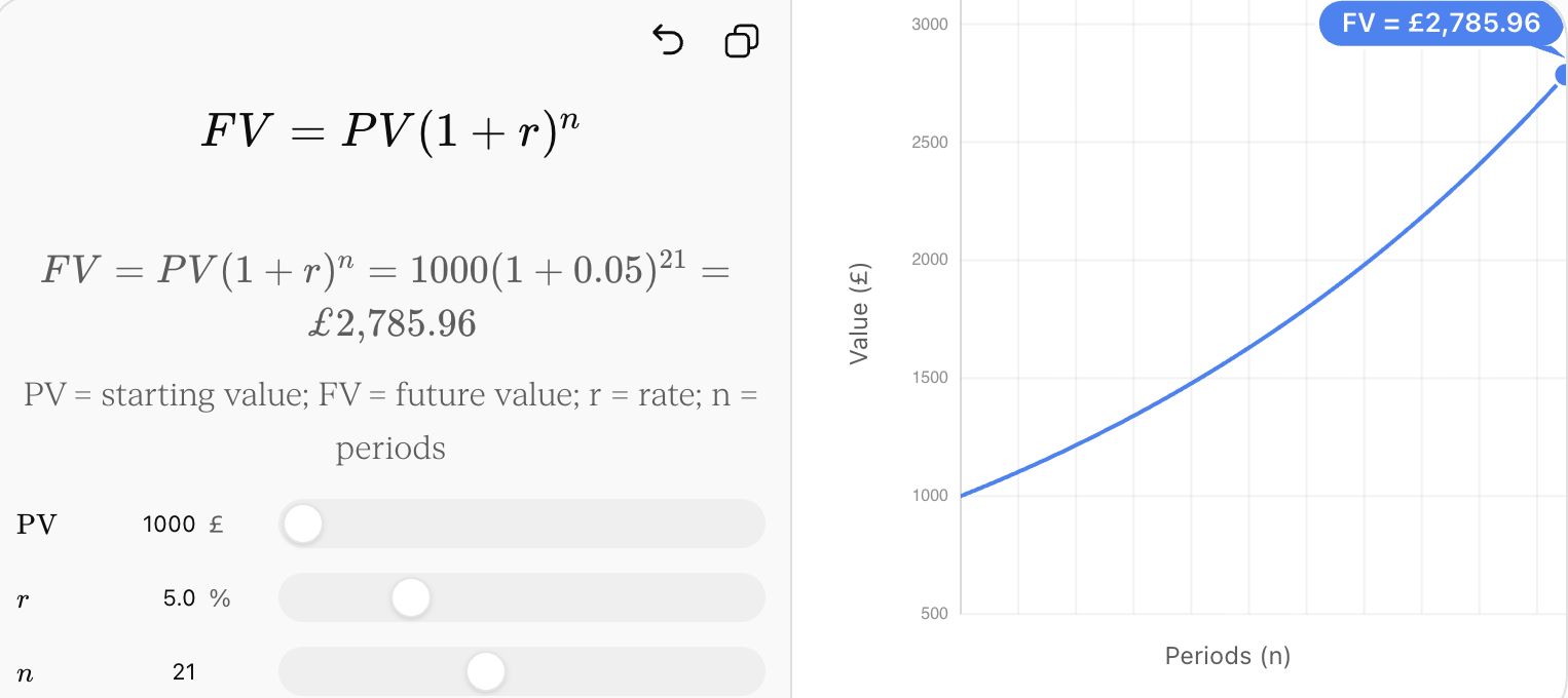
The effect of repeated compounding can be explored here:
Worked Example: Compound Interest
Suppose $5,000 is invested at 4% annual compound interest for 8 years.
Identify the values:
P = 5000
r = 0.04
t = 8
Substitute:
A = 5000(1.04)⁸
A ≈ 6842.85
The investment will be worth approximately:
$6,842.85
The amount of interest earned is:
6842.85 − 5000 = 1842.85
Therefore, approximately $1,842.85 in interest was earned.
Compound Interest More Than Once Per Year
Interest may be compounded several times each year.
A more general formula is:
A = P(1 + r/n)^(nt)
where:
- P = principal
- r = annual interest rate
- n = number of compounding periods per year
- t = number of years
For example:
- annually → n = 1
- semi-annually → n = 2
- quarterly → n = 4
- monthly → n = 12
Example
$2,000 is invested at 6% annual interest compounded monthly for 5 years.
P = 2000
r = 0.06
n = 12
t = 5
A = 2000(1 + 0.06/12)^(12 × 5)
A = 2000(1.005)⁶⁰
A ≈ 2697.70
The account will contain approximately $2,697.70.


Population Growth
Populations can sometimes be modelled using exponential functions when they increase by approximately the same percentage during each time interval.
A simple population model is:
P = P₀(1 + r)ᵗ
where:
- P = future population
- P₀ = initial population
- r = growth rate
- t = time
Worked Example
A town has 25,000 people and grows by 3% each year. Estimate its population after 10 years.
P₀ = 25000
r = 0.03
t = 10
P = 25000(1.03)¹⁰
P ≈ 33,598
The model predicts approximately:
33,598 people
Interpreting a Population Model
Suppose:
P = 4800(1.025)ᵗ
We can interpret the model directly.
4800 represents the initial population.
1.025 is the growth factor.
Therefore:
1.025 − 1 = 0.025
The growth rate is:
2.5% per time period
If t is measured in years, the population increases by 2.5% per year.
When Exponential Population Growth Becomes Unrealistic
Exponential models assume that the same proportional growth can continue.
Real populations eventually encounter limits such as:
- available food
- water
- space
- disease
- competition
- predation
- habitat availability
As a result, exponential growth may be useful over a limited period but unrealistic over very long periods.
In ecology, a logistic model may be more appropriate when growth slows as the population approaches the environment's carrying capacity.
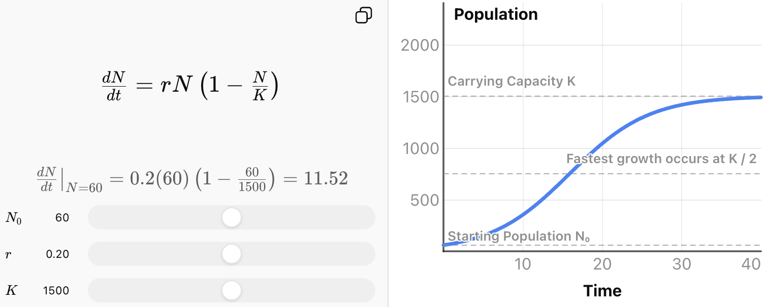
This is an important lesson about mathematical modelling: a mathematically correct calculation is only useful if the model itself is appropriate.


Radioactive Decay
Radioactive substances contain unstable nuclei that decay over time.
Although individual radioactive nuclei decay unpredictably, a large sample follows a predictable exponential pattern.
A decay model can be written as:
N = N₀(1 − r)ᵗ
where:
- N = amount remaining
- N₀ = initial amount
- r = decay rate
- t = time
Radioactive decay is often described using half-life.
Half-Life
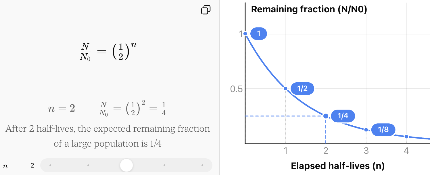
The half-life of a radioactive substance is the time required for half of the radioactive nuclei in a large sample to decay.
A half-life model can be written as:
N = N₀(1/2)^(t/h)
where:
- N = amount remaining
- N₀ = initial amount
- t = elapsed time
- h = half-life
Each complete half-life multiplies the amount by 1/2.
Worked Example: Radioactive Decay
A radioactive isotope has a half-life of 6 years. A sample initially contains 320 mg.
How much remains after 18 years?
First determine the number of half-lives:
18 ÷ 6 = 3 half-lives
Now repeatedly halve the quantity:
320 → 160 → 80 → 40
Therefore:
40 mg remains.
We can also use the equation:
N = 320(1/2)^(18/6)
N = 320(1/2)³
N = 320 × 1/8
N = 40 mg
Radioactive Decay Never Simply Subtracts the Same Amount
Suppose a 400 g sample has a half-life of 5 years.
After 5 years:
400 → 200 g
After another 5 years:
200 → 100 g
After another 5 years:
100 → 50 g
The amount lost is different each time:
- first interval: 200 g lost
- second interval: 100 g lost
- third interval: 50 g lost
But the fraction lost remains constant.
This is why radioactive decay is exponential rather than linear.


Depreciation
Depreciation describes a decrease in the value of an asset over time.
Cars, computers, machinery, phones, and other equipment may lose a percentage of their value each year.
A common exponential depreciation model is:
V = V₀(1 − r)ᵗ
where:
- V = value after time t
- V₀ = original value
- r = depreciation rate
- t = number of time periods
Worked Example: Vehicle Depreciation
A car costs $36,000 and depreciates by 18% each year.
Find its estimated value after 4 years.
Initial value:
V₀ = 36000
Depreciation rate:
r = 0.18
Decay factor:
1 − 0.18 = 0.82
Model:
V = 36000(0.82)ᵗ
After four years:
V = 36000(0.82)⁴
V ≈ 16,874.77
The model predicts a value of approximately:
$16,874.77
Interpreting Depreciation Correctly
An 18% depreciation rate does not mean that the asset loses 18% of its original value every year.
Instead, it loses 18% of its current value.
For the $36,000 car:
First year:
36000 × 0.82 = 29520
Second year:
29520 × 0.82 = 24206.40
The dollar amount lost decreases even though the percentage remains 18%.
This repeated proportional decrease creates exponential decay.


Comparing Common Exponential Applications
| Application | Growth or decay? | Typical model |
|---|---|---|
| Compound interest | Growth | A = P(1 + r)ᵗ |
| Population increase | Growth | P = P₀(1 + r)ᵗ |
| Radioactive decay | Decay | N = N₀(1/2)^(t/h) |
| Percentage depreciation | Decay | V = V₀(1 − r)ᵗ |
Although the contexts are very different, the mathematical structure is similar.
Each model contains:
initial amount × repeated multiplication
Recognizing this common structure makes exponential applications much easier to solve.
Determining the Rate from an Equation
Sometimes the model is already provided.
Consider:
P = 8000(1.06)ᵗ
The growth factor is:
1.06
Therefore:
1.06 − 1 = 0.06
The growth rate is:
6%
Now consider:
V = 24000(0.87)ᵗ
The decay factor is:
0.87
Therefore:
1 − 0.87 = 0.13
The depreciation rate is:
13%
Building a Model from a Description
Suppose a problem states:
A wildlife population begins at 12,500 and decreases by 4% each year.
Identify the initial value:
P₀ = 12500
Convert the rate:
4% = 0.04
Since this is decay:
1 − 0.04 = 0.96
Therefore:
P = 12500(0.96)ᵗ
Once the model has been created, it can be used to predict the population at different times.
Solving an Authentic Application
Suppose a company purchases a piece of equipment for $85,000. The equipment loses 12% of its value each year.
The company plans to sell it after 7 years.
Build the Model
Initial value:
V₀ = 85000
Depreciation rate:
r = 0.12
Decay factor:
1 − 0.12 = 0.88
Therefore:
V = 85000(0.88)ᵗ
Calculate the Value After 7 Years
V = 85000(0.88)⁷
V ≈ 34,738
The model predicts that the equipment will be worth approximately $34,738 after seven years.
Interpret the Result
The model assumes that the equipment continues to lose 12% of its current value every year.
In reality, its resale value could also depend on:
- condition
- maintenance
- technological changes
- market demand
- inflation
This illustrates the difference between a mathematical model and the real system it represents.
A Strategy for Exponential Application Problems
When solving a practical problem, first identify the initial amount, then decide whether the situation involves growth or decay. Convert the percentage to a decimal and determine the multiplication factor.
For growth:
factor = 1 + r
For decay:
factor = 1 − r
Then write the exponential model, substitute the required time, calculate, and interpret the answer using appropriate units.
Finally, ask:
Does the answer make sense in the context of the problem?
Checking Your Answer
Suppose an investment begins at $4,000 and grows by 7%.
If your answer after ten years is $2,500, something is wrong because a growth model should produce a value greater than the initial amount.
Similarly, suppose a car depreciates from $30,000.
If your model predicts that it is worth $45,000 after several years, the result does not match the situation.
Estimating the expected direction of change before calculating is a useful way to catch mistakes.
Limitations of Exponential Models
Exponential models are powerful, but they are simplifications.
A population may not grow at the same rate forever.
An interest rate may change.
A vehicle's depreciation rate may vary as it ages.
Environmental conditions may change.
Radioactive decay is highly predictable for large samples, but the exact decay time of an individual nucleus cannot be predicted.
A good mathematical model should therefore be evaluated by asking:
- What assumptions does the model make?
- Is the rate likely to remain constant?
- Over what time interval is the model reasonable?
- Are important real-world factors missing?
- Is the prediction an interpolation or a long-range extrapolation?
Common Mistakes
Using the percentage instead of the multiplier
For 8% growth:
Incorrect factor: 0.08
Correct factor: 1.08
For 8% decay:
Correct factor: 0.92
Treating exponential change as linear
A 10% annual decrease does not mean subtracting the same amount every year.
The 10% is calculated from the new value each year.
Using growth when the situation describes decay
Words such as depreciates, decreases, decays, loses, falls, and declines usually indicate decay.
Confusing the amount remaining with the amount lost
A decay factor of 0.72 means 72% remains.
Therefore:
100% − 72% = 28% is lost
Using the wrong time units
If a half-life is given in years, the time in the equation must also be expressed in years.
Rounding too early
Keep several decimal places during calculations and round the final answer appropriately.
Key Terms
Exponential model — an equation representing repeated proportional growth or decay.
Compound interest — interest calculated on both the original principal and previously accumulated interest.
Principal — the original amount of money invested or borrowed.
Interest rate — the percentage by which an investment or debt changes over a specified time period.
Compounding period — the interval at which interest is calculated and added.
Population growth — an increase in population that may be modelled exponentially when the proportional growth rate remains approximately constant.
Radioactive decay — the spontaneous transformation of unstable atomic nuclei, producing an exponential decrease in the number of undecayed nuclei in a large sample.
Half-life — the time required for half of the radioactive nuclei in a large sample to decay.
Depreciation — the decrease in the monetary value of an asset over time.
Growth factor — the multiplier 1 + r used for exponential growth.
Decay factor — the multiplier 1 − r used for exponential decay.
Initial value — the value of the quantity when t = 0.
Mathematical model — a mathematical representation used to describe or predict a real-world situation.
Extrapolation — using a model to predict values beyond the range of observed data.
Key Takeaways
- Exponential functions model situations involving repeated percentage change.
- Compound interest is an important application of exponential growth.
- Population growth can often be approximated exponentially over limited periods.
- Radioactive decay follows an exponential pattern and is commonly described using half-life.
- Percentage depreciation can be modelled using exponential decay.
- Growth uses a factor of 1 + r.
- Decay uses a factor of 1 − r.
- The initial value is the amount when t = 0.
- The time units in the model must match the time units of the rate.
- Exponential models can make useful predictions, but their assumptions should always be considered.
- A complete solution should include the model, calculation, units, and interpretation.
Check Your Understanding
- $6,000 is invested at 5% annual compound interest. Write an exponential model for the investment.
- Use your model to determine the value of the $6,000 investment after 8 years.
- A population of 18,000 grows by 2.5% each year. Write an exponential model.
- Estimate the population after 12 years.
- A radioactive sample begins with 640 mg and has a half-life of 4 years. How much remains after 12 years?
- A car originally costs $42,000 and depreciates by 16% each year. Write an exponential model for its value.
- Estimate the value of the car after 5 years.
- Explain why a depreciation factor of 0.91 represents a 9% decrease, not a 91% decrease.
- An investment is modelled by A = 8500(1.045)ᵗ. Identify the initial investment and annual growth rate.
- A machine's value is modelled by V = 56000(0.88)ᵗ. Identify its initial value and annual depreciation rate.
- A bacteria population doubles every 3 hours and begins with 400 bacteria. Write an exponential model and determine the population after 15 hours.
- A city currently has 150,000 people and has been growing by 4% annually. Explain why using this model to predict the city's population 200 years into the future might produce an unrealistic result.