Exponential Function
2. Graphing Exponential Functions
Learning outcomes
- I can sketch graphs of exponential functions.
- I can identify the domain and range of exponential functions.
- I can identify horizontal asymptotes.
- I can describe exponential growth and decay.
- I can interpret graphs in context.
What Is an Exponential Function?
An exponential function is a function in which the variable appears in the exponent.
A basic exponential function has the form:
y = a(bˣ)
where:
- a is the initial value or starting value.
- b is the base or growth/decay factor.
- x is the independent variable.
- y is the output of the function.
For example:
y = 2ˣ
is an exponential function because the variable x appears in the exponent.
Compare this with:
y = x²
This is a quadratic function because x is the base being raised to a power.
The distinction is important:
- y = x² → quadratic
- y = 2ˣ → exponential
The Shape of an Exponential Graph
Consider the function:
y = 2ˣ
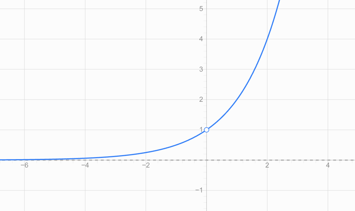
The graph has a distinctive curved shape. As x increases, the value of y increases more and more rapidly.
A few values help explain why:
| x | y = 2ˣ |
|---|---|
| -3 | 1/8 |
| -2 | 1/4 |
| -1 | 1/2 |
| 0 | 1 |
| 1 | 2 |
| 2 | 4 |
| 3 | 8 |
| 4 | 16 |
Notice that when x increases by 1, the value of y doubles.
This constant multiplication is one of the defining features of exponential functions.
Sketching an Exponential Graph
A useful way to sketch an exponential graph is to create a small table of values.
Consider:
y = 3ˣ
Choose several convenient x-values:
| x | y = 3ˣ |
|---|---|
| -2 | 1/9 |
| -1 | 1/3 |
| 0 | 1 |
| 1 | 3 |
| 2 | 9 |
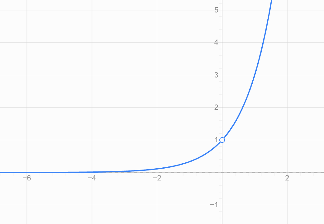
To sketch the graph:
- Choose several x-values on both sides of zero.
- Substitute each x-value into the function.
- Calculate the corresponding y-values.
- Plot the points.
- Connect them with a smooth curve.
- Examine what happens to the curve as x becomes very large or very negative.
Do not connect exponential points with straight line segments. An exponential graph is a smooth curve.
The Importance of x = 0
For a basic exponential function:
y = bˣ
something useful happens when x = 0.
Any non-zero number raised to the power zero equals 1:
b⁰ = 1
Therefore:
y = b⁰ = 1
This means every basic exponential function of the form y = bˣ passes through:
(0, 1)
For example:
- y = 2ˣ passes through (0, 1)
- y = 3ˣ passes through (0, 1)
- y = 5ˣ passes through (0, 1)
- y = (1/2)ˣ passes through (0, 1)
This is a very useful point when sketching.
Exponential Growth
An exponential function shows exponential growth when its values increase as x increases.
For:
y = a(bˣ)
growth occurs when:
b > 1
Examples include:
- y = 2ˣ
- y = 3ˣ
- y = 1.5ˣ
- y = 10ˣ
Compare several growth functions:
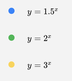
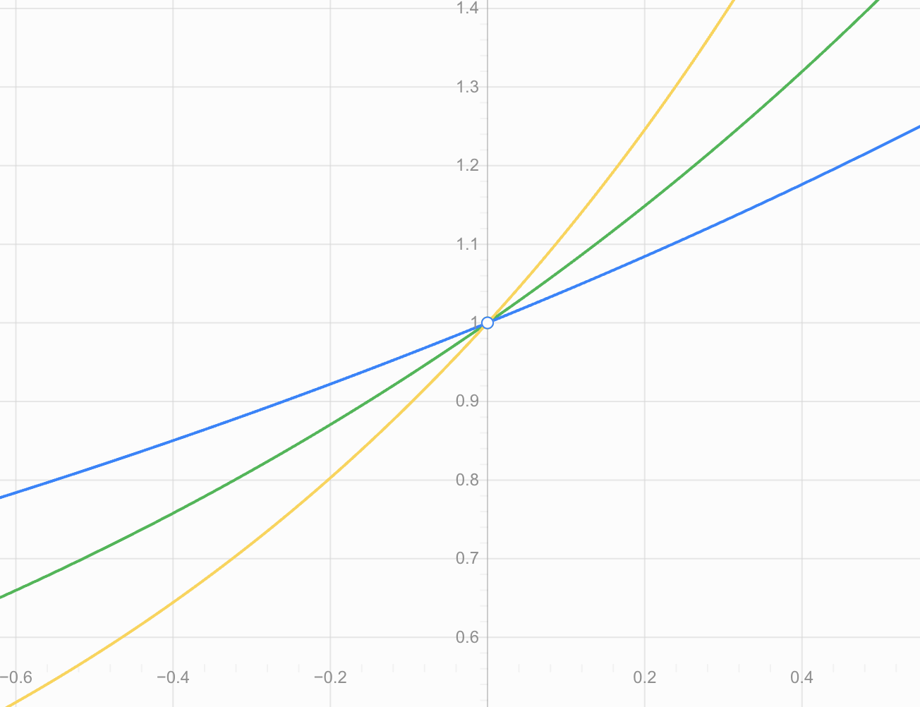
All three increase, but they do not increase at the same rate.
A larger growth factor generally produces faster growth.
For example, beginning at x = 0:
y = 2ˣ
1 → 2 → 4 → 8 → 16
while:
y = 3ˣ
1 → 3 → 9 → 27 → 81
The second function grows much more rapidly.
Growth Means Multiplication
One of the most important ideas about exponential functions is that equal changes in x cause the output to be multiplied by the same factor.
Consider:
y = 5(2ˣ)
| x | y |
|---|---|
| 0 | 5 |
| 1 | 10 |
| 2 | 20 |
| 3 | 40 |
| 4 | 80 |
Each time x increases by 1:
y is multiplied by 2.
This differs from a linear function, where equal changes in x produce equal additions or subtractions.
For example:
Linear: 5, 10, 15, 20, 25 → add 5
Exponential: 5, 10, 20, 40, 80 → multiply by 2
Exponential Decay
Not all exponential functions increase.
An exponential function shows exponential decay when:
0 < b < 1
For example:
y = (1/2)ˣ
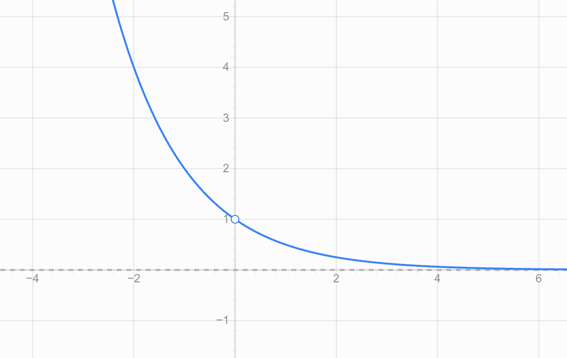
A table of values shows what is happening:
| x | y |
|---|---|
| -2 | 4 |
| -1 | 2 |
| 0 | 1 |
| 1 | 1/2 |
| 2 | 1/4 |
| 3 | 1/8 |
As x increases, y becomes smaller.
However, the values remain positive.
Decay Means Repeated Multiplication Too
Consider:
y = 100(0.5ˣ)
Starting at x = 0:
100 → 50 → 25 → 12.5 → 6.25
Each time x increases by 1, the previous value is multiplied by:
0.5
So exponential decay is not repeated subtraction.
The amount being lost becomes smaller each time because a constant proportion is being removed.
This is why exponential decay curves become flatter as they approach the x-axis.
Growth and Decay Compared
Compare:
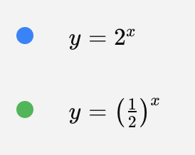
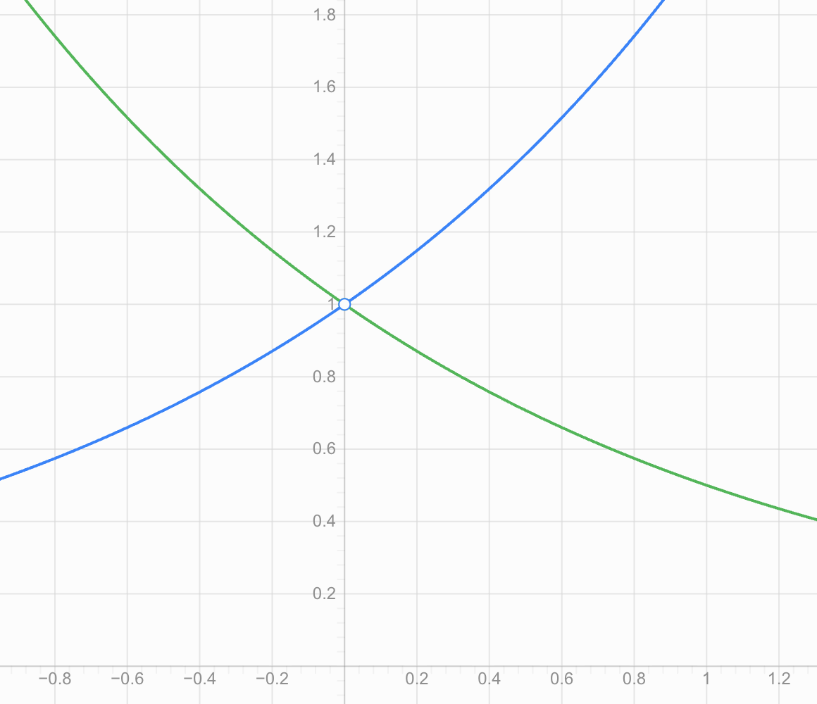
Both graphs:
- pass through (0, 1)
- remain above the x-axis
- have domain consisting of all real numbers
- have range y > 0
- approach y = 0
- never actually reach y = 0
But their directions are different.
Exponential growth: rises from left to right.
Exponential decay: falls from left to right.
Domain of an Exponential Function
The domain is the set of possible x-values.
For a basic exponential function such as:
y = 2ˣ
x can be:
- positive
- negative
- zero
- a fraction
- a decimal
For example:
2⁻³, 2⁰, 2¹·⁵ and 2⁴ are all defined.
Therefore, the domain is:
all real numbers
or:
−∞ < x < ∞
In interval notation:
(−∞, ∞)
This is true for basic exponential functions and their usual transformations.
Range of a Basic Exponential Function
The range is the set of possible y-values.
Consider again:
y = 2ˣ
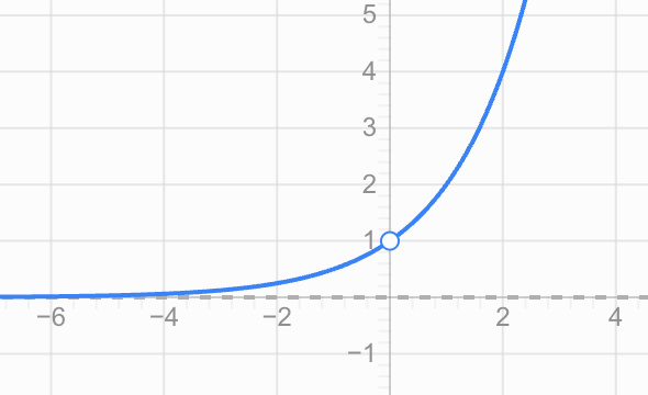
The output is always positive.
It can become extremely small:
0.1
0.01
0.001
and so on.
But it never becomes exactly zero.
It also never becomes negative.
Therefore, for y = 2ˣ:
Range: y > 0
or in interval notation:
(0, ∞)
Horizontal Asymptotes
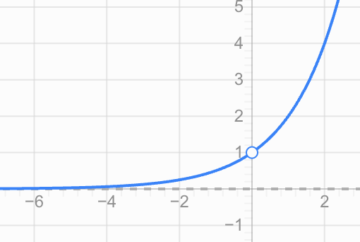
Look carefully at what happens to:
y = 2ˣ
as x becomes increasingly negative.
For example:
2⁻¹ = 0.5
2⁻² = 0.25
2⁻³ = 0.125
2⁻⁴ = 0.0625
2⁻⁵ = 0.03125
The values get closer and closer to zero.
However, 2ˣ never actually equals zero.
The line:
y = 0
is therefore a horizontal asymptote.
A horizontal asymptote is a horizontal line that a graph approaches as x moves far in one direction.
For a basic exponential function:
y = a(bˣ)
the horizontal asymptote is usually:
y = 0
Does an Exponential Graph Touch Its Asymptote?
For a basic positive exponential function, no.
For example:
y = 3ˣ
can become extremely close to zero, but:
3ˣ > 0
for every real value of x.
Therefore, its graph never reaches the x-axis.
This is why the x-axis acts as the horizontal asymptote.
An asymptote describes the long-term behaviour of the graph.
Shifting an Exponential Graph Vertically
Now consider:
y = 2ˣ + 3
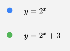
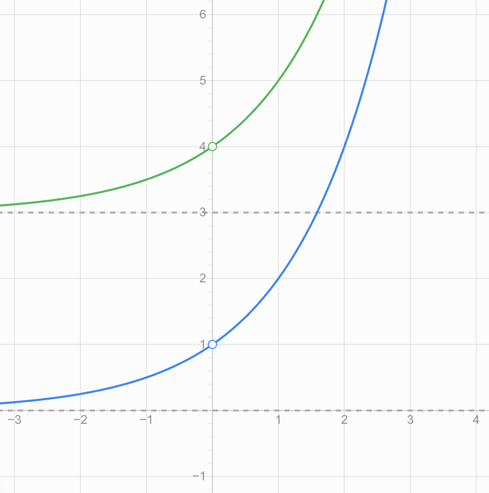
Adding 3 moves the entire graph 3 units upward.
The original function:
y = 2ˣ
has horizontal asymptote:
y = 0
The transformed function:
y = 2ˣ + 3
has horizontal asymptote:
y = 3
Its range also changes.
Instead of:
y > 0
the range becomes:
y > 3
A Useful General Form
A transformed exponential function can be written as:
y = a(bˣ) + k
The value k moves the graph vertically.
Its horizontal asymptote becomes:
y = k
For example:
y = 4(2ˣ) + 5
has horizontal asymptote:
y = 5
and, because the graph is above the asymptote:
Range: y > 5
A Reflection of an Exponential Graph
A negative coefficient can reflect an exponential graph across the x-axis.
Compare:
y = 2ˣ
and:
y = −2ˣ
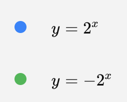
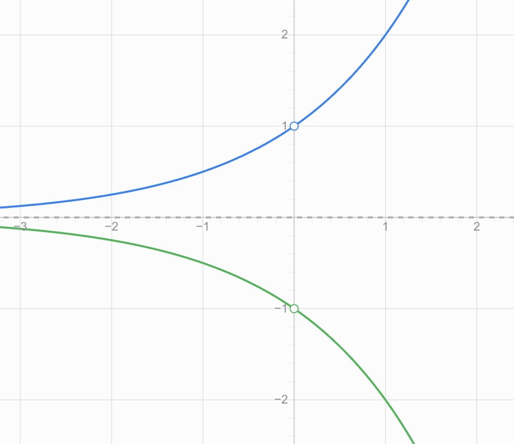
For y = −2ˣ:
- all outputs are negative
- the horizontal asymptote is still y = 0
- the domain is all real numbers
- the range is y < 0
This reminds us that the range is not always y > 0. We must examine the complete function.
Worked Example 1: Sketching an Exponential Growth Function
Sketch:
y = 2(3ˣ)
Step 1: Identify the base
The base is:
b = 3
Since:
3 > 1
the function represents exponential growth.
Step 2: Find some points
| x | y = 2(3ˣ) |
|---|---|
| -2 | 2/9 |
| -1 | 2/3 |
| 0 | 2 |
| 1 | 6 |
| 2 | 18 |
Step 3: Identify the asymptote
There is no vertical shift, so:
Horizontal asymptote: y = 0
Step 4: State the domain and range
Domain: all real numbers
Range: y > 0
Step 5: Sketch the curve
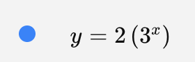
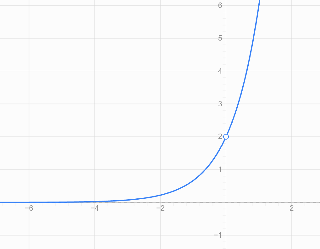
The graph rises increasingly rapidly from left to right.
Worked Example 2: Exponential Decay
Consider:
y = 8(0.5ˣ)
Because:
0 < 0.5 < 1
the function represents exponential decay.
Calculate some values:
| x | y |
|---|---|
| 0 | 8 |
| 1 | 4 |
| 2 | 2 |
| 3 | 1 |
| 4 | 0.5 |
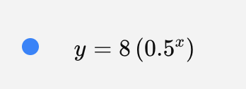
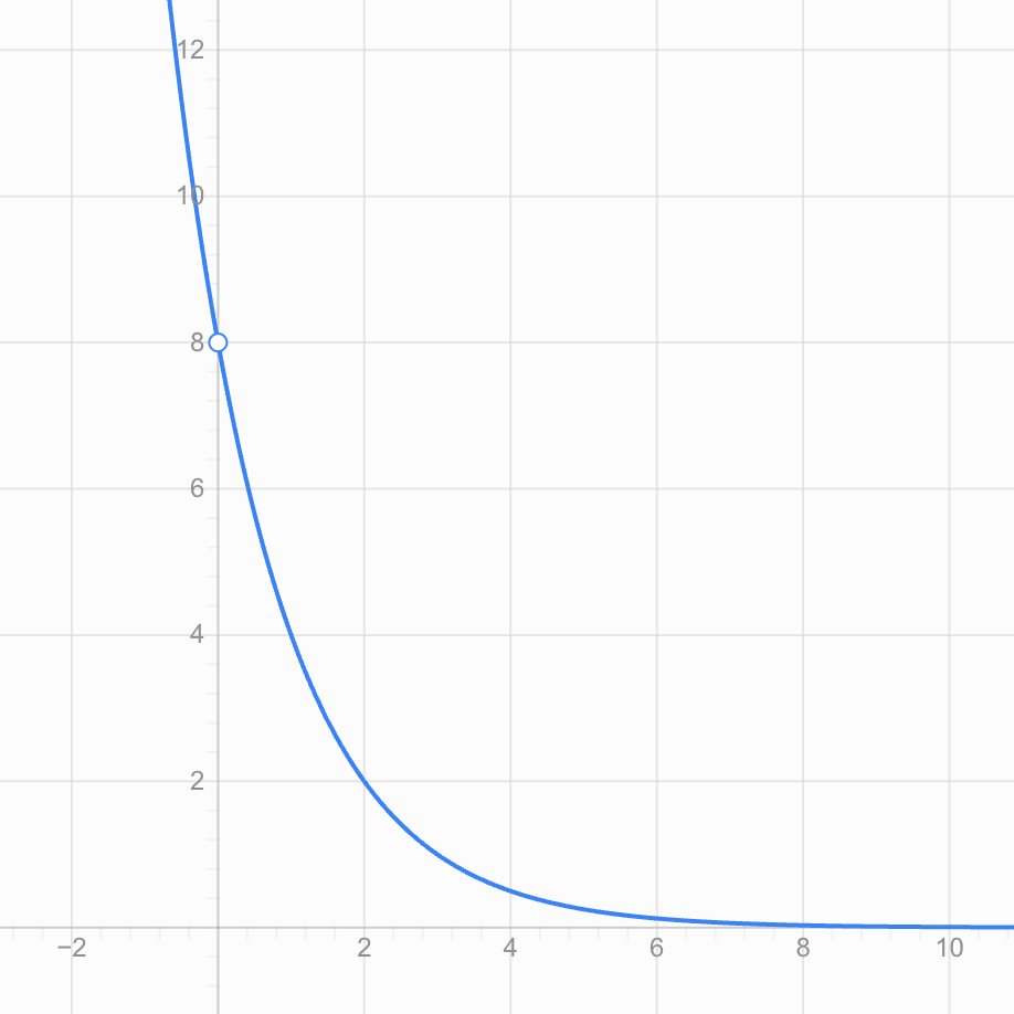
From the graph:
Domain: all real numbers
Range: y > 0
Horizontal asymptote: y = 0
Behaviour: y decreases toward zero as x increases.
Worked Example 3: Finding a Shifted Asymptote
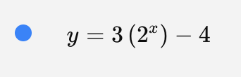
Consider:
y = 3(2ˣ) − 4
The −4 shifts the basic exponential graph downward by 4 units.
Therefore:
Horizontal asymptote: y = −4
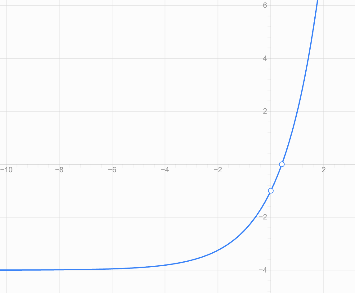
Because 3(2ˣ) is always positive, the graph remains above −4.
Therefore:
Domain: all real numbers
Range: y > −4
Interpreting Exponential Graphs in Context
Exponential functions are useful because many real-world quantities change by a constant percentage or constant multiplication factor.
Examples include:
- population growth
- bacterial growth
- compound interest
- radioactive decay
- depreciation
- cooling models
- spread of information
- some biological growth processes
The graph can tell us much more than whether a quantity is increasing or decreasing.
Example: Bacterial Growth
Suppose a bacterial population is modelled by:
P = 200(2ᵗ)
where:
- P is the bacterial population
- t is time in hours
At t = 0:
P = 200(2⁰)
P = 200
So the initial population is 200 bacteria.
After 1 hour:
P = 200(2¹) = 400
After 2 hours:
P = 200(2²) = 800
After 3 hours:
P = 200(2³) = 1600
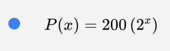
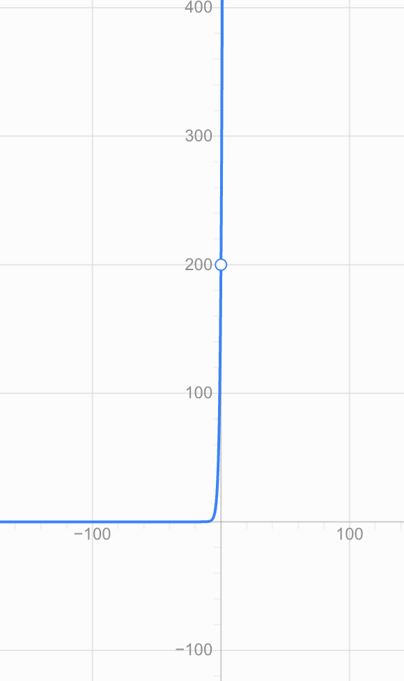
The graph becomes increasingly steep because the population doubles during every equal time interval.
In the real-world context, we would normally restrict the domain to:
t ≥ 0
because negative time may not make sense for the situation being modelled.
Example: Depreciation
Suppose a piece of equipment is initially worth $10,000 and retains 80% of its value each year.
Its value could be modelled by:
V = 10,000(0.8ᵗ)
Because:
0 < 0.8 < 1
this represents exponential decay.
After 1 year:
V = 10,000(0.8)
V = $8,000
After 2 years:
V = 10,000(0.8²)
V = $6,400
After 3 years:
V = 10,000(0.8³)
V = $5,120
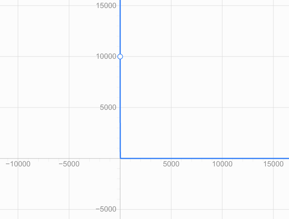
The graph approaches zero but does not reach zero according to the mathematical model.
In reality, an object might eventually have a minimum resale or scrap value, so mathematical models do not always describe reality perfectly forever.
Reading an Exponential Graph
When interpreting an exponential graph, ask several questions.
1. What does the horizontal axis represent?
It might represent:
- time
- distance
- number of periods
- age
2. What does the vertical axis represent?
It might represent:
- population
- money
- mass
- concentration
- temperature difference
3. What is the initial value?
Often this is the value when:
x = 0
4. Is the quantity growing or decaying?
Look at whether the graph rises or falls from left to right.
5. What value does the graph approach?
This can often be identified from the horizontal asymptote.
6. What restrictions make sense?
A mathematical function might allow all real x-values, but the real-world situation may not.
Linear Growth vs Exponential Growth
These two types of growth are easily confused.
Consider:
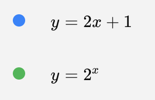
Linear: y = 2x + 1
Exponential: y = 2ˣ
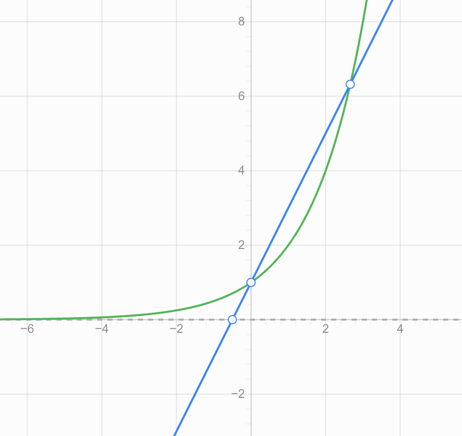
A linear function changes by a constant amount.
An exponential function changes by a constant factor or percentage.
For example:
| x | Linear: 2x + 1 | Exponential: 2ˣ |
|---|---|---|
| 0 | 1 | 1 |
| 1 | 3 | 2 |
| 2 | 5 | 4 |
| 3 | 7 | 8 |
| 4 | 9 | 16 |
| 5 | 11 | 32 |
The exponential function eventually grows much faster.
Common Mistakes
Mistake 1: Thinking exponential growth means constant addition
The sequence:
2, 4, 6, 8, 10
is not exponential.
It increases by 2 each time, so it shows a linear pattern.
The sequence:
2, 4, 8, 16, 32
is exponential because each term is multiplied by 2.
Mistake 2: Thinking an exponential graph eventually reaches its asymptote
For:
y = 2ˣ
the graph approaches y = 0 but never reaches it.
The x-axis is a horizontal asymptote.
Mistake 3: Assuming all exponential graphs increase
Functions with:
b > 1
show exponential growth.
Functions with:
0 < b < 1
show exponential decay.
Mistake 4: Saying the range is always y > 0
That is true for basic positive exponential functions such as:
y = 2ˣ
But transformations can change the range.
For:
y = 2ˣ + 5
the range is:
y > 5
Mistake 5: Confusing x² with 2ˣ
These functions are fundamentally different.
x² → quadratic
2ˣ → exponential
The position of the variable matters.
Key Terms
Exponential function — A function in which the variable occurs in the exponent.
Base — The number being raised to a power.
Exponential growth — An exponential pattern in which values increase by a constant multiplication factor.
Exponential decay — An exponential pattern in which values decrease by a constant multiplication factor between 0 and 1.
Domain — The set of possible input values.
Range — The set of possible output values.
Horizontal asymptote — A horizontal line that a graph approaches as x moves far in one direction.
Initial value — The output at the beginning of a model, commonly when x = 0.
Growth factor — The factor greater than 1 by which a quantity is repeatedly multiplied.
Decay factor — A factor between 0 and 1 by which a quantity is repeatedly multiplied.
Check Your Understanding
-
Is y = 4ˣ an exponential growth or decay function?
-
Is y = (0.3)ˣ growth or decay?
-
What point must the graph of y = 7ˣ pass through?
-
State the domain of y = 5ˣ.
-
State the range of y = 5ˣ.
-
What is the horizontal asymptote of y = 5ˣ?
-
What is the horizontal asymptote of y = 5ˣ + 4?
-
State the range of y = 5ˣ + 4.
-
Create a table of values for y = 2ˣ using x = −2, −1, 0, 1, 2 and sketch the graph.
-
A population is modelled by P = 500(1.2ᵗ). Is the population growing or decaying? Explain how you know.
-
A machine's value is modelled by V = 20,000(0.9ᵗ). What does 20,000 represent? What does 0.9 tell you about the machine's value?
-
Explain why an exponential decay graph can approach zero indefinitely without actually reaching zero.
Key Takeaways
- An exponential function has the variable in the exponent.
- A basic exponential function can be written as y = a(bˣ).
- If b > 1, the function shows exponential growth.
- If 0 < b < 1, the function shows exponential decay.
- Basic exponential functions have a domain of all real numbers.
- A basic positive exponential function has the range y > 0.
- The basic exponential graph has the horizontal asymptote y = 0.
- In y = a(bˣ) + k, the horizontal asymptote is y = k.
- Exponential change involves repeated multiplication, not repeated addition.
- Graphs should always be interpreted using the meaning of their axes and the context of the situation.
Did You Know?
Exponential growth can become surprisingly large very quickly. If a quantity doubles repeatedly, after only 10 doublings it is 1,024 times its original size. After 20 doublings, it is more than one million times its original size. This rapid change is one reason exponential models are so important in areas such as finance, biology, computing, and population studies.