Sampling Distributions

Introduction

When statisticians want to learn about a large population, it is often impractical to measure every individual.

For example, a researcher might want to determine the average height of all students in a country. Measuring every student would require considerable time and resources.

Instead, the researcher can select a smaller group, called a sample, and use its results to estimate characteristics of the entire population.

However, different samples will usually produce slightly different results.

One sample might have an average height of 165 cm, while another might have an average of 168 cm.

This natural variation leads to an important statistical concept: the sampling distribution.

A sampling distribution describes how a statistic, such as a sample mean or sample proportion, varies across repeated samples from the same population.

Sampling distributions are essential for understanding statistical uncertainty, confidence intervals, hypothesis testing, and the reliability of research findings.

Populations and Samples

Before studying sampling distributions, we need to distinguish between a population and a sample.

Population

A population is the complete group of individuals, objects, or observations that a researcher wants to investigate.

Examples include:

• All students attending a school.

• All households in a city.

• Every product manufactured during a month.

• All trees in a particular forest.

• Every voter in a country.

Sample

A sample is a subset of the population selected for investigation.

For example, a school may have 1,200 students, but a researcher might collect data from only 100 of them.

The 1,200 students form the population.

The 100 selected students form the sample.

Why Use Samples?

Sampling allows researchers to:

• Collect information more efficiently.

• Reduce the cost of investigations.

• Study populations that are too large to measure completely.

• Estimate unknown population characteristics.

• Make decisions using available evidence.

However, sample results are subject to uncertainty because different samples may contain different observations.

Population Parameters and Sample Statistics

A parameter is a numerical characteristic of a population.

A statistic is a numerical characteristic calculated from a sample.

Example

Suppose the true average height of all students in a school is 165 cm.

This is the population mean:

μ = 165 cm

A random sample of 40 students has an average height of 167 cm.

This is the sample mean:

x̄ = 167 cm

The sample mean differs from the population mean by 2 cm.

This difference is an example of sampling error.

Important Distinction

A population parameter is usually treated as a fixed, although potentially unknown, value.

A sample statistic can vary because it depends on which observations are selected.

What Is a Sampling Distribution?

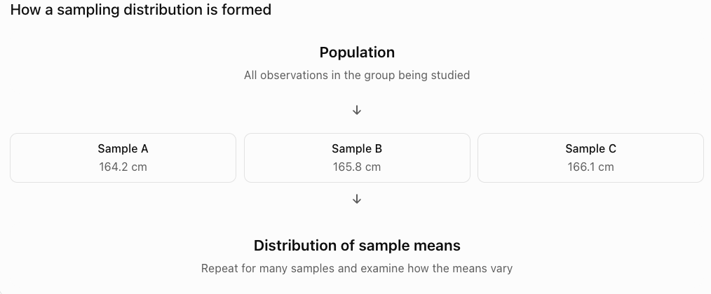
A sampling distribution is the probability distribution of a statistic calculated from all possible samples of a specified size under a particular sampling procedure.

For example, imagine repeatedly selecting random samples of 30 students from a school.

For each sample, calculate the mean height.

The results might be:

These values are sample means, not individual student heights.

If we repeatedly select samples and record their means, we can construct a distribution of sample means.

That distribution approximates the sampling distribution of the sample mean.

Important Observation

A sampling distribution describes the variation of a statistic, not the variation of individual observations.

This distinction is fundamental to statistical inference.

Three Different Distributions

It is important to distinguish between three related distributions.

Population Distribution

The distribution of all individual observations in the population.

For example, the heights of every student in a school.

Sample Distribution

The distribution of individual observations within one selected sample.

For example, the heights of 30 randomly selected students.

Sampling Distribution

The distribution of a statistic calculated from many possible samples of the same size.

For example, the means of thousands of random samples, each containing 30 students.

Example

Suppose a population has:

Mean = 100

Standard deviation = 20

One sample of 25 observations might have:

Sample mean = 104

Another sample might have:

Sample mean = 97

A third sample might have:

Sample mean = 101

The sampling distribution describes the probabilities associated with these possible sample means.

Sampling Variability

Sampling variability is the natural variation in sample statistics caused by selecting different samples from the same population.

Even when the population does not change, different random samples usually produce different results.

Example

Suppose a school has a population mean mathematics score of 70.

Five random samples of 20 students produce the following means:

68, 72, 69, 71, 70

The sample means vary slightly.

This variation is expected.

Why Does Sampling Variability Occur?

Different samples contain different individuals.

Some samples may include more high-scoring students.

Others may include more low-scoring students.

Consequently, the sample means differ.

Important Observation

Sampling variability does not necessarily indicate a mistake.

It is a normal feature of random sampling.

The Standard Error

The standard error measures the standard deviation of a sampling distribution.

For the sample mean, when observations are independent and drawn from a population with standard deviation σ:

SE(x̄) = σ/√n

where:

• SE(x̄) = standard error of the sample mean

• σ = population standard deviation

• n = sample size

Interpretation

The standard error describes how much sample means typically vary around the population mean.

A smaller standard error means that sample means are more tightly concentrated around the population mean.

A larger standard error means greater sampling variability.

Calculating Standard Error

Suppose a population has:

Mean = 80

Standard deviation = 12

A researcher selects independent random samples of size 36.

Calculate the standard error.

Step 1: Identify the Values

σ = 12

n = 36

Step 2: Apply the Formula

SE(x̄) = 12/√36

SE(x̄) = 12/6

SE(x̄) = 2

Interpretation

The standard deviation of the sampling distribution of sample means is 2.

Although individual observations have a standard deviation of 12, the sample means vary much less.

How Sample Size Affects Sampling Variability

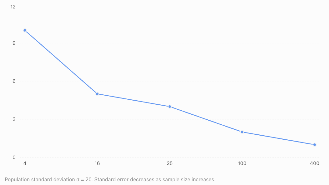
One of the most important properties of sampling distributions is that larger samples generally produce more precise estimates.

For the sample mean:

SE(x̄) = σ/√n

As n increases, the denominator increases.

Therefore, the standard error decreases.

Example

Suppose:

σ = 20

Compare the standard errors for different sample sizes.

Important Conclusion

Larger samples tend to produce more stable sample means.

However, the improvement follows a square-root relationship.

To reduce the standard error by half, the sample size must be multiplied by four.

Example

If a sample of 25 has a standard error of 4, a sample of 100 will have a standard error of 2, assuming the same population and sampling conditions.

Standard Deviation Versus Standard Error

Standard deviation and standard error measure different types of variability.

Example

A population of students has:

Mean height = 165 cm

Standard deviation = 10 cm

A sample of 100 students is selected.

Standard error:

SE = 10/√100

SE = 1 cm

Interpretation

The standard deviation of 10 cm describes differences among individual student heights.

The standard error of 1 cm describes the spread of sample means from repeated samples of 100 students.

These are not interchangeable quantities.

The Central Limit Theorem

The Central Limit Theorem (CLT) is one of the most important ideas in statistics.

It explains why normal distributions frequently appear when analysing sample means.

Statement of the Central Limit Theorem

For independent, identically distributed observations from a population with a finite mean and finite variance, the sampling distribution of the sample mean becomes approximately normal as the sample size increases.

This can occur even when the original population is not normally distributed.

Important Features

• The original population does not need to be normal.

• The sample size must be sufficiently large.

• The population must have a finite mean and variance under the classical version of the theorem.

• The sampling distribution becomes approximately normal as n increases.

• The sampling distribution is centred at the population mean.

• Its standard error is σ/√n for independent observations.

Understanding the Central Limit Theorem

Consider a population with a strongly right-skewed distribution.

Individual observations may be concentrated near low values, with a long tail toward high values.

Now imagine repeatedly selecting random samples and calculating their means.

Small Samples

When the sample size is very small, the distribution of sample means may still be noticeably skewed.

Larger Samples

As the sample size increases, the sampling distribution of the mean generally becomes more symmetric.

Very Large Samples

For sufficiently large samples, the sampling distribution often resembles a normal distribution.

This happens because averaging many independent observations reduces the influence of individual extreme values.

Important Qualification

There is no universal sample size that guarantees a good normal approximation.

The required sample size depends on the shape of the population distribution.

A commonly taught guideline is n ≥ 30, but strongly skewed or heavy-tailed populations may require much larger samples.

When the Population Is Already Normal

If the population itself is normally distributed, the sampling distribution of the sample mean is normal for every positive sample size, assuming independent observations.

Suppose:

X ~ N(μ, σ²)

Then:

x̄ ~ N(μ, σ²/n)

Example

A population has:

Mean = 50

Standard deviation = 10

Independent random samples of size 25 are selected.

The sampling distribution of the sample mean has:

Mean = 50

Standard error = 10/√25 = 2

Therefore:

x̄ ~ N(50, 4)

The second parameter is the variance of the sampling distribution.

Mean of the Sampling Distribution

The mean of the sampling distribution of the sample mean is equal to the population mean.

E(x̄) = μ

This means the sample mean is an unbiased estimator of the population mean under random sampling.

Example

Suppose the population mean is 75.

If we repeatedly select independent random samples and calculate their means, the average of those sample means approaches 75.

Individual samples may produce means above or below 75.

However, the sampling distribution is centred at 75.

Important Observation

Unbiased does not mean every sample estimate is correct.

It means the estimator is correct on average across repeated samples.

Calculating Probabilities Using Sampling Distributions

When the sampling distribution of the mean is normal or approximately normal, we can calculate probabilities using z-scores.

The z-score formula for a sample mean is:

z = (x̄ − μ)/(σ/√n)

This differs from the z-score formula for an individual observation.

For an individual observation:

z = (x − μ)/σ

For a sample mean:

z = (x̄ − μ)/(σ/√n)

The denominator is the standard error rather than the population standard deviation.

Worked Example: Sample Mean Above a Value

A population has:

Mean = 100

Standard deviation = 20

Independent random samples of size 64 are selected.

Assume the sampling distribution is approximately normal.

Find the probability that a sample mean exceeds 105.

Step 1: Calculate the Standard Error

SE = 20/√64

SE = 20/8

SE = 2.5

Step 2: Calculate the z-Score

z = (105 − 100)/2.5

z = 5/2.5

z = 2

Step 3: Find the Probability

P(Z > 2) = 1 − 0.9772

P(Z > 2) ≈ 0.0228

Interpretation

There is approximately a 2.28% probability that a sample of 64 observations will have a mean greater than 105.

This probability describes sample means, not individual observations.

Worked Example: Sample Mean Below a Value

A population has:

Mean = 60

Standard deviation = 12

Independent random samples of size 36 are selected.

Assume the sampling distribution is approximately normal.

Find the probability that a sample mean is below 57.

Step 1: Calculate Standard Error

SE = 12/√36

SE = 2

Step 2: Calculate the z-Score

z = (57 − 60)/2

z = −1.5

Step 3: Find the Probability

P(Z < −1.5) = 0.0668

Final Answer

There is approximately a 6.68% probability that the sample mean is below 57.

Worked Example: Sample Mean Between Two Values

A population has:

Mean = 80

Standard deviation = 15

Independent random samples of size 100 are selected.

Assume the sampling distribution is approximately normal.

Find the probability that the sample mean lies between 77 and 83.

Step 1: Calculate Standard Error

SE = 15/√100

SE = 1.5

Step 2: Calculate the Lower z-Score

z₁ = (77 − 80)/1.5

z₁ = −2

Step 3: Calculate the Upper z-Score

z₂ = (83 − 80)/1.5

z₂ = 2

Step 4: Calculate the Probability

P(−2 ≤ Z ≤ 2) = 0.9772 − 0.0228

P(−2 ≤ Z ≤ 2) ≈ 0.9544

Interpretation

Approximately 95.44% of sample means are expected to fall between 77 and 83.

Sampling Distributions of Proportions

Sampling distributions are not limited to sample means.

They can also describe sample proportions.

Suppose a population contains a proportion p of individuals with a particular characteristic.

A sample is selected, and the proportion possessing that characteristic is calculated.

The sample proportion is represented by:

p̂

Example

Suppose 60% of students at a school prefer online homework.

The population proportion is:

p = 0.60

A random sample of 100 students might produce:

p̂ = 0.57

Another sample might produce:

p̂ = 0.63

These sample proportions vary because of sampling variability.

Mean and Standard Error of a Sample Proportion

Under independent Bernoulli sampling with constant success probability p:

E(p̂) = p

The standard error is:

SE(p̂) = √[p(1 − p)/n]

Worked Example

Suppose:

p = 0.60

n = 100

Calculate the standard error.

Step 1: Substitute

SE(p̂) = √[(0.60 × 0.40)/100]

SE(p̂) = √0.0024

SE(p̂) ≈ 0.049

Interpretation

The sample proportion typically varies around the population proportion by an amount on the order of 0.049, or 4.9 percentage points.

This does not mean every sample proportion will lie within 4.9 percentage points of the true proportion.

Normal Approximation for Sample Proportions

The sampling distribution of a sample proportion can often be approximated by a normal distribution when the sample size is sufficiently large.

A common guideline is:

np ≥ 10

and

n(1 − p) ≥ 10

Example

Suppose:

n = 100

p = 0.60

Then:

np = 60

n(1 − p) = 40

Both values exceed 10.

A normal approximation is generally reasonable under the independence assumptions.

Important Observation

Sample means and sample proportions have different standard-error formulas.

For sample means:

SE(x̄) = σ/√n

For sample proportions:

SE(p̂) = √[p(1 − p)/n]

Sampling With and Without Replacement

Sampling methods can affect the variability of sample statistics.

Sampling With Replacement

After an observation is selected, it is returned to the population before the next selection.

The same observation may be selected more than once.

Under simple random sampling with replacement, draws are independent.

Sampling Without Replacement

After an observation is selected, it is not returned.

The same individual cannot be selected again within that sample.

Draws are dependent because the population changes after each selection.

Why Does This Matter?

When sampling without replacement from a finite population, the standard error may be smaller than the independent-sampling formula suggests.

For a simple random sample without replacement from a finite population, the finite population correction is:

FPC = √[(N − n)/(N − 1)]

The corrected standard error of the sample mean is:

SE(x̄) = (σ/√n) × FPC

This correction is especially relevant when the sample represents a substantial fraction of the population.

For small sampling fractions, the correction is often negligible.

Sampling Error Versus Sampling Bias

Sampling error and sampling bias are different concepts.

Sampling Error

Sampling error is the difference between a sample statistic and the population parameter caused by random selection.

It occurs naturally even when the sampling method is fair.

Sampling Bias

Sampling bias occurs when the selection process systematically favours certain observations.

Example

A school wants to estimate how many students enjoy physical education.

If the researcher surveys only students participating in sports teams, the results may overestimate enthusiasm for physical education.

This is sampling bias.

Important Observation

Increasing sample size reduces random sampling variability.

However, increasing sample size does not automatically eliminate sampling bias.

A very large biased sample can still produce misleading conclusions.

Interpreting Sampling Distribution Graphs

Sampling distributions are commonly represented using histograms or probability curves.

Centre

The centre represents the expected value of the statistic.

For the sample mean:

E(x̄) = μ

Spread

The spread describes sampling variability.

For independent sample means:

SE(x̄) = σ/√n

Shape

The shape depends on the population distribution, sample size, and statistic being examined.

Larger Samples

Larger samples usually produce narrower sampling distributions.

This means the sample statistic is more likely to be close to the population parameter.

Important Interpretation

A narrower sampling distribution indicates greater precision.

It does not necessarily mean the individual observations are less variable.

Real-World Application: Opinion Polling

Opinion polls use samples to estimate the views of larger populations.

Example

A survey estimates that 55% of voters support a proposal.

The sample contains 400 independently selected respondents.

Using the sample proportion as an estimate of p:

p̂ = 0.55

n = 400

Estimated standard error:

SE ≈ √[(0.55 × 0.45)/400]

SE ≈ √0.00061875

SE ≈ 0.0249

Interpretation

The estimated standard error is approximately 2.49 percentage points.

This provides information about random sampling uncertainty.

Other sources of uncertainty, including nonresponse and selection bias, must also be considered.

Real-World Application: Manufacturing Quality Control

Manufacturers use sampling distributions to monitor production processes.

Example

A factory produces components with:

Mean mass = 250 g

Standard deviation = 8 g

A random sample of 64 independent components is selected.

Calculate Standard Error

SE = 8/√64

SE = 8/8

SE = 1 g

Interpretation

The sample mean mass typically varies around the population mean by an amount on the order of 1 g.

A sample mean far from 250 g may indicate an unusual sample or a possible change in the manufacturing process.

However, an unusual sample mean alone does not prove that the process has changed.

Real-World Application: Educational Research

Researchers may use sampling distributions to estimate average examination performance.

Example

A school has 2,000 students.

A researcher selects a random sample of 100 students to estimate average mathematics performance.

The sample mean is 72.

The sample standard deviation is 15.

An estimated standard error is:

SE ≈ 15/√100

SE ≈ 1.5

Interpretation

The estimated standard error describes the sampling variability of the sample mean.

It helps researchers judge the precision of the estimate.

Because the population standard deviation is unknown, the sample standard deviation is used as an estimate.

Real-World Application: Environmental Science

Environmental scientists often estimate population characteristics from samples.

Examples include:

• Average water temperature.

• Mean pollutant concentration.

• Average soil moisture.

• Proportion of contaminated samples.

• Average rainfall over a region.

Example

A researcher collects independent water samples from a large lake.

Each sample provides an estimate of the mean pollutant concentration.

Repeated sampling would produce slightly different sample means.

The sampling distribution describes this variation.

Important Consideration

Environmental observations may be correlated across locations or time.

If measurements are not independent, the usual standard-error formula may underestimate uncertainty.

Appropriate sampling designs are therefore important.

Common Mistakes

Confusing a population with a sample

The population is the complete group; the sample is a subset.

Confusing parameters with statistics

Parameters describe populations. Statistics describe samples.

Confusing the sample distribution with the sampling distribution

The sample distribution describes individual observations within one sample.

The sampling distribution describes a statistic across repeated samples.

Assuming every sample gives the same result

Different random samples generally produce different statistics.

Confusing standard deviation with standard error

Standard deviation measures variability among observations.

Standard error measures variability among sample statistics.

Using σ instead of σ/√n for sample-mean probabilities

The sampling distribution of the mean has a smaller spread than the population distribution under independent sampling.

Assuming larger samples eliminate all uncertainty

Larger samples reduce random sampling variability but do not eliminate it.

Assuming the Central Limit Theorem makes the population normal

The theorem concerns the sampling distribution of the mean, not the original population.

Assuming n = 30 always guarantees normality

The required sample size depends on the population distribution.

Ignoring independence assumptions

Dependent observations may require different methods.

Confusing sampling error with sampling bias

Sampling error arises from random variation; bias arises from systematic problems in selection or measurement.

Assuming an unbiased estimator is always accurate

Unbiased means correct on average, not correct in every sample.

Key Terms

• Population: Complete group of individuals or observations being studied.

• Sample: Subset of a population.

• Population Parameter: Numerical characteristic of a population.

• Sample Statistic: Numerical characteristic calculated from a sample.

• Population Mean (μ): Average of all population observations.

• Sample Mean (x̄): Average of observations within a sample.

• Population Standard Deviation (σ): Measure of population variability.

• Sample Standard Deviation (s): Measure of variability within a sample.

• Sampling Distribution: Probability distribution of a statistic across possible samples.

• Sampling Variability: Natural variation in sample statistics caused by random sampling.

• Sampling Error: Difference between a sample statistic and its population parameter.

• Standard Error: Standard deviation of a sampling distribution.

• Central Limit Theorem: Theorem describing the approximate normality of sample means for sufficiently large independent samples under suitable conditions.

• Unbiased Estimator: Estimator whose expected value equals the parameter being estimated.

• Sample Size : Number of observations in a sample.

• Population Size (N): Number of observations in the population.

• Random Sampling: Sampling process involving random selection.

• Sampling With Replacement: Method in which selected observations are returned before subsequent selections.

• Sampling Without Replacement: Method in which selected observations are not returned.

• Finite Population Correction: Adjustment for sampling without replacement from a finite population.

• Sample Proportion (p̂): Proportion of sample observations with a particular characteristic.

• Population Proportion (p): Proportion of the population with a particular characteristic.

• Normal Approximation: Use of a normal distribution to approximate another distribution.

• Sampling Bias: Systematic distortion caused by the sampling process.

• Statistical Inference: Use of sample information to draw conclusions about populations.

• Precision: Degree to which repeated estimates are concentrated around one another.

Key Takeaways

• Sampling distributions describe how sample statistics vary across repeated samples.

• A population parameter is fixed, while a sample statistic varies from sample to sample.

• Sampling variability occurs naturally because different samples contain different observations.

• The sampling distribution of the sample mean is centred at the population mean.

• The standard error measures the spread of the sampling distribution.

• For independent observations, SE(x̄) = σ/√n.

• Larger samples generally produce smaller standard errors.

• To halve the standard error, the sample size must be multiplied by four.

• The Central Limit Theorem explains why sample means often follow approximately normal distributions for sufficiently large samples.

• The original population does not need to be normally distributed.

• A normal population produces normally distributed sample means for any sample size under independent sampling.

• Sample means and sample proportions have different standard-error formulas.

• Sampling error is different from sampling bias.

• Larger samples reduce random sampling variability but do not automatically correct biased sampling.

• Sampling distributions are fundamental to statistical inference, confidence intervals, and hypothesis testing.

Check Your Understanding

Populations and Samples

1. Define a population.

2. Define a sample.

3. Explain the difference between a parameter and a statistic.

4. What symbol represents the population mean?

5. What symbol represents the sample mean?

Sampling Distributions

6. Define a sampling distribution.

7. Explain why sample means vary between samples.

8. What is sampling variability?

9. What is the mean of the sampling distribution of the sample mean?

10. Explain the difference between standard deviation and standard error.

Central Limit Theorem

11. State the Central Limit Theorem in your own words.

12. Does the original population need to be normal?

13. What generally happens to the sampling distribution as sample size increases?

14. Why is n = 30 not a universal guarantee of normality?

15. Explain why the Central Limit Theorem is important in statistics.

Calculations

16. Calculate the standard error when σ = 20 and n = 25.

17. Calculate the standard error when σ = 15 and n = 100.

18. A population has mean 80, standard deviation 12, and sample size 36. Calculate the z-score for a sample mean of 84.

19. A population proportion is 0.40 and n = 100. Calculate the standard error of the sample proportion.

20. Explain what happens to standard error when sample size is multiplied by four.

Answer Key

Extended Challenge

Understanding Sampling Distributions

1. Explain why the sampling distribution of the mean is different from the population distribution.

2. Describe how repeated random sampling can be used to construct a sampling distribution.

3. Explain why the sample mean is an unbiased estimator of the population mean.

4. Describe the effect of increasing sample size on sampling variability.

5. Explain why a larger sample does not necessarily eliminate sampling bias.

Standard Error Calculations

6. Calculate the standard error for σ = 24 and n = 36.

7. Calculate the standard error for σ = 18 and n = 81.

8. Calculate the sample size required to reduce a standard error of 6 to 3.

9. A population has standard deviation 30. Find the sample size required for a standard error of 3.

10. Explain why standard error decreases according to a square-root relationship.

Central Limit Theorem

11. Explain why sample means can be approximately normal even when the population is skewed.

12. Describe a situation where the Central Limit Theorem might require a very large sample.

13. Explain why the sampling distribution of a normal population is normal for every sample size.

14. Discuss the importance of independence in the Central Limit Theorem.

15. Explain why the theorem is useful for calculating probabilities.

Practical Applications

16. A population has mean 100 and standard deviation 20. Independent samples of size 100 are selected. Find P(x̄ > 104), assuming an approximately normal sampling distribution.

17. A population has mean 60 and standard deviation 15. Independent samples of size 25 are selected. Find P(x̄ < 57), assuming an approximately normal sampling distribution.

18. A population proportion is 0.30. Find the standard error for n = 400 under independent Bernoulli sampling.

19. Explain how sampling distributions help researchers estimate population characteristics.

20. Describe how sampling bias can affect conclusions even when the standard error is small.

Final Investigation: Estimating Student Examination Performance

A school has 2,500 students.

The population mean mathematics score is 70.

The population standard deviation is 15.

Researchers investigate the sampling distribution of the mean using independent random samples.

Investigation Tasks

1. Identify the population.

2. Identify the population mean.

3. Identify the population standard deviation.

4. Explain what a sample mean represents.

5. Define the sampling distribution of the sample mean.

6. Calculate the standard error for n = 25.

7. Calculate the standard error for n = 100.

8. Calculate the standard error for n = 225.

9. Compare the three standard errors.

10. Explain why larger samples produce smaller standard errors.

11. Sketch the sampling distributions for the three sample sizes on the same scale.

12. Identify which distribution is narrowest.

13. Explain why all three distributions have the same centre.

14. Calculate the z-score for x̄ = 73 when n = 100.

15. Find P(x̄ > 73) for n = 100, assuming an approximately normal sampling distribution.

16. Calculate the probability that x̄ lies between 67 and 73 when n = 100.

17. Explain how the Central Limit Theorem supports the probability calculations.

18. Discuss why a biased sample might produce misleading results.

19. Explain how the researchers could improve the sampling procedure.

20. Write a statistical report describing the relationship between sample size, standard error, and the reliability of sample estimates.