Normal Distribution

Introduction

Many measurements in the real world tend to cluster around an average value, with fewer observations occurring far above or below that average.

For example, when measuring the heights of a large group of people of similar age, most measurements may be near the average height. Very short and very tall measurements are generally less common.

This pattern can often be described using the normal distribution.

The normal distribution is one of the most important probability distributions in mathematics and statistics. It is widely used in scientific research, education, manufacturing, medicine, economics, and quality control.

It allows us to calculate the probability of a measurement falling within a particular range, determine how unusual an observation is, and compare results from different datasets.

 

 

 

 

 

 

wQI6-jisIRlogp3oymKZba5mnc9mXGz426qzidVhdFh8AoCnsn60YpqhbjarVIGv7XJ31I0VDKHkGZVTHx7MQX_6HuRMYXhVEz1MV2IZO4nyLW1YVDUUv_ER3huob9-2D4XDusoXD9SupJEHAarcur2UG8Ow8Y?purpose=inline" alt="Quality Control Training Certificate | Free & Fast Course">

 

9

 

What Is a Normal Distribution?

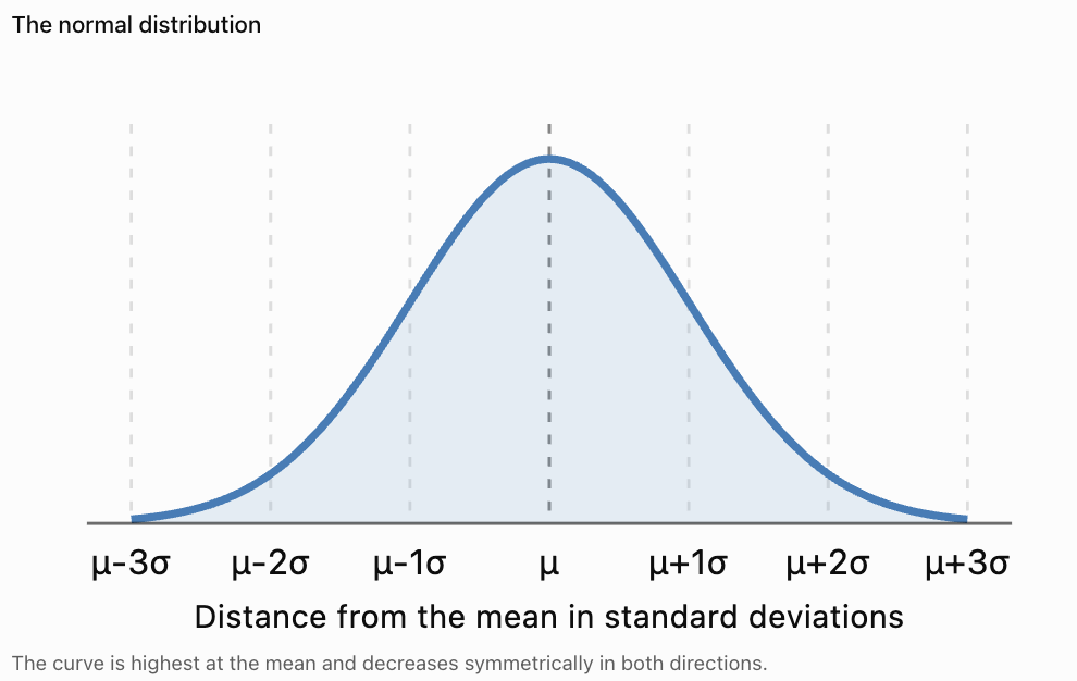
A normal distribution is a continuous probability distribution that is symmetric about its mean and has a characteristic bell-shaped curve.

The highest point of the curve occurs at the mean.

As values move farther from the mean, the probability density decreases.

Characteristics of the Normal Distribution

• The distribution is symmetric about its mean.

• It has one peak, making it unimodal.

• The mean, median, and mode are equal.

• The total area under the curve is 1.

• The curve extends indefinitely in both directions.

• The tails approach, but never touch, the horizontal axis.

• Its shape is determined by the mean and standard deviation.

  

  Important Observation

  Not every bell-shaped dataset follows a perfectly normal distribution.

  The normal distribution is a mathematical model. Real data may only approximate this shape.

   

  The Mean and Standard Deviation

  Two values completely determine a normal distribution.

  Mean (μ)

  The mean determines the centre of the distribution.

  If the mean changes, the entire curve shifts left or right.

  Standard Deviation (σ)

  The standard deviation determines the spread of the distribution.

  A smaller standard deviation produces a narrower, taller curve.

  A larger standard deviation produces a wider, flatter curve.

  

   

   

   

  metricgate.com

  Example

  Consider two normally distributed examination results.

  Statistic	Class A	Class B
  Mean	70	70
  Standard deviation	5	15

  Both classes have the same average score.

  However, Class A has less variation.

  Most students in Class A score relatively close to 70.

  Class B has a much wider spread of results.

  Interpretation

  The mean describes the centre.

  The standard deviation describes the variability.

  Both are needed to understand a normal distribution.

   

  Notation for the Normal Distribution

  A normal random variable is commonly written as:

  X ~ N(μ, σ²)

  where:

  • X = random variable

  • μ = population mean

  • σ² = population variance

  • σ = population standard deviation

  Example

  Suppose examination scores are normally distributed with:

  Mean = 70

  Standard deviation = 10

  The variance is:

  σ² = 10² = 100

  Therefore:

  X ~ N(70, 100)

  Important Distinction

  In this notation, the second parameter is the variance, not the standard deviation.

  Some calculators ask for the mean and standard deviation separately, so always check the required inputs.

   

  Understanding Area Under the Curve

  The normal distribution is a continuous probability distribution.

  For a continuous random variable, probability is represented by area under the curve.

  The total area under the curve is:

  1 or 100%

  Example

  Suppose X represents the height of a randomly selected person from a population whose heights are approximately normally distributed.

  The probability that X lies between 160 cm and 180 cm is represented by the area under the curve between those two values.

  

   

   

   

  openstax.org

  Important Properties

  For any continuous random variable:

  P(X = a) = 0

  This means the probability of obtaining one exact mathematical value is zero.

  However, probabilities over intervals can be positive.

  For example:

  P(160 ≤ X ≤ 180)

  may be substantial.

  Why Does This Happen?

  A single point has no width and therefore no area.

  An interval has width, so the area under the curve can represent a nonzero probability.

   

  The Empirical Rule

  One of the most useful features of the normal distribution is the 68–95–99.7 rule.

  This rule describes approximately how much of the distribution lies within one, two, and three standard deviations of the mean.

  The empirical rule

  68%

  Within μ ± 1σ

  95%

  Within μ ± 2σ

  99.7%

  Within μ ± 3σ

  Within One Standard Deviation

  Approximately 68% of observations lie between:

  μ − σ and μ + σ

  Within Two Standard Deviations

  Approximately 95% of observations lie between:

  μ − 2σ and μ + 2σ

  Within Three Standard Deviations

  Approximately 99.7% of observations lie between:

  μ − 3σ and μ + 3σ

  Example

  Suppose examination scores have:

  Mean = 70

  Standard deviation = 10

  Approximately:

  • 68% of scores lie between 60 and 80.

  • 95% lie between 50 and 90.

  • 99.7% lie between 40 and 100.

  These percentages assume a normal model. If scores are restricted to 0–100, an exact normal distribution is not possible, although a normal approximation may still be useful.

   

  Understanding the Regions of a Normal Distribution

  Because the normal distribution is symmetric, we can divide the empirical-rule percentages between the left and right sides.

  Approximately:

  Region	Percentage
  Between μ and μ + σ	34%
  Between μ + σ and μ + 2σ	13.5%
  Between μ + 2σ and μ + 3σ	2.35%
  Beyond μ + 3σ	0.15%

  The same approximate percentages apply on the left side.

  Worked Example

  A normal distribution has mean 100 and standard deviation 15.

  Estimate the percentage of observations between 100 and 115.

  Since:

  115 = μ + σ

  The interval is from the mean to one standard deviation above the mean.

  Approximately half of 68% lies in this interval.

  Probability ≈ 34%

  Interpretation

  Approximately 34% of observations lie between 100 and 115.

   

  The Standard Normal Distribution

  The standard normal distribution is a special normal distribution with:

  Mean = 0

  Standard deviation = 1

  It is written:

  Z ~ N(0, 1)

  The horizontal axis is measured in standard scores called z-scores.

  

   

   

   

  biorender.com

  Why Is It Useful?

  Different normal distributions may have different means and standard deviations.

  By converting observations into z-scores, we can use one standard normal distribution to calculate probabilities for all of them.

  This process is called standardisation.

   

  Calculating z-Scores

  A z-score measures how many standard deviations an observation lies above or below the mean.

  The formula is:

  z = (x − μ)/σ

  where:

  • z = standard score

  • x = observed value

  • μ = population mean

  • σ = population standard deviation

  Interpretation

  • z = 0 means the observation equals the mean.

  • z = 1 means one standard deviation above the mean.

  • z = −1 means one standard deviation below the mean.

  • z = 2 means two standard deviations above the mean.

  • z = −2 means two standard deviations below the mean.

  Worked Example

  A normally distributed examination has:

  Mean = 65

  Standard deviation = 8

  A student scores 81.

  Calculate the z-score.

  Step 1: Identify the Values

  x = 81

  μ = 65

  σ = 8

  Step 2: Substitute

  z = (81 − 65)/8

  z = 16/8

  z = 2

  Interpretation

  The student scored two standard deviations above the mean.

  This is a relatively high result compared with the reference distribution.

   

  Calculating Negative z-Scores

  A negative z-score indicates an observation below the mean.

  Worked Example

  A normal distribution has:

  Mean = 50

  Standard deviation = 6

  An observation has value 41.

  Calculate:

  z = (41 − 50)/6

  z = −9/6

  z = −1.5

  Interpretation

  The observation is 1.5 standard deviations below the mean.

  The negative sign describes its position relative to the mean.

  It does not indicate that the original observation is negative.

   

  Using Standard Normal Tables

  A standard normal table provides probabilities associated with z-scores.

  Most common z-tables give the cumulative probability:

  P(Z ≤ z)

  This represents the area under the standard normal curve to the left of z.

  Common z-Scores and Probabilities

  z-score	P(Z ≤ z)
  −2.00	0.0228
  −1.50	0.0668
  −1.00	0.1587
  −0.50	0.3085
  0.00	0.5000
  0.50	0.6915
  1.00	0.8413
  1.50	0.9332
  2.00	0.9772
  2.50	0.9938
  3.00	0.9987

  Important Observation

  A z-table value is not the height of the curve.

  It represents an area, or cumulative probability.

   

  Calculating Probabilities Below a Value

  Suppose:

  X ~ N(70, 100)

  This means:

  Mean = 70

  Standard deviation = 10

  Find:

  P(X < 85)

  Step 1: Convert to a z-Score

  z = (85 − 70)/10

  z = 1.5

  Step 2: Use the Standard Normal Table

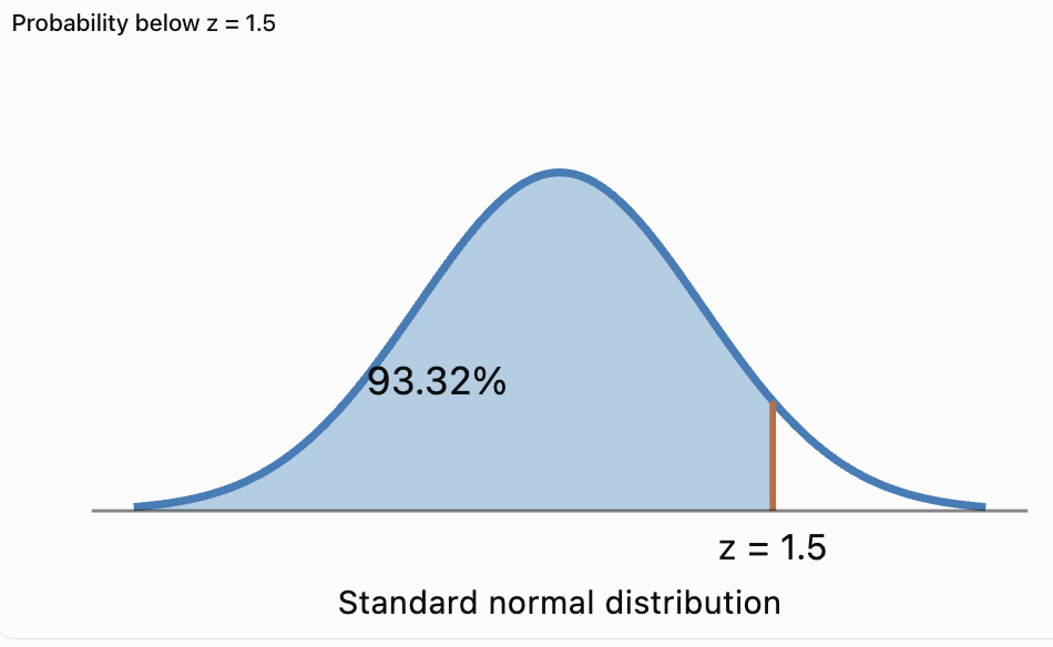
  P(Z < 1.5) = 0.9332

  Final Answer

  P(X < 85) ≈ 0.9332

  There is approximately a 93.32% probability that a randomly selected observation is below 85.

  Graphical Interpretation

  The area to the left of 85 represents approximately 93.32% of the distribution.

  

  Calculating Probabilities Above a Value

  Standard normal tables commonly provide the area to the left of a z-score.

  To calculate the area to the right, use the complement rule.

  P(Z > z) = 1 − P(Z ≤ z)

  Worked Example

  Suppose examination scores are normally distributed with:

  Mean = 60

  Standard deviation = 12

  Find the probability that a student scores above 78.

  Step 1: Calculate the z-Score

  z = (78 − 60)/12

  z = 1.5

  Step 2: Find the Cumulative Probability

  P(Z ≤ 1.5) = 0.9332

  Step 3: Apply the Complement Rule

  P(Z > 1.5) = 1 − 0.9332

  P(Z > 1.5) = 0.0668

  Final Answer

  There is approximately a 6.68% probability of scoring above 78.

   

  Calculating Probabilities Between Two Values

  To calculate the probability between two values, subtract their cumulative probabilities.

  P(a < X < b) = P(X < b) − P(X < a)

  Worked Example

  Suppose:

  Mean = 100

  Standard deviation = 15

  Find the probability that X lies between 85 and 115.

  Step 1: Calculate the Lower z-Score

  z₁ = (85 − 100)/15

  z₁ = −1

  Step 2: Calculate the Upper z-Score

  z₂ = (115 − 100)/15

  z₂ = 1

  Step 3: Find the Cumulative Probabilities

  P(Z ≤ 1) = 0.8413

  P(Z ≤ −1) = 0.1587

  Step 4: Subtract

  P(−1 < Z < 1) = 0.8413 − 0.1587

  P(−1 < Z < 1) = 0.6826

  Final Answer

  There is approximately a 68.26% probability that X lies between 85 and 115.

  This agrees with the empirical rule.

  

   

   

   

  drdawnwright.com

   

  Using Symmetry to Calculate Probabilities

  The normal distribution is symmetric around its mean.

  Therefore:

  P(Z < −a) = P(Z > a)

  Example

  Find:

  P(Z < −2)

  From the standard normal table:

  P(Z < −2) = 0.0228

  By symmetry:

  P(Z > 2) = 0.0228

  Interpretation

  Approximately 2.28% of observations lie more than two standard deviations below the mean.

  The same percentage lies more than two standard deviations above the mean.

   

  Finding an Original Value from a z-Score

  Sometimes we know the z-score and need to calculate the original measurement.

  Start with:

  z = (x − μ)/σ

  Rearrange:

  x = μ + zσ

  Worked Example

  A normal distribution has:

  Mean = 75

  Standard deviation = 12

  Find the observation corresponding to z = 1.5.

  Step 1: Substitute

  x = 75 + 1.5(12)

  x = 75 + 18

  x = 93

  Interpretation

  An observation of 93 lies 1.5 standard deviations above the mean.

   

  Finding Percentiles Using the Normal Distribution

  Percentiles describe the relative position of observations within a distribution.

  For a normal distribution, percentile values can be found using z-scores.

  Common Percentiles

  Percentile	Approximate z-score
  5th	−1.645
  10th	−1.282
  25th	−0.674
  50th	0
  75th	0.674
  90th	1.282
  95th	1.645
  97.5th	1.960
  99th	2.326

  Worked Example: Finding the 90th Percentile

  Suppose examination scores are normally distributed with:

  Mean = 70

  Standard deviation = 10

  Find the score corresponding to the 90th percentile.

  Step 1: Identify the z-Score

  The 90th percentile corresponds to approximately:

  z = 1.282

  Step 2: Use the Rearranged Formula

  x = μ + zσ

  x = 70 + 1.282(10)

  x = 70 + 12.82

  x ≈ 82.82

  Interpretation

  A score of approximately 82.8 is at the 90th percentile.

  Approximately 90% of the distribution lies below this value.

   

  Comparing Observations from Different Distributions

  z-scores allow us to compare observations from normal distributions with different means and standard deviations.

  Worked Example

  Two students complete different examinations.

  Statistic	Mathematics	Science
  Student score	82	88
  Mean	70	80
  Standard deviation	8	10

  Mathematics z-Score

  z = (82 − 70)/8

  z = 1.5

  Science z-Score

  z = (88 − 80)/10

  z = 0.8

  Interpretation

  The Mathematics score is 1.5 standard deviations above its mean.

  The Science score is 0.8 standard deviations above its mean.

  The student performed better relative to the Mathematics reference group.

  The higher raw Science score does not necessarily represent stronger relative performance.

   

  Interpreting Normal Probability Graphs

  Normal probability graphs communicate probabilities through shaded regions.

  Left-Tail Probability

  The shaded region extends from the far left to a specified value.

  This represents:

  P(X ≤ a)

  Right-Tail Probability

  The shaded region extends from a specified value to the far right.

  This represents:

  P(X ≥ a)

  Central Probability

  The shaded region lies between two values.

  This represents:

  P(a ≤ X ≤ b)

  Two-Tail Probability

  The shaded regions lie below one boundary and above another.

  This may represent unusually low or unusually high observations.

  

   

   

   

  

   

   

   

  

   

  7

   

  Important Observation

  The area under the curve represents probability.

  The height of the curve at a particular value represents probability density, not the probability of that exact value.

   

  Real-World Application: Human Heights

  Human height within a suitably defined population may be approximately normally distributed.

  

   

   

   

  townsenphysiciangroup.com

  Example

  Suppose adult heights in a reference population are modelled by a normal distribution with:

  Mean = 170 cm

  Standard deviation = 8 cm

  Find the probability that a randomly selected adult is taller than 186 cm.

  Step 1: Calculate the z-Score

  z = (186 − 170)/8

  z = 2

  Step 2: Find the Right-Tail Probability

  P(Z > 2) = 1 − 0.9772

  P(Z > 2) = 0.0228

  Interpretation

  Approximately 2.28% of adults in the modelled population are taller than 186 cm.

  The result depends on whether the chosen normal model accurately represents that population.

   

  Real-World Application: Manufacturing Quality Control

  Factories use normal distributions to monitor product measurements.

  

   

   

   

  Example

  A factory produces metal rods with lengths approximately normally distributed.

  Mean = 100 cm

  Standard deviation = 0.5 cm

  Find the probability that a rod is between 99 cm and 101 cm.

  Step 1: Calculate the z-Scores

  Lower boundary:

  z₁ = (99 − 100)/0.5 = −2

  Upper boundary:

  z₂ = (101 − 100)/0.5 = 2

  Step 2: Find the Probability

  P(−2 ≤ Z ≤ 2) = 0.9772 − 0.0228

  P(−2 ≤ Z ≤ 2) = 0.9544

  Interpretation

  Approximately 95.44% of rods are expected to have lengths between 99 cm and 101 cm.

  If those values represent acceptable manufacturing limits, approximately 4.56% would fall outside the specified range under this model.

   

  Real-World Application: Examination Results

  Normal distributions can help interpret student performance when examination scores are approximately normal.

  Example

  An examination has:

  Mean = 65

  Standard deviation = 10

  Find the probability that a student scores above 80.

  Step 1: Calculate the z-Score

  z = (80 − 65)/10

  z = 1.5

  Step 2: Calculate the Probability

  P(Z > 1.5) = 1 − 0.9332

  P(Z > 1.5) = 0.0668

  Interpretation

  Approximately 6.68% of students are expected to score above 80 under the normal model.

  Important Limitation

  Examination scores are often bounded between 0 and 100 and may be skewed or multimodal.

  A normal model should be checked against the actual score distribution before relying on its probabilities.

   

  Real-World Application: Measurement Errors

  Measurement errors are sometimes approximately normally distributed.

   

  Suppose measurement errors have:

  Mean = 0

  Standard deviation = 0.2 units

  Find the probability that an error lies between −0.4 and 0.4 units.

  Step 1: Calculate z-Scores

  Lower boundary:

  z = −0.4/0.2 = −2

  Upper boundary:

  z = 0.4/0.2 = 2

  Step 2: Calculate the Probability

  P(−2 ≤ Z ≤ 2) ≈ 0.9544

  Interpretation

  Approximately 95.44% of measurement errors fall within ±0.4 units, assuming the errors follow the specified normal distribution.

  This helps scientists estimate measurement uncertainty.

   

  When Is the Normal Distribution Appropriate?

  The normal distribution is useful when data are approximately symmetric, unimodal, and bell-shaped.

  However, not all real-world datasets are normally distributed.

  Situations Where a Normal Model May Be Appropriate

  • Certain measurement errors.

  • Some biological measurements.

  • Some standardised test results.

  • Averages of many independent observations under suitable conditions.

  • Some manufacturing measurements.

  Situations Where It May Be Inappropriate

  • Strongly skewed income data.

  • Counts with many zero values.

  • Data with several distinct peaks.

  • Measurements with strong upper or lower boundaries.

  • Small datasets with extreme outliers.

  How Can We Check?

  We can examine:

  • Histograms.

  • Box plots.

  • Normal probability plots.

  • Measures of skewness.

  • The presence of unusual observations.

  A normal model should be justified by the data and context rather than assumed automatically.

   

  Common Mistakes

  Confusing the mean and standard deviation

  The mean determines the centre; standard deviation determines the spread.

  Forgetting that the normal distribution is continuous

  Probabilities correspond to intervals, not individual exact values.

  Using variance instead of standard deviation

  In X ~ N(μ, σ²), the second parameter is variance.

  Reversing the z-score subtraction

  The correct formula is z = (x − μ)/σ.

  Forgetting negative z-scores

  Values below the mean have negative z-scores.

  Confusing left-tail and right-tail probabilities

  Check whether the question asks for values below or above a boundary.

  Forgetting to subtract from 1

  Right-tail probabilities often require the complement rule.

  Adding instead of subtracting cumulative probabilities

  Probabilities between two values are found by subtracting the lower cumulative probability from the upper cumulative probability.

  Assuming the empirical rule is exact

  The 68–95–99.7 rule gives approximations.

  Using the empirical rule for non-normal data

  The rule applies to normal distributions.

  Assuming every dataset is normal

  Many real-world distributions are skewed or multimodal.

  Interpreting probability density as probability

  The area under the curve, not its height, represents probability.

   

  Key Terms

  • Normal Distribution: Continuous, symmetric, bell-shaped probability distribution.

  • Mean (μ): Centre of a normal distribution.

  • Standard Deviation (σ): Measure of the spread of a distribution.

  • Variance (σ²): Square of the standard deviation.

  • Standard Normal Distribution: Normal distribution with mean 0 and standard deviation 1.

  • z-Score: Number of standard deviations an observation lies above or below the mean.

  • Standardisation: Process of converting observations into z-scores.

  • Probability Density Function: Function describing the density of probability for a continuous variable.

  • Cumulative Probability: Probability that a random variable is at or below a specified value.

  • Empirical Rule: Approximate 68–95–99.7 pattern for normal distributions.

  • Symmetric Distribution: Distribution with balanced sides around its centre.

  • Unimodal Distribution: Distribution with one main peak.

  • Bell Curve: Common name for the normal distribution curve.

  • Left-Tail Probability: Probability below a specified value.

  • Right-Tail Probability: Probability above a specified value.

  • Central Probability: Probability between two specified values.

  • Complement Rule: Method for calculating the probability of an opposite event.

  • Percentile: Value associated with a specified cumulative proportion.

  • Normal Approximation: Use of a normal distribution to approximate another distribution.

  • Continuous Random Variable: Random variable taking values across continuous intervals.

  • Probability Model: Mathematical representation of uncertainty.

  • Measurement Error: Difference between a measured value and a reference or true value.

  • Outlier: Observation unusually far from the main group of data.

   

  Key Takeaways

  • The normal distribution is symmetric, continuous, and bell-shaped.

  • The mean determines its centre.

  • The standard deviation determines its spread.

  • The total area under the curve is 1.

  • Probabilities are represented by areas under the curve.

  • The mean, median, and mode are equal.

  • Approximately 68% of observations lie within one standard deviation.

  • Approximately 95% lie within two standard deviations.

  • Approximately 99.7% lie within three standard deviations.

  • The standard normal distribution has mean 0 and standard deviation 1.

  • z-scores convert observations into standard deviation units.

  • The z-score formula is z = (x − μ)/σ.

  • Standard normal tables provide cumulative probabilities.

  • Right-tail probabilities can be calculated using the complement rule.

  • Probabilities between values are calculated by subtracting cumulative probabilities.

  • Percentiles can be determined from normal-distribution z-scores.

  • Normal models are useful in education, science, manufacturing, and many other fields.

  • The appropriateness of a normal model must be checked against the data.

   

  Check Your Understanding

  Characteristics of Normal Distributions

  1. Describe the shape of a normal distribution.

  2. What is the relationship between the mean, median, and mode?

  3. What is the total area under a normal curve?

  4. What happens to the curve when the standard deviation increases?

  5. What is the mean and standard deviation of the standard normal distribution?

  Calculating z-Scores

  6. Calculate the z-score for x = 85, μ = 70, σ = 10.

  7. Calculate the z-score for x = 45, μ = 60, σ = 5.

  8. Find x if z = 2, μ = 50, and σ = 8.

  9. Find x if z = −1.5, μ = 100, and σ = 12.

  10. Explain what z = 0 means.

  Calculating Probabilities

  11. Find P(Z ≤ 1.00).

  12. Find P(Z > 1.00).

  13. Find P(Z ≤ −1.00).

  14. Find P(−1 ≤ Z ≤ 1).

  15. Find P(Z > 2.00).

  Practical Applications

  16. Heights are normally distributed with mean 170 cm and standard deviation 10 cm. Find the z-score for a height of 185 cm.

  17. Find the approximate percentile corresponding to z = 1.5.

  18. Explain why a normal distribution may not be appropriate for strongly skewed income data.

  19. Describe how normal distributions are used in manufacturing.

  20. Explain why the probability of an exact value is zero in a continuous distribution.

  Answer Key

  Question	Answer
  1	Symmetric, bell-shaped, unimodal
  2	Mean = median = mode
  3	1
  4	It becomes wider and flatter
  5	Mean = 0, standard deviation = 1
  6	1.5
  7	−3
  8	66
  9	82
  10	The observation equals the mean
  11	0.8413
  12	0.1587
  13	0.1587
  14	0.6826
  15	0.0228
  16	1.5
  17	Approximately 93.32nd percentile
  18	The normal distribution is symmetric
  19	To analyse variation and estimate proportions within specifications
  20	A single point has zero area under the curve

   

  Extended Challenge

  Understanding Normal Distributions

  1. Explain why the normal distribution is symmetric.

  2. Describe how changing the mean affects the curve.

  3. Describe how changing the standard deviation affects the curve.

  4. Explain why a normal distribution is continuous.

  5. Explain why not all symmetric datasets are normally distributed.

  z-Score Calculations

  6. Calculate the z-score for x = 92, μ = 75, σ = 10.

  7. Calculate the z-score for x = 48, μ = 60, σ = 8.

  8. Find x when z = 1.25, μ = 100, and σ = 16.

  9. Find x when z = −2, μ = 80, and σ = 12.

  10. Explain how z-scores allow comparisons between different distributions.

  Probability Calculations

  11. Find P(Z ≤ 1.25).

  12. Find P(Z > 1.25).

  13. Find P(−1.5 ≤ Z ≤ 1.5).

  14. Find P(Z < −2).

  15. Find P(0 ≤ Z ≤ 2).

  Practical Applications

  16. A factory produces bolts with mean diameter 10 mm and standard deviation 0.2 mm. Find the probability that a bolt has diameter greater than 10.4 mm.

  17. Examination scores have mean 65 and standard deviation 12. Find the probability of scoring above 80.

  18. Heights are normally distributed with mean 175 cm and standard deviation 8 cm. Find the probability of a height between 167 cm and 183 cm.

  19. A normal distribution has mean 50 and standard deviation 10. Find the value corresponding to the 95th percentile.

  20. Explain why a normal model should be checked before being used to make predictions.

   

  Final Investigation: Analysing Examination Results

  A school administers a standardised mathematics examination.

  The results are approximately normally distributed with:

  Mean = 70

  Standard deviation = 12

  Assume the examination scores can be modelled using this normal distribution.

  Complete the investigation.

  1. Write the normal distribution notation.

  2. Identify the mean.

  3. Identify the standard deviation.

  4. Calculate the variance.

  5. Sketch the normal distribution.

  6. Label the mean on the graph.

  7. Mark one standard deviation above and below the mean.

  8. Mark two standard deviations above and below the mean.

  9. Estimate the percentage of students scoring between 58 and 82.

  10. Estimate the percentage scoring between 46 and 94.

  11. Calculate the z-score for a student scoring 88.

  12. Find the probability of scoring below 88.

  13. Find the probability of scoring above 88.

  14. Calculate the z-score for a student scoring 52.

  15. Find the probability of scoring below 52.

  16. Determine the score corresponding to the 90th percentile.

  17. Determine the score corresponding to the 95th percentile.

  18. Explain how z-scores can help compare results from different examinations.

  19. Discuss one limitation of assuming examination scores are normally distributed.

  20. Write a statistical report explaining what the distribution reveals about student performance.