Binomial Distribution

Introduction

Many situations involve repeating an experiment and counting how many times a particular result occurs.

For example:

• How many heads will appear when a coin is tossed ten times?

• How many basketball free throws will a player make out of eight attempts?

• How many defective products will be found in a sample of twenty?

• How many students will answer a multiple-choice question correctly?

• How many seeds will germinate when ten seeds are planted?

These situations can often be modelled using the binomial distribution.

The binomial distribution is a discrete probability distribution that describes the number of successes in a fixed number of independent trials, where each trial has two possible outcomes and the probability of success remains constant.

It allows us to calculate probabilities, expected values, variance, and standard deviation.

What Is a Binomial Experiment?

A binomial experiment is a probability experiment that satisfies four important conditions.

These conditions can be remembered using the acronym BINS.

All four conditions must be satisfied for the standard binomial model to apply.

Binary Outcomes

Each trial must have two possible outcomes, usually called:

• Success

• Failure

Success does not necessarily mean something positive.

For example, if a factory is counting defective products, finding a defective product may be defined as a success.

Independent Trials

The result of one trial must not change the probability of success on another trial.

For example, tossing a fair coin repeatedly produces independent results.

However, drawing cards from a deck without replacement generally produces dependent results.

Fixed Number of Trials

The experiment must have a predetermined number of trials.

For example, tossing a coin exactly ten times satisfies this condition.

Tossing a coin until the first head appears does not have a fixed number of trials.

Constant Probability

The probability of success must remain the same on every trial.

For a fair coin:

p = 0.5

For a fair die, if success means rolling a 6:

p = 1/6

Identifying Binomial Experiments

Consider the following situations.

Important Observation

A trial may originally have more than two possible outcomes but still be classified into success and failure.

For example, a die has six possible outcomes.

However, if success means rolling a 6, the outcomes can be grouped as:

Success: 6

Failure: 1, 2, 3, 4, or 5

This produces a valid binary classification.

Binomial Random Variables

A binomial random variable counts the number of successes in a binomial experiment.

Let:

• X = number of successes

• n = number of trials

• p = probability of success

• 1 − p = probability of failure

The probability of failure is often represented by q.

q = 1 − p

A binomial random variable is written:

X ~ Bin(n, p)

This means X follows a binomial distribution with n trials and probability of success p.

Example

A fair coin is tossed five times.

Let X represent the number of heads.

Then:

n = 5

p = 0.5

X ~ Bin(5, 0.5)

The possible values of X are:

0, 1, 2, 3, 4, 5

Understanding the Binomial Distribution

The binomial distribution gives the probability of obtaining each possible number of successes.

For example, when four fair coins are tossed, there are five possible numbers of heads:

0, 1, 2, 3, or 4.

The probabilities are not all equal.

Obtaining exactly two heads is more likely than obtaining zero heads because there are more ways to arrange two heads among four tosses.

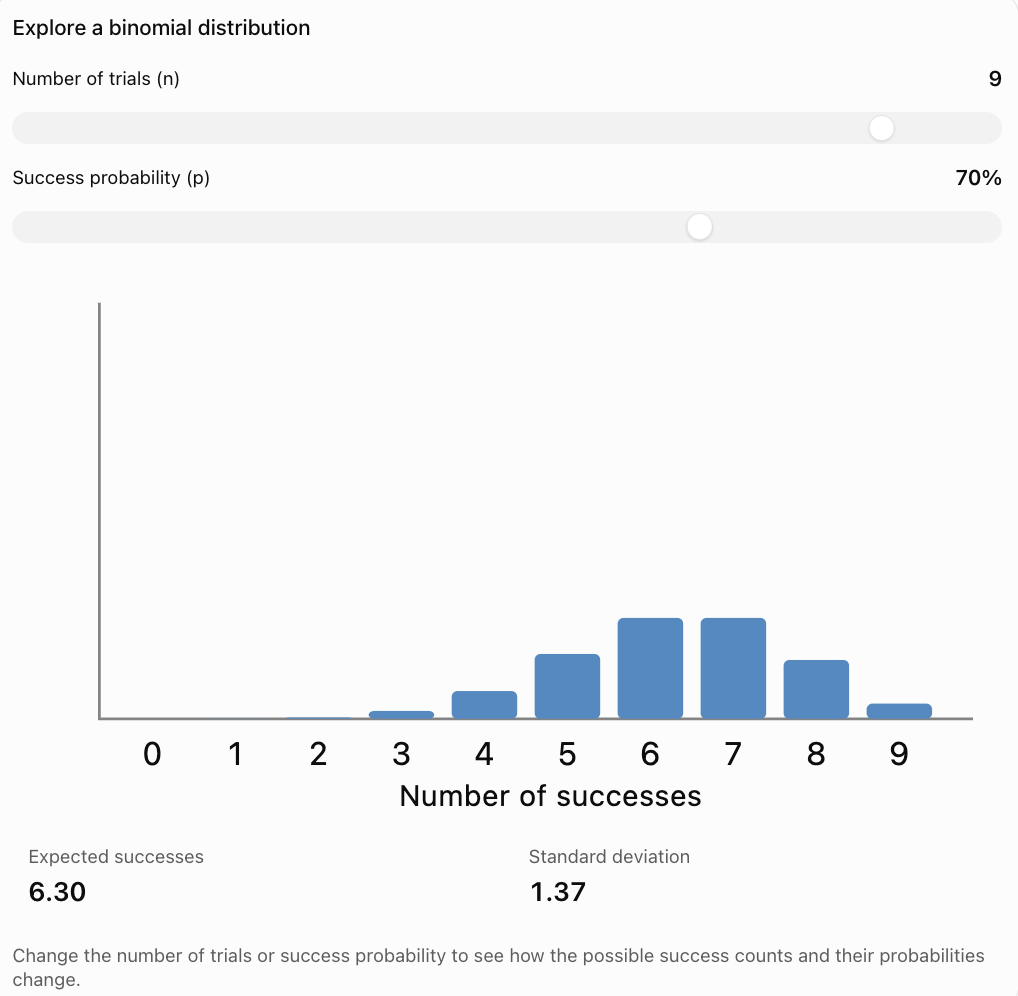
Explore how the distribution changes as the number of trials and probability of success change.

What Happens When p Changes?

When p = 0.5, the distribution is symmetric.

When p is less than 0.5, the distribution tends to be right-skewed.

When p is greater than 0.5, the distribution tends to be left-skewed.

As the number of trials increases, the distribution may begin to resemble a normal distribution, provided neither success nor failure is too rare.

The Binomial Probability Formula

The probability of obtaining exactly k successes in n independent trials is:

P(X = k) = C(n, k) × pᵏ × (1 − p)ⁿ⁻ᵏ

where:

• n = number of trials

• k = number of successes

• p = probability of success

• 1 − p = probability of failure

• C(n, k) = number of ways to choose k successes from n trials

The combination formula is:

C(n, k) = n! / [k!(n − k)!]

The symbol ! represents a factorial.

For example:

5! = 5 × 4 × 3 × 2 × 1 = 120

Also:

0! = 1

Why Does the Formula Work?

The expression:

pᵏ × (1 − p)ⁿ⁻ᵏ

gives the probability of one particular arrangement of k successes and n − k failures.

The expression:

C(n, k)

counts how many different arrangements are possible.

Multiplying them gives the total probability of obtaining exactly k successes.

Worked Example: Tossing Coins

A fair coin is tossed five times.

Find the probability of obtaining exactly three heads.

Step 1: Identify the Values

n = 5

k = 3

p = 0.5

Step 2: Calculate the Number of Combinations

C(5, 3) = 5! / (3!2!)

C(5, 3) = 10

Step 3: Substitute into the Formula

P(X = 3) = 10 × (0.5)³ × (0.5)²

P(X = 3) = 10 × 0.125 × 0.25

P(X = 3) = 0.3125

Final Answer

There is a 31.25% probability of obtaining exactly three heads in five tosses.

Interpretation

If this experiment were repeated many times, approximately 31.25% of the five-toss experiments would produce exactly three heads.

Worked Example: Rolling a Die

A fair six-sided die is rolled four times.

Find the probability of rolling exactly two sixes.

Step 1: Identify the Values

n = 4

k = 2

p = 1/6

1 − p = 5/6

Step 2: Calculate the Combinations

C(4, 2) = 6

Step 3: Apply the Formula

P(X = 2) = 6 × (1/6)² × (5/6)²

P(X = 2) = 6 × (1/36) × (25/36)

P(X = 2) = 150/1296

P(X = 2) ≈ 0.1157

Final Answer

The probability of rolling exactly two sixes is approximately 11.57%.

Calculating Probabilities for Different Outcomes

A binomial distribution can be used to calculate probabilities involving:

• Exactly k successes.

• At least k successes.

• At most k successes.

• More than k successes.

• Fewer than k successes.

These phrases are important because they determine which probabilities must be included.

Calculating At Least a Certain Number of Successes

Suppose a basketball player has an 80% probability of making a free throw.

The player takes five independent shots.

Find the probability of making at least four shots.

Step 1: Identify the Values

n = 5

p = 0.8

We need:

P(X ≥ 4)

Step 2: Identify the Included Outcomes

P(X ≥ 4) = P(X = 4) + P(X = 5)

Step 3: Calculate P(X = 4)

P(X = 4) = C(5, 4)(0.8)⁴(0.2)¹

= 5 × 0.4096 × 0.2

= 0.4096

Step 4: Calculate P(X = 5)

P(X = 5) = C(5, 5)(0.8)⁵

= 0.32768

Step 5: Add

P(X ≥ 4) = 0.4096 + 0.32768

P(X ≥ 4) = 0.73728

Final Answer

There is approximately a 73.73% probability of making at least four out of five shots.

Using Complementary Probability

Sometimes it is easier to calculate the probability of the opposite event.

The complement rule is:

P(A) = 1 − P(not A)

Example: At Least One Success

A fair coin is tossed six times.

Find the probability of obtaining at least one head.

Instead of calculating the probabilities for one, two, three, four, five, and six heads, calculate the probability of no heads.

Step 1: Calculate P(X = 0)

P(X = 0) = (0.5)⁶

P(X = 0) = 0.015625

Step 2: Apply the Complement Rule

P(X ≥ 1) = 1 − P(X = 0)

P(X ≥ 1) = 1 − 0.015625

P(X ≥ 1) = 0.984375

Final Answer

There is a 98.4375% probability of obtaining at least one head in six fair coin tosses.

When Is the Complement Rule Useful?

The complement rule is especially useful for questions involving:

• At least one success.

• At least one failure.

• More than a specified number.

• Fewer than a specified number.

It can greatly reduce the number of calculations.

Expected Value of a Binomial Distribution

The expected value represents the average number of successes expected over many repetitions of the experiment.

For a binomial distribution:

E(X) = np

where:

n = number of trials

p = probability of success

Worked Example

A student guesses on ten multiple-choice questions.

Each question has four options, with one correct answer.

Assume the guesses are independent.

Step 1: Identify the Values

n = 10

p = 1/4 = 0.25

Step 2: Calculate the Expected Value

E(X) = 10 × 0.25

E(X) = 2.5

Interpretation

The student is expected to answer an average of 2.5 questions correctly.

This does not mean the student can answer half a question correctly.

It represents the average number of correct answers across many sets of ten guesses.

Variance of a Binomial Distribution

The variance measures the spread of the number of successes around its expected value.

For a binomial distribution:

Var(X) = np(1 − p)

Since q = 1 − p, the formula may also be written:

Var(X) = npq

Worked Example

A fair coin is tossed twenty times.

Find the variance of the number of heads.

Step 1: Identify the Values

n = 20

p = 0.5

q = 0.5

Step 2: Calculate

Var(X) = 20 × 0.5 × 0.5

Var(X) = 5

Interpretation

The variance describes the spread of the possible numbers of heads around the expected value of 10.

Variance is measured in squared units, which is why standard deviation is often easier to interpret.

Standard Deviation of a Binomial Distribution

The standard deviation is the square root of the variance.

For a binomial distribution:

σ = √[np(1 − p)]

Worked Example

A fair coin is tossed twenty times.

We previously calculated:

Var(X) = 5

Therefore:

σ = √5

σ ≈ 2.24

Interpretation

The number of heads typically varies by an amount on the order of 2.24 from the expected value of 10.

This does not mean that every experiment will produce between 7.76 and 12.24 heads.

Standard deviation measures variability, not a guaranteed interval.

Combining Mean, Variance, and Standard Deviation

Suppose a factory produces items with a 5% probability of being defective.

A sample of 100 items is inspected.

Assume defects occur independently and the defect probability remains constant.

Let X represent the number of defective items.

Step 1: Identify the Distribution

n = 100

p = 0.05

X ~ Bin(100, 0.05)

Step 2: Calculate Expected Value

E(X) = np

E(X) = 100 × 0.05

E(X) = 5

Step 3: Calculate Variance

Var(X) = np(1 − p)

Var(X) = 100 × 0.05 × 0.95

Var(X) = 4.75

Step 4: Calculate Standard Deviation

σ = √4.75

σ ≈ 2.18

Interpretation

The factory expects approximately five defective items per sample of 100.

The standard deviation is approximately 2.18 defective items.

The actual number of defective items will vary between samples.

Understanding How n and p Affect the Distribution

The shape and spread of a binomial distribution depend on n and p.

Effect of Increasing n

When p remains constant and n increases:

• The expected number of successes increases.

• The variance increases.

• The standard deviation increases.

• The relative variation, measured as a fraction of n, generally decreases for 0 < p < 1.

Effect of Changing p

When n remains constant:

• Small p values concentrate probability near zero successes.

• Large p values concentrate probability near n successes.

• p = 0.5 produces a symmetric distribution.

• Variance is largest when p = 0.5.

Example

For n = 10:

The distribution has the greatest variance when success and failure are equally likely.

Binomial Distribution and the Normal Approximation

For sufficiently large n, a binomial distribution can often be approximated using a normal distribution.

A common guideline is:

np ≥ 10

and

n(1 − p) ≥ 10

These conditions help ensure that the distribution is not excessively skewed.

Example

Suppose:

n = 100

p = 0.5

Then:

np = 50

n(1 − p) = 50

Both values exceed 10.

A normal approximation may be appropriate.

Mean and Standard Deviation

The approximating normal distribution has:

Mean = np

Standard deviation = √[np(1 − p)]

Continuity Correction

Because a binomial random variable is discrete and the normal distribution is continuous, a continuity correction can improve the approximation.

For example:

P(X ≤ 20)

is approximated using:

P(Y ≤ 20.5)

where Y is the corresponding normal random variable.

This is an extension of the basic binomial model.

Real-World Application: Manufacturing Quality Control

Manufacturers use binomial probability models to analyse defective products.

Example

A factory estimates that 3% of its products are defective.

A quality-control inspector randomly selects twenty products.

Assume independent outcomes with constant defect probability.

Let X represent the number of defective products.

X ~ Bin(20, 0.03)

Expected Number of Defects

E(X) = 20 × 0.03

E(X) = 0.6

Probability of No Defects

P(X = 0) = (0.97)²⁰

P(X = 0) ≈ 0.5438

Interpretation

There is approximately a 54.38% probability that none of the twenty selected products will be defective.

Although the expected number of defects is only 0.6, the sample may contain zero, one, or several defective items.

Real-World Application: Medical Testing

Binomial distributions can model the number of positive test results under suitable assumptions.

Example

Suppose a screening programme tests 50 independent samples.

Assume each sample has a 10% probability of testing positive.

Let X represent the number of positive results.

X ~ Bin(50, 0.10)

Expected Value

E(X) = 50 × 0.10

E(X) = 5

Variance

Var(X) = 50 × 0.10 × 0.90

Var(X) = 4.5

Standard Deviation

σ = √4.5

σ ≈ 2.12

Interpretation

The expected number of positive results is five.

The actual number may vary between samples.

In real medical testing, independence and constant probability may not always be appropriate. Test accuracy and the population being tested also matter.

Real-World Application: Sports Performance

Binomial models can help analyse repeated sports attempts.

Example

A basketball player makes 75% of free throws.

Assume independent attempts with a constant success probability.

The player takes eight shots.

Find the probability of making exactly six.

Step 1: Identify the Values

n = 8

p = 0.75

k = 6

Step 2: Apply the Formula

P(X = 6) = C(8, 6)(0.75)⁶(0.25)²

C(8, 6) = 28

P(X = 6) = 28 × 0.1779785 × 0.0625

P(X = 6) ≈ 0.3115

Final Answer

There is approximately a 31.15% probability of making exactly six out of eight free throws.

Real-World Application: Education

Teachers can use binomial probability to investigate guessing on multiple-choice examinations.

Example

A student guesses randomly on twelve questions.

Each question has four options, with one correct answer.

Assume independent guesses.

Distribution

n = 12

p = 0.25

X ~ Bin(12, 0.25)

Expected Correct Answers

E(X) = 12 × 0.25

E(X) = 3

Probability of Getting All Questions Wrong

P(X = 0) = (0.75)¹²

P(X = 0) ≈ 0.0317

Interpretation

There is approximately a 3.17% probability of getting every question wrong through random guessing.

The expected number of correct answers is three.

Common Mistakes

Assuming every repeated experiment is binomial

All four BINS conditions must be satisfied.

Forgetting that trials must be independent

Dependent trials may require a different probability model.

Using the wrong success probability

The value of p must correspond to the event defined as success.

Confusing n and k

n is the total number of trials.

k is the number of successes.

Forgetting the combination term

C(n, k) counts the possible arrangements of successes.

Using p instead of 1 − p for failures

The failure probability is q = 1 − p.

Confusing exactly with at least

Exactly three means X = 3.

At least three means X ≥ 3.

Adding probabilities incorrectly

Events representing different possible numbers of successes must be combined correctly.

Forgetting the complement rule

Sometimes calculating the opposite event is much easier.

Confusing expected value with probability

Expected value is a number of successes, not a probability.

Using the wrong variance formula

Variance = np(1 − p), not np.

Forgetting the square root for standard deviation

Standard deviation = √[np(1 − p)].

Assuming expected value must be a whole number

Expected value may be fractional.

Applying a normal approximation without checking conditions

The approximation may be inaccurate when n is small or p is close to 0 or 1.

Key Terms

• Binomial Experiment: Experiment with a fixed number of independent binary trials and constant success probability.

• Binomial Distribution: Discrete probability distribution describing the number of successes in a binomial experiment.

• Trial: Single repetition of an experiment.

• Success: Outcome designated as the event of interest.

• Failure: Outcome that is not classified as success.

• Independent Trials: Trials whose outcomes do not affect one another's probabilities.

• Probability of Success (p): Probability that a trial produces a success.

• Probability of Failure (q): Probability that a trial produces a failure, where q = 1 − p.

• Number of Trials : Total number of repetitions.

• Number of Successes (k): Number of successful outcomes.

• Combination: Number of ways to select objects or positions without regard to order.

• Factorial: Product of positive integers from 1 to a specified integer.

• Binomial Coefficient: Number C(n, k) of ways to choose k successes from n trials.

• Probability Mass Function: Function assigning probabilities to discrete values.

• Expected Value: Long-run average number of successes.

• Variance: Measure of the spread of the distribution around its mean.

• Standard Deviation: Square root of variance.

• Complementary Probability: Probability of an event not occurring.

• Cumulative Probability: Probability of obtaining at most a specified number of successes.

• Symmetric Distribution: Distribution with balanced left and right sides.

• Skewed Distribution: Distribution with an extended tail on one side.

• Normal Approximation: Use of a normal distribution to approximate a binomial distribution.

• Continuity Correction: Adjustment used when approximating discrete probabilities with a continuous distribution.

Key Takeaways

• Binomial experiments satisfy the four BINS conditions.

• Each trial has two possible outcomes: success or failure.

• The number of trials must be fixed.

• Trials must be independent.

• The probability of success must remain constant.

• A binomial random variable counts the number of successes.

• Binomial notation is X ~ Bin(n, p).

• The binomial probability formula is P(X = k) = C(n, k)pᵏ(1 − p)ⁿ⁻ᵏ.

• The expected value is E(X) = np.

• The variance is Var(X) = np(1 − p).

• The standard deviation is σ = √[np(1 − p)].

• The complement rule simplifies many probability calculations.

• A binomial distribution is symmetric when p = 0.5.

• The distribution becomes increasingly skewed as p moves toward 0 or 1.

• Binomial models are useful in manufacturing, medicine, sports, education, and scientific research.

• The model should only be used when its assumptions are appropriate.

Check Your Understanding

Identifying Binomial Experiments

1. State the four conditions required for a binomial experiment.

2. Explain why tossing a fair coin ten times is binomial.

3. Explain why drawing cards without replacement is generally not exactly binomial.

4. Is counting the number of sixes in eight independent die rolls binomial?

5. Is measuring the heights of twenty students binomial?

Calculating Binomial Probabilities

6. Write the binomial probability formula.

7. Calculate C(5, 2).

8. A fair coin is tossed four times. Find P(X = 2).

9. A fair die is rolled three times. Find the probability of obtaining no sixes.

10. A player has a 60% probability of success. Find the probability of exactly two successes in three independent attempts.

Expected Value

11. Calculate E(X) for n = 20 and p = 0.4.

12. Calculate E(X) for n = 50 and p = 0.1.

13. Explain why the expected value may not be a whole number.

14. A student guesses on 16 four-option multiple-choice questions. Find the expected number correct.

15. A factory has a 2% defect rate. Find the expected number of defects in 200 independently produced items.

Variance and Standard Deviation

16. Write the formula for binomial variance.

17. Calculate the variance for n = 10 and p = 0.5.

18. Calculate the standard deviation for n = 10 and p = 0.5.

19. Calculate the variance for n = 40 and p = 0.2.

20. Explain what standard deviation tells us about a binomial distribution.

Answer Key

Extended Challenge

Binomial Identification

1. A student tosses a coin until the first head appears. Explain why this is not a binomial experiment.

2. A factory inspects twenty products selected independently from a very large production process. Explain when a binomial model would be appropriate.

3. A basketball player attempts ten free throws. Discuss the assumptions needed to use a binomial model.

4. Explain why rolling a die can produce a binomial experiment even though a die has six possible outcomes.

5. Describe a real-world experiment that satisfies all four BINS conditions.

Probability Calculations

6. A fair coin is tossed eight times. Find the probability of exactly five heads.

7. A fair die is rolled six times. Find the probability of exactly two sixes.

8. A player has a 70% success rate. Find the probability of exactly four successes in six independent attempts.

9. A factory has a 4% defect rate. Find the probability of no defective items in a sample of fifteen independent items.

10. A student guesses on ten four-option multiple-choice questions. Find the probability of answering at least one correctly.

Expected Value and Variability

11. Calculate the expected value for n = 60 and p = 0.3.

12. Calculate the variance for the same distribution.

13. Calculate the standard deviation.

14. Explain what happens to expected value when n doubles but p remains constant.

15. Explain why variance is greatest when p = 0.5 for a fixed n.

Practical Applications

16. A hospital estimates that 8% of patients will require a particular follow-up appointment. Find the expected number requiring follow-up among 100 independent patients.

17. Calculate the variance and standard deviation for the same situation.

18. A football player has a 65% probability of scoring a penalty. Find the probability of scoring at least three out of four independent penalties.

19. Explain why a binomial model might not be appropriate if a player's success probability changes due to fatigue.

20. Describe how binomial probabilities can help businesses make decisions under uncertainty.

Final Investigation: Quality Control in a Factory

A factory produces electronic components.

The probability that a component is defective is 0.05.

A quality-control inspector randomly selects twenty components.

Assume the selected components have independent defect outcomes and the probability of a defect remains constant.

Let X represent the number of defective components.

Complete the investigation.

1. Explain why this situation can be modelled using a binomial distribution.

2. Identify n.

3. Identify p.

4. Identify q.

5. Write the binomial notation for X.

6. Calculate the probability of finding no defective components.

7. Calculate the probability of finding exactly one defective component.

8. Calculate the probability of finding exactly two defective components.

9. Calculate the probability of finding at least one defective component.

10. Calculate the probability of finding at most two defective components.

11. Calculate the expected number of defective components.

12. Calculate the variance.

13. Calculate the standard deviation.

14. Construct a probability distribution table for X = 0 through X = 5.

15. Construct a bar graph for these probabilities.

16. Describe the shape of the distribution.

17. Explain why the expected number of defective components is not necessarily the most likely observed number.

18. Discuss whether a normal approximation would be appropriate.

19. Explain how the factory could use this model to plan quality-control inspections.

20. Write a conclusion explaining the usefulness and limitations of the binomial distribution in manufacturing.