Quadratic Modelling with Technology

Introduction

Mathematical models help us identify patterns, describe relationships, and make predictions from real-world data.

When data follows a curved pattern, a quadratic function may provide a useful model. Graphing technology allows us to analyse these relationships more efficiently than performing every calculation by hand.

Tools such as graphing calculators, spreadsheets, Desmos, and GeoGebra can help us:

• Organise and graph measured data.

• Identify patterns in scatter plots.

• Calculate quadratic regression equations.

• Compare predicted values with actual observations.

• Find maximum and minimum values.

• Evaluate the accuracy and limitations of a model.

• Make predictions about future or unknown values.

Quadratic modelling is especially useful in physics, engineering, economics, environmental science, and other fields where quantities change at a nonconstant rate.

What Is Mathematical Modelling?

A mathematical model is an equation, graph, table, or other mathematical representation used to describe a real-world relationship.

For example, a model might describe:

• The height of a projectile over time.

• The relationship between a vehicle's speed and braking distance.

• The area of a garden as its dimensions change.

• The revenue earned by a business at different selling prices.

• The relationship between production quantity and manufacturing costs.

A model simplifies a situation so that mathematical methods can be used to analyse it.

Important Observation

A mathematical model is not necessarily an exact description of reality. It is a representation based on available data and assumptions.

Recognising Quadratic Relationships in Data

A quadratic function has the general form:

y = ax² + bx + c

where a ≠ 0.

Its graph is a parabola.

Quadratic relationships often appear when:

• Data increases and then decreases.

• Data decreases and then increases.

• A quantity has a maximum or minimum.

• The rate of change varies in a roughly linear way.

• A relationship involves the square of a variable.

Example

A ball is launched upward, and its height is measured at different times.

The height increases, reaches a maximum, and then decreases.

This pattern suggests a downward-opening parabola.

A quadratic function is therefore a reasonable model to investigate.

Using Scatter Plots

A scatter plot displays pairs of numerical data as points on a coordinate plane.

Each point represents one observation.

For example:

(0, 0)

(1, 15)

(2, 20)

(3, 15)

(4, 0)

Why Use a Scatter Plot?

Scatter plots help us:

• Identify curved or linear patterns.

• Detect unusual measurements.

• Observe possible maximum and minimum values.

• Compare measured data with a mathematical model.

• Decide which type of regression may be appropriate.

Important Observation

A scatter plot displays actual observations. A regression curve represents a mathematical model fitted to those observations.

The curve does not necessarily pass through every point.

Quadratic Regression

Quadratic regression is a statistical technique used to find a quadratic equation that best fits a set of data.

The model has the form:

ŷ = ax² + bx + c

The symbol ŷ represents a predicted value.

Graphing technology calculates values for a, b, and c that make the model fit the observations as closely as possible according to a selected fitting method.

Most standard quadratic regression tools use least squares regression.

This method minimises the sum of the squared vertical differences between observed and predicted values.

Example

Suppose graphing technology produces:

ŷ = −4.8x² + 19.5x + 1.2

This could represent the height of a projectile.

The coefficients have mathematical meanings:

• a = −4.8 controls the curvature and indicates a downward-opening parabola.

• b = 19.5 represents the initial rate of change in the model.

• c = 1.2 represents the predicted height when x = 0.

Important Observation

Regression finds a model from data. The coefficients are estimates and may differ slightly from the values expected from a theoretical equation.

How Least Squares Regression Works

Suppose a quadratic model predicts a height of 12 metres, but the measured height is 11.5 metres.

The difference is called a residual.

Residual = observed value − predicted value

Residual = 11.5 − 12

Residual = −0.5 m

The squared residual is:

(−0.5)² = 0.25

For a set of observations, least squares regression chooses the coefficients that minimise:

SSE = Σ(observed − predicted)²

where SSE means sum of squared errors.

Why Square the Residuals?

Squaring:

• Prevents positive and negative residuals from cancelling.

• Gives larger errors greater influence.

• Produces a mathematical quantity that can be minimised.

Important Observation

A regression equation is generally an approximation, not a perfect equation through all measured points.

Creating a Quadratic Regression Model

Consider the following experimental data.

The values suggest that the object rises and then falls.

A suitable approximate model is:

h(t) = −5t² + 20t + 1

Comparing the Model with Observations

This equation is a simple illustrative model, not the exact least-squares regression result.

The differences between observed and predicted heights are small, suggesting that the model describes these measurements reasonably well.

Exploring the Fit of a Quadratic Model

The following graph shows the measured data and the illustrative quadratic model.

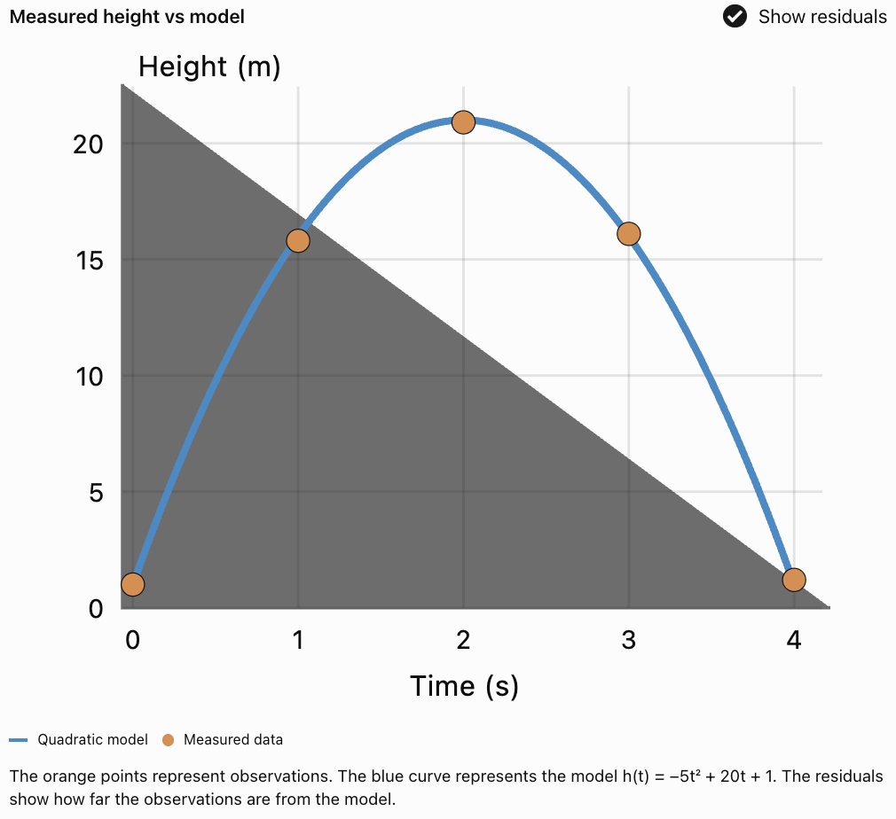
Interpretation

Most measured points lie close to the curve.

This suggests that a quadratic model is appropriate for the observed time interval.

However, a close fit does not guarantee that the model will remain accurate outside that interval.

Using Desmos for Quadratic Regression

Open Desmos Graphing Calculator

Desmos provides a convenient way to create scatter plots and perform regression.

Procedure

1. Open the Desmos Graphing Calculator.

2. Select Add Item, then Table.

3. Enter the independent-variable values in the first column.

4. Enter the dependent-variable values in the second column.

5. Create a new expression using the table column names.

For a standard table named x₁ and y₁, enter:

y₁ ~ ax₁² + bx₁ + c

The tilde symbol (~) tells Desmos to perform regression.

Desmos calculates values for a, b, and c.

What to Examine

After calculating the regression:

• Record the equation.

• Examine the shape of the fitted curve.

• Identify the vertex.

• Compare the curve with the observed points.

• Examine the residuals.

• Decide whether the model makes sense in context.

Important Observation

In Desmos, the regression expression uses ~ rather than = because the software is estimating coefficients from measured data.

Using GeoGebra for Quadratic Regression

Open GeoGebra Graphing Calculator

GeoGebra can also be used to analyse quadratic relationships.

General Procedure

1. Enter the observed data as points.

2. Display the points on the coordinate plane.

3. Create a list of the points.

4. Use a quadratic polynomial fitting command such as FitPoly(list, 2), with the actual point-list name substituted for list.

5. Display the resulting quadratic equation.

6. Compare the fitted curve with the observed points.

Important Observation

Different graphing tools may display equations or coefficients with slightly different rounding.

When the same data and least-squares method are used, the underlying results should be consistent.

Using Spreadsheets for Quadratic Modelling

Spreadsheet programs such as Excel and Google Sheets can also perform quadratic regression.

General Procedure

1. Enter x-values in one column.

2. Enter y-values in another column.

3. Create an XY scatter chart.

4. Add a trendline.

5. Select a polynomial trendline.

6. Set the polynomial order to 2.

7. Display the equation and R² value if the software supports these options.

Important Observation

A polynomial trendline of order 2 represents a quadratic function.

An order-1 polynomial represents a linear function.

Interpreting Regression Coefficients

Suppose the regression equation is:

ŷ = −2.5x² + 15x + 8

Coefficient a

a = −2.5

The parabola opens downward.

The model has a maximum.

Coefficient b

b = 15

This affects the position of the vertex and the rate of change.

In a model where x represents time, it may represent an initial rate of change.

Coefficient c

c = 8

The predicted value when x = 0 is 8.

Finding the Vertex

x = −b/(2a)

x = −15/[2(−2.5)]

x = 3

Substitute:

ŷ = −2.5(3)² + 15(3) + 8

ŷ = −22.5 + 45 + 8

ŷ = 30.5

Interpretation

The model predicts a maximum value of 30.5 when x = 3.

The real-world meaning depends on the variables and units.

Understanding the Coefficient of Determination

Graphing technology may report a value called R², known as the coefficient of determination.

For ordinary regression with an intercept, it is commonly calculated as:

R² = 1 − SSE/SST

where:

• SSE = sum of squared residuals.

• SST = sum of squared differences between observed values and their mean.

Interpreting R²

These are illustrative interpretations, not universal thresholds. Whether a fit is acceptable depends on the subject, measurement accuracy, and purpose of the model.

Example

Suppose:

R² = 0.96

This indicates that approximately 96% of the variation in the observed dependent variable is accounted for by the fitted model, using the usual R² definition.

Important Observation

A high R² does not prove that a model is correct, that the relationship is causal, or that future predictions will be accurate.

Comparing Predicted and Observed Values

After creating a regression equation, compare its predictions with actual measurements.

Example

Suppose a model predicts:

ŷ = 2x² + 3x + 1

At x = 2:

ŷ = 2(2)² + 3(2) + 1

ŷ = 8 + 6 + 1

ŷ = 15

If the observed value is 14.5:

Residual = 14.5 − 15

Residual = −0.5

Interpretation

The model overestimated the observation by 0.5 units.

A table of residuals can help determine whether the model consistently overestimates or underestimates particular regions of the data.

Residual Plots

A residual plot displays residuals against the independent variable.

Residual plots are useful for detecting patterns that may not be obvious from the original scatter plot.

A Suitable Model

If residuals are scattered approximately randomly around zero, the model may describe the data reasonably well.

An Unsuitable Model

If residuals form a systematic curve or trend, the chosen model may be missing an important pattern.

Other Warning Signs

• Residuals become larger as x increases.

• One or two points have unusually large residuals.

• Residuals remain mostly positive or mostly negative over a long interval.

Important Observation

A residual plot can reveal problems even when the original regression curve appears to fit the data well.

Making Predictions Using a Quadratic Model

Once a suitable model has been developed, it can be used to estimate values that were not directly measured.

Worked Example

Suppose a quadratic regression model for a projectile is:

h(t) = −4.9t² + 19.6t + 1.5

where:

• t = time in seconds

• h = height in metres

Find the predicted height after 1.5 seconds.

Step 1: Substitute the Time

h(1.5) = −4.9(1.5)² + 19.6(1.5) + 1.5

Step 2: Calculate

h(1.5) = −4.9(2.25) + 29.4 + 1.5

h(1.5) = −11.025 + 29.4 + 1.5

h(1.5) = 19.875 m

Interpretation

The model predicts a height of approximately 19.9 metres after 1.5 seconds.

This is a prediction, not necessarily an exact measured height.

Predicting Maximum and Minimum Values

A quadratic regression equation can also be used to estimate maximum or minimum values.

For:

y = ax² + bx + c

the x-coordinate of the vertex is:

x = −b/(2a)

Example

A company's profit is modelled by:

P(x) = −2x² + 48x − 100

where x represents the number of products sold and P is measured in dollars.

Find the Optimal Quantity

x = −48/[2(−2)]

x = 12

Find the Maximum Profit

P(12) = −2(12)² + 48(12) − 100

P(12) = −288 + 576 − 100

P(12) = $188

Interpretation

The model predicts a maximum profit of $188 when 12 products are sold.

Important Observation

The vertex gives the optimum of the quadratic equation, but the answer must still satisfy the practical constraints of the situation.

Interpolation and Extrapolation

Predictions can be classified into two categories.

Interpolation

Interpolation involves predicting a value within the range of observed data.

Suppose measurements were collected for:

0 ≤ t ≤ 5 seconds

Predicting the value at t = 2.5 seconds is interpolation.

This is generally more reliable because the prediction lies within the measured interval.

Extrapolation

Extrapolation involves predicting a value outside the observed data range.

Using the same measurements to predict the value at t = 15 seconds is extrapolation.

This is generally less reliable because the relationship may change beyond the measured interval.

Example

A projectile model may predict a negative height long after the projectile has landed.

Although the equation can be evaluated mathematically, the result does not describe the object's actual position after impact.

Important Conclusion

A model should only be used for predictions within a range where its assumptions and behaviour remain reasonable.

Comparing Linear and Quadratic Regression

Graphing technology allows us to compare different models fitted to the same data.

Consider:

First Differences

2, 4, 6, 8

These are not constant.

Second Differences

2, 2, 2

These are constant.

The data follow an exact quadratic pattern.

A suitable equation is:

y = x² + x + 2

Comparing Models

A linear regression model would produce a straight line that does not pass through all five points.

The quadratic model passes through every point.

Important Observation

A quadratic model may fit curved data better than a linear model, but greater complexity is not always desirable. Models should be selected based on accuracy, simplicity, physical reasoning, and their ability to predict new observations.

Limitations of Quadratic Regression

Quadratic regression is powerful, but it has limitations.

Measurement Error

Real-world measurements may contain errors caused by instruments, human observation, or environmental conditions.

Limited Data

A model based on only a few measurements may not reliably represent the full relationship.

In particular, three distinct x-values can determine an exact quadratic equation even if the data do not come from a genuinely quadratic process.

Outliers

An unusually high or low observation can influence the fitted curve.

Incorrect Model Type

Some relationships are exponential, logarithmic, periodic, or more complicated than a quadratic function.

Restricted Domains

A model may only apply over a particular range of inputs.

Changing Conditions

Real-world conditions may change after data collection.

For example, production costs, weather conditions, or physical forces may vary.

Correlation Does Not Establish Causation

A quadratic relationship between two variables does not automatically mean that one variable causes changes in the other.

Evaluating the Quality of a Model

A useful quadratic model should satisfy several criteria.

Important Observation

No single statistic is sufficient to determine whether a model is appropriate.

A strong evaluation considers both mathematical accuracy and real-world meaning.

Improving a Quadratic Model

If a model does not fit the observations well, several improvements may be possible.

• Collect more measurements across the relevant input range.

• Check for recording or measurement errors.

• Investigate unusually large residuals.

• Use more precise measuring instruments.

• Compare quadratic regression with other model types.

• Restrict the model to a range where the relationship is valid.

• Test predictions against new observations.

Example

Suppose a quadratic model describes the first five seconds of a ball's motion accurately but becomes unrealistic after the ball lands.

Rather than extending the same equation indefinitely, restrict the model to the time interval during which the ball is actually in flight.

Real-World Applications of Quadratic Regression

Physics

Experimental height-time data can be used to estimate projectile motion.

Transportation

Vehicle-speed and braking-distance measurements can be analysed using quadratic models.

Business

Sales and revenue data can be used to estimate optimal production quantities or prices.

Engineering

Measured points on curved structures can be used to fit parabolic models.

Agriculture

Data relating planting dimensions to area or production can be analysed to identify useful mathematical relationships.

Important Observation

The value of quadratic regression comes from combining mathematical techniques with meaningful data and appropriate interpretation.

Common Mistakes

Assuming regression produces an exact equation

Regression usually produces an approximation based on measured data.

Confusing observed and predicted values

Observed values come from measurements. Predicted values come from the model.

Ignoring residuals

A curve may appear accurate while still producing systematic prediction errors.

Assuming R² = 1 proves a model is physically correct

A perfect fit to existing observations does not guarantee a correct underlying explanation.

Choosing quadratic regression for every curved pattern

Not all nonlinear relationships are quadratic.

Extrapolating too far

Predictions outside the observed range may be unreliable.

Ignoring units

Every coefficient and prediction must be interpreted in the context of the variables.

Rounding coefficients too early

Premature rounding can introduce errors into calculated predictions.

Ignoring outliers

Unusual measurements may significantly influence the regression equation.

Using unrealistic input values

A model may produce mathematically valid outputs that are impossible in the real situation.

Key Terms

• Mathematical Model: Mathematical representation of a real-world relationship.

• Quadratic Model: Model expressed using a quadratic function.

• Quadratic Regression: Statistical method for fitting a quadratic equation to data.

• Scatter Plot: Graph displaying paired numerical observations.

• Regression Curve: Curve fitted to observed data.

• Least Squares: Method that minimises the sum of squared residuals.

• Observed Value: Value obtained from actual measurement.

• Predicted Value: Value calculated using a mathematical model.

• Residual: Difference between an observed and predicted value.

• Sum of Squared Errors (SSE): Sum of squared residuals.

• Coefficient of Determination (R²): Statistic describing the proportion of observed variation accounted for by a fitted model under the usual definition.

• Residual Plot: Graph showing residuals against input values or predictions.

• Outlier: Observation unusually far from the overall pattern.

• Interpolation: Prediction within the observed data range.

• Extrapolation: Prediction outside the observed data range.

• Independent Variable: Input variable.

• Dependent Variable: Output variable.

• Vertex: Maximum or minimum point of a parabola.

• Domain: Set of permitted input values.

• Range: Set of possible output values.

• Trendline: Line or curve fitted to data to represent a pattern.

• Polynomial Regression: Regression using a polynomial function.

• Measurement Error: Difference between a measurement and the actual quantity.

• Model Limitation: Condition restricting the accuracy or usefulness of a model.

Key Takeaways

• Graphing technology makes it easier to analyse real-world numerical data.

• Scatter plots help identify relationships between variables.

• Quadratic regression fits a parabola to measured data.

• A quadratic regression equation has the form ŷ = ax² + bx + c.

• The coefficients describe the shape and position of the fitted parabola.

• Least squares regression minimises the sum of squared residuals.

• Residuals measure differences between observed and predicted values.

• Residual plots help identify patterns that a model may fail to explain.

• R² provides information about how closely a model fits the observed data.

• A high R² does not guarantee that the model is correct.

• The vertex can be used to estimate maximum or minimum values.

• Quadratic models can be used for interpolation and extrapolation.

• Extrapolation is generally less reliable.

• A model should be evaluated using mathematical accuracy, physical meaning, and appropriate assumptions.

• Technology supports mathematical reasoning but does not replace interpretation.

Check Your Understanding

Understanding Quadratic Regression

1. What is quadratic regression?

2. What is the purpose of a scatter plot?

3. What does the symbol ŷ represent?

4. Why does least squares regression square the residuals?

5. What does a negative coefficient a indicate about the fitted parabola?

Interpreting Regression Results

6. A regression equation is ŷ = −2x² + 12x + 5. What is the predicted value when x = 0?

7. Determine the vertex of the equation in Question 6.

8. Does the equation have a maximum or minimum?

9. What does R² measure?

10. Does a high R² prove that a quadratic model is correct?

Comparing Models with Data

11. Define a residual.

12. Calculate the residual when the observed value is 18 and the predicted value is 20.

13. What does a positive residual indicate?

14. Why are residual plots useful?

15. What might a systematic curved pattern in residuals suggest?

Predictions and Limitations

16. Explain the difference between interpolation and extrapolation.

17. Why is extrapolation generally less reliable?

18. Give one reason a quadratic model might produce unrealistic predictions.

19. Why should units be included when interpreting regression results?

20. Name two technologies that can perform quadratic regression.

Answer Key

Extended Challenge

1. A regression equation is ŷ = −3x² + 24x + 10. Determine the vertex.

2. Interpret the maximum value if y represents height in metres and x represents time in seconds.

3. Use the model in Question 1 to predict the height at x = 2.

4. Find the positive x-intercept of the model in Question 1.

5. A quadratic model predicts 35.2, but the observed value is 34.7. Calculate the residual.

6. Explain why a model with R² = 0.98 might still be inappropriate for long-term predictions.

7. Construct a quadratic equation through the points (0, 2), (1, 5), and (2, 10).

8. Explain why fitting exactly three points is not sufficient evidence that the real-world relationship is quadratic.

9. Compare the advantages of quadratic regression and manually fitting a parabola.

10. Describe how you would evaluate whether a quadratic model is more appropriate than a linear model for an experimental dataset.

Final Investigation: Modelling Projectile Data with Technology

A student records the height of a ball at different times during a projectile experiment.

The following measurements are collected:

Investigation Tasks

1. Identify the independent variable.

2. Identify the dependent variable.

3. Enter the data into Desmos, GeoGebra, or a spreadsheet.

4. Create a scatter plot.

5. Describe the pattern of the observations.

6. Explain why quadratic regression may be appropriate.

7. Calculate the quadratic regression equation using technology.

8. Record the coefficients a, b, and c.

9. Explain what the sign of a indicates.

10. Graph the regression curve alongside the measured points.

11. Record the R² value if available.

12. Calculate the predicted height at t = 1 second.

13. Calculate the predicted height at t = 2 seconds.

14. Find the residuals for the measurements at t = 1 and t = 2.

15. Create a residual plot.

16. Determine the predicted time at maximum height.

17. Calculate the predicted maximum height.

18. Estimate when the ball reaches ground level.

19. Identify two limitations of the model.

20. Write a conclusion evaluating how effectively quadratic regression describes the experimental data.

Investigation Guidance

A successful investigation should include:

• A labelled scatter plot.

• A quadratic regression equation.

• A graph of the fitted parabola.

• Calculated predictions and residuals.

• The estimated vertex.

• An explanation of the model's accuracy.

• A discussion of assumptions and limitations.

Extension

Use the fitted equation to predict the ball's height at t = 5 seconds.

Explain whether the prediction is physically meaningful and whether it should be trusted.

Consider whether the ball would already have reached the ground.