Equations of Motion
5. Real-World Applications
Learning outcomes
- I can apply kinematic equations to real-world situations.
- I can analyze motion in transportation, sports, and engineering contexts.
- I can interpret motion data using equations and graphs.
- I can model physical situations using the equations of motion.
- I can explain how kinematics is used to solve practical problems.
What is a kinematic model?
A kinematic model is a mathematical description of an object’s motion. It connects quantities such as:
- Position and displacement.
- Distance travelled.
- Speed and velocity.
- Acceleration.
- Time.
Kinematic models allow us to predict where an object will be, how fast it will move and how long a motion will take.
They are used in:
- Vehicle design and road safety.
- Sports training and performance analysis.
- Roller-coaster and elevator design.
- Robotics and automated manufacturing.
- Aircraft and spacecraft navigation.
- Accident reconstruction.
- Motion sensors and tracking systems.
A model is a simplified representation of reality. Its usefulness depends on whether its assumptions are reasonable.
Selecting a motion model
Before using an equation, decide how the object is moving.
Constant velocity
Use a constant-velocity model when speed and direction remain unchanged:
s = vt
or:
x = x₀ + vt
Uniform acceleration
Use the equations of motion when acceleration remains constant:
v = u + at
s = ½(u + v)t
s = ut + ½at²
v² = u² + 2as
s = vt − ½at²
Changing acceleration
If acceleration varies significantly, a single constant-acceleration equation may not represent the entire motion.
Possible approaches include:
- Dividing the motion into shorter stages.
- Interpreting experimental graphs.
- Estimating areas and gradients.
- Using calculus or computer simulations.
- Collecting additional motion data.
From reality to a mathematical model
A practical kinematics problem can be organized into the following sequence:
- Identify the object and the interval of motion.
- Choose an origin and positive direction.
- Decide whether velocity or acceleration is constant.
- Identify the known and unknown quantities.
- Select an appropriate equation or graph method.
- Calculate the required quantity.
- Interpret the result in context.
- Evaluate the model’s assumptions and limitations.
For example, a braking car might be simplified as an object moving in a straight line with constant negative acceleration. This model ignores small changes in braking force and road conditions but can still provide a useful estimate.
Transportation: reaction and braking distances
A vehicle does not stop immediately when a driver notices a hazard.
Total stopping distance has two parts:
Total stopping distance = thinking distance + braking distance
Thinking distance
Thinking distance is the distance travelled during the driver’s reaction time.
If the vehicle travels at constant velocity during this brief interval:
Thinking distance = initial speed × reaction time
dₜ = utᵣ
Thinking distance increases directly with speed when reaction time remains constant.
Braking distance
After the brakes are applied, the vehicle decelerates.
For a simplified constant-deceleration model:
v² = u² + 2as
When the vehicle stops, v = 0. If d represents the positive magnitude of deceleration:
0 = u² − 2ds
Therefore:
Braking distance = u²/(2d)
Braking distance depends on the square of the initial speed.
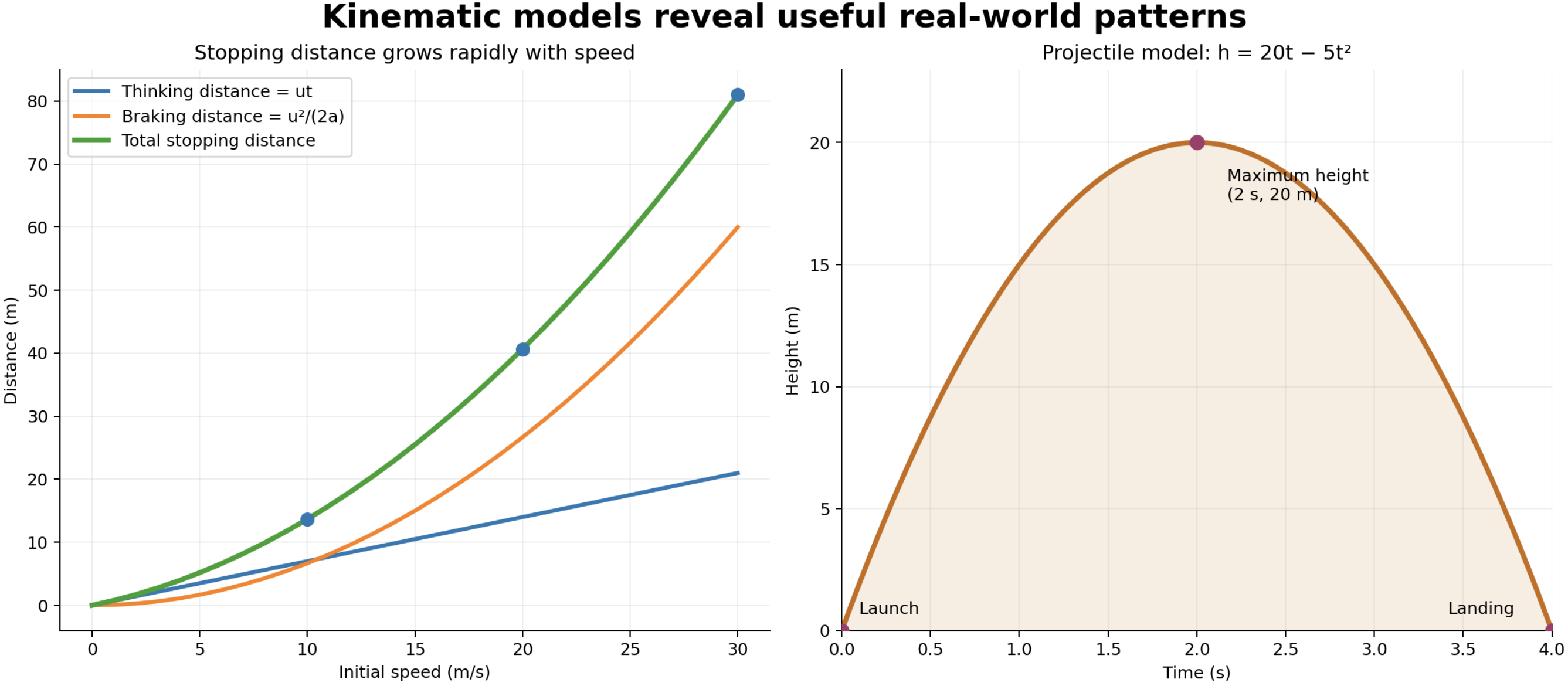
In the stopping model, reaction time is 0.7 s and the braking deceleration has magnitude 7.5 m/s². Thinking distance grows linearly with speed, while braking distance grows quadratically.
Worked example: vehicle stopping distance
A car travels at 20 m/s. The driver’s reaction time is 0.7 s, and the car then brakes uniformly with a deceleration magnitude of 7.5 m/s².
Thinking distance
dₜ = utᵣ
dₜ = 20(0.7)
dₜ = 14 m
Braking distance
Use:
v² = u² + 2as
Choose the direction of travel as positive:
u = 20 m/s
v = 0 m/s
a = −7.5 m/s²
Substitute:
0² = 20² + 2(−7.5)s
0 = 400 − 15s
15s = 400
s ≈ 26.7 m
Total stopping distance
Total distance = 14 + 26.7
Total distance ≈ 40.7 m
The car travels approximately 41 m between the driver seeing the hazard and the vehicle stopping.
Why higher speed greatly increases stopping distance
Suppose braking conditions remain unchanged.
At 10 m/s:
Braking distance = 10²/(2 × 7.5)
Braking distance ≈ 6.7 m
At 20 m/s:
Braking distance = 20²/(2 × 7.5)
Braking distance ≈ 26.7 m
Doubling the initial speed increases the braking distance by a factor of four.
This occurs because:
Braking distance ∝ speed²
The total stopping distance does not increase by exactly four because thinking distance depends directly on speed rather than speed squared.


Real braking distance depends on tyre condition, road surface, weather, brakes, vehicle mass distribution and driver response. The equation gives a model based on the stated acceleration.
Interpreting braking data from a velocity–time graph
A velocity–time graph can show a vehicle’s complete stopping process.
- A horizontal section represents the reaction interval.
- A downward-sloping section represents braking.
- The gradient during braking gives acceleration.
- The complete area under the graph gives stopping distance.
Suppose a car remains at 18 m/s for 0.8 s and then slows uniformly to rest in 3.0 s.
Thinking distance:
d = 18(0.8)
d = 14.4 m
Braking distance:
d = ½(3.0)(18)
d = 27 m
Total stopping distance:
d = 14.4 + 27
d = 41.4 m
The graphical and equation-based methods describe the same motion.
Transportation: journey planning
Constant-velocity equations can estimate travel time over a steady section of a journey.
Worked example
A train travels 36 km at a constant speed of 90 km/h. Calculate the travel time.
Use:
t = d/v
t = 36/90
t = 0.4 h
Convert to minutes:
0.4 × 60 = 24 minutes
This model assumes the train maintains 90 km/h throughout the complete 36 km. If it accelerates after leaving a station and decelerates before arriving, the actual time will be longer.


Timetables and transport simulations divide journeys into stages that include acceleration, cruising, speed restrictions and braking.
Sports: sprint acceleration
Athletes use kinematic data to study starts, acceleration and maximum speed.
A sprinter does not immediately reach top speed. The athlete accelerates strongly after leaving the starting blocks and then approaches maximum speed.
Worked example
A sprinter starts from rest and reaches 9.0 m/s after accelerating uniformly for 3.0 seconds.
Calculate the acceleration:
a = (v − u)/t
a = (9.0 − 0)/3.0
a = 3.0 m/s²
Calculate the displacement:
s = ½(u + v)t
s = ½(0 + 9.0)(3.0)
s = 13.5 m
Under this simplified model, the runner covers 13.5 m during the acceleration stage.
Real sprint acceleration is not perfectly constant. The value represents an average over the three-second interval.
Sports: analyzing a race from data
Consider the following position data for two runners:
| Time (s) | Runner A position (m) | Runner B position (m) |
|---|---|---|
| 0 | 0 | 0 |
| 2 | 10 | 12 |
| 4 | 24 | 25 |
| 6 | 42 | 39 |
| 8 | 62 | 55 |
The table shows:
- Runner B is ahead after 2 and 4 seconds.
- Runner A overtakes Runner B between 4 and 6 seconds.
- Runner A is ahead by 7 m after 8 seconds.
Average velocity from 0 to 8 seconds:
Runner A:
v_avg = 62/8
v_avg = 7.75 m/s
Runner B:
v_avg = 55/8
v_avg = 6.88 m/s
A position–time graph would show the exact overtake time at the intersection of the two curves.
Sports: vertical jumping
A person’s take-off velocity can be estimated from maximum jump height.
At maximum height, vertical velocity is zero.
Worked example
An athlete’s centre of mass rises 0.45 m after take-off. Ignore air resistance and calculate the vertical take-off velocity.
Choose upwards as positive:
v = 0 m/s
a = −9.8 m/s²
s = +0.45 m
u = ?
Use:
v² = u² + 2as
0² = u² + 2(−9.8)(0.45)
0 = u² − 8.82
u² = 8.82
u = √8.82
u ≈ 2.97 m/s
The athlete’s vertical take-off velocity was approximately 3.0 m/s.
Sports: projectile motion
Balls, javelins and other launched objects follow projectile paths when air resistance can be ignored.
Projectile motion combines two motions:
- Horizontal motion at constant velocity.
- Vertical motion with constant downward acceleration.
The motions occur at the same time but can be analyzed separately.


The curved path results from combining constant horizontal velocity with changing vertical velocity.
Worked example: a horizontal launch
A ball rolls from a horizontal table at 4.0 m/s. The table is 1.25 m high. Ignore air resistance and use g = 10 m/s².
Find the fall time
Consider vertical motion:
uᵧ = 0 m/s
sᵧ = 1.25 m
aᵧ = 10 m/s²
Use:
sᵧ = uᵧt + ½aᵧt²
1.25 = 0 + ½(10)t²
1.25 = 5t²
t² = 0.25
t = 0.50 s
Find the horizontal distance
Horizontal velocity is constant:
sₓ = vₓt
sₓ = 4.0(0.50)
sₓ = 2.0 m
The ball lands 2.0 m horizontally from the edge of the table.
Interpreting a height–time model
The graph above uses:
h = 20t − 5t²
This models an object launched vertically from ground level at 20 m/s, using g = 10 m/s².
At t = 0:
h = 0
The object begins at ground level.
At the maximum height:
v = u + at
0 = 20 − 10t
t = 2 s
Its height is:
h = 20(2) − 5(2²)
h = 40 − 20
h = 20 m
To find when it lands:
0 = 20t − 5t²
0 = 5t(4 − t)
t = 0 or t = 4 s
The two solutions represent launch and landing.
Engineering: elevator motion
Elevator motion is normally divided into stages:
- Acceleration away from a floor.
- Constant-velocity travel.
- Deceleration before reaching the destination.
- Rest while passengers enter or leave.
Worked example
An elevator starts from rest and accelerates upwards at 1.2 m/s² for 2.5 seconds.
Final velocity:
v = u + at
v = 0 + 1.2(2.5)
v = 3.0 m/s upwards
Displacement:
s = ut + ½at²
s = 0 + ½(1.2)(2.5²)
s = 3.75 m upwards
Engineers use motion models to balance:
- Journey time.
- Passenger comfort.
- Maximum motor performance.
- Safe stopping distances.
- Building height and floor spacing.
Very large acceleration or rapid changes in acceleration can make a ride uncomfortable even if the final speed is safe.


Elevator control systems vary acceleration gradually for comfort. Introductory calculations approximate parts of the journey using constant acceleration.
Engineering: conveyor systems
Factories use conveyors to move products between workstations.
If a belt moves steadily at 0.80 m/s and two machines are 12 m apart:
t = s/v
t = 12/0.80
t = 15 s
This information can help engineers synchronize machines so that items arrive at the correct time.
If the conveyor starts from rest, the acceleration period must be treated separately from the constant-speed stage.
Engineering: safety barriers
Safety barriers are designed to slow vehicles over a distance, reducing the acceleration magnitude experienced by passengers.
Worked example
A vehicle travelling at 15 m/s is brought to rest uniformly over 7.5 m.
Known:
u = 15 m/s
v = 0 m/s
s = 7.5 m
a = ?
Use:
v² = u² + 2as
0 = 15² + 2a(7.5)
0 = 225 + 15a
a = −15 m/s²
If the same vehicle stopped over only 1.5 m:
0 = 225 + 2a(1.5)
a = −75 m/s²
Increasing the stopping distance greatly reduces the acceleration magnitude. This principle is used in crumple zones, safety nets and impact barriers.
Robotics and automated motion
Robots use motion models to control the movement of arms, wheels and tools.
A controller may need to determine:
- How quickly a motor should accelerate.
- When braking must begin.
- How far a robotic arm will move.
- Whether two moving parts could collide.
- How long a manufacturing task will take.


Robotic systems use sensors to compare predicted motion with actual motion. The controller can then correct differences caused by friction, load changes or measurement uncertainty.
Worked example: robot stopping position
A warehouse robot travels at 2.4 m/s. It detects an obstacle 3.0 m ahead and immediately decelerates uniformly at 1.2 m/s².
Calculate its stopping distance:
v² = u² + 2as
0 = 2.4² + 2(−1.2)s
0 = 5.76 − 2.4s
s = 5.76/2.4
s = 2.4 m
The robot stops 0.6 m before the obstacle:
Clearance = 3.0 − 2.4
Clearance = 0.6 m
The calculation suggests that the robot can stop safely under the model’s assumptions.
A real system should include an additional safety margin for sensor delay and variations in braking performance.
Using experimental motion data
Real motion is often measured using:
- Video analysis.
- Light gates.
- Motion sensors.
- Radar.
- GPS.
- Accelerometers.
- Timing gates.
The measured data can be displayed on position–time, velocity–time or acceleration–time graphs.
Position–time graph
- The vertical coordinate gives position.
- The gradient gives velocity.
- A changing gradient indicates acceleration.
Velocity–time graph
- The vertical coordinate gives velocity.
- The gradient gives acceleration.
- The signed area gives displacement.
Acceleration–time graph
- The vertical coordinate gives acceleration.
- The signed area gives change in velocity.
Graphs allow a motion model to be compared with real measurements. Large differences may show that an assumption, such as constant acceleration, is inaccurate.
Average and instantaneous values
Measured real-world motion often varies continuously.
Average velocity describes the overall rate of displacement:
Average velocity = total displacement/total time
Instantaneous velocity describes velocity at one particular moment.
Similarly, average acceleration describes the overall velocity change during an interval, while instantaneous acceleration describes the rate of change at a specific moment.
A model may use average values even when the actual quantities fluctuate.
Assumptions and limitations
Every model has assumptions.
A simple kinematics model may assume:
- Motion occurs along a straight line.
- Acceleration is constant.
- Air resistance is negligible.
- The object can be represented as a single point.
- The road or surface is level.
- Reaction time remains constant.
- Measurement uncertainty is small.
These assumptions do not make the model useless. They define the conditions under which its predictions are most reliable.
A professional analysis should explain important limitations rather than presenting a calculated value as exact.
Worked example: evaluating a model
A model predicts that a car will stop in 32 m on a dry road.
Can this value be used for every situation?
No. The actual stopping distance may change because of:
- Wet or icy roads.
- Worn tyres.
- Brake condition.
- Driver reaction time.
- Road gradient.
- Vehicle load.
- Changing braking force.
The model provides an estimate based on the conditions used in the calculation.
Communicating a practical conclusion
A complete real-world conclusion should include:
- The calculated quantity.
- Its unit.
- Its direction where relevant.
- Its meaning in the situation.
- Any important assumption or limitation.
For example:
“The robot’s calculated stopping distance is 2.4 m, leaving 0.6 m between the robot and the obstacle. This result assumes that braking begins immediately and the deceleration remains constant at 1.2 m/s².”
This communicates more useful information than writing only “2.4 m.”
Common misconceptions
- “A calculated answer is an exact prediction.” Real motion and measurements contain variation and uncertainty.
- “Constant speed means constant velocity.” Direction must also remain constant.
- “SUVAT equations work for every journey.” They require constant acceleration during the selected interval.
- “Stopping distance is only braking distance.” Driver reaction adds thinking distance.
- “Doubling speed doubles braking distance.” Under the constant-deceleration model, it quadruples braking distance.
- “A projectile’s horizontal velocity decreases because it falls.” Without air resistance, horizontal velocity remains constant.
- “Zero velocity means zero acceleration.” At maximum height, vertical velocity is zero while gravitational acceleration continues.
- “Graphs and equations are separate methods.” Gradients and areas connect graphical and algebraic descriptions of motion.
Did you know?
Vehicle crash-test designers study how velocity changes over time rather than considering final speed alone.
Lengthening the stopping time reduces the acceleration magnitude:
a = Δv/Δt
Seat belts, airbags and crumple zones help increase the time over which a passenger’s velocity changes during a collision.
Key terms
- Kinematic model: A mathematical representation of motion.
- Thinking distance: Distance travelled during a driver’s reaction time.
- Braking distance: Distance travelled while a vehicle slows after braking begins.
- Stopping distance: Thinking distance plus braking distance.
- Projectile motion: Motion with horizontal and vertical components under gravity.
- Trajectory: The path followed by a moving object.
- Reaction time: Time between detecting a situation and responding.
- Safety margin: Additional allowance for uncertainty or unexpected conditions.
- Motion sensor: A device that measures position or motion over time.
- Instantaneous velocity: Velocity at a particular moment.
- Average acceleration: Total velocity change divided by the time interval.
- Assumption: A condition accepted when constructing a model.
- Limitation: A condition that restricts the accuracy or usefulness of a model.
Key takeaways
- Kinematics is used to predict and analyze motion in transportation, sports and engineering.
- Select equations according to the motion conditions and available variables.
- Stopping distance includes thinking distance and braking distance.
- Braking distance grows with the square of initial speed under constant deceleration.
- Projectile motion combines constant horizontal velocity with vertical acceleration.
- Real journeys often need to be divided into several motion stages.
- Graph gradients and areas provide quantitative motion information.
- Calculated results must be interpreted using units, direction and context.
- A useful model states its assumptions and recognizes its limitations.