Equations of Motion
| サイト: | Young Education |
| コース: | Kinematics |
| ブック: | Equations of Motion |
| 印刷者: | ゲストユーザ |
| 日付: | 2026年 09月 25日(金曜日) 01:01 |
1. Constant Velocity Equations
Learning outcomes
- I can describe motion at constant velocity.
- I can use the relationship between displacement, velocity, and time.
- I can calculate displacement, velocity, or time when motion occurs at constant velocity.
- I can identify situations where constant velocity equations are appropriate.
- I can solve simple motion problems involving constant velocity.
What is constant velocity?
An object moves at constant velocity when both its speed and direction remain unchanged.
During constant-velocity motion:
- The object travels through equal displacements in equal time intervals.
- Its velocity does not change.
- Its acceleration is zero.
- Its position changes at a constant rate.
For example, an object travelling east at 12 m/s has constant velocity only if it continues moving east at 12 m/s.
An object moving around a curved track at a constant speed does not have constant velocity because its direction changes.


A train travelling steadily along a straight section of track and a moving walkway operating at a fixed speed can be approximated as constant-velocity motion.
Constant velocity and zero acceleration
Acceleration is the rate at which velocity changes:
a = Δv / Δt
If velocity remains constant:
Δv = 0
Therefore:
a = 0 m/s²
Zero acceleration does not necessarily mean that an object is stationary. It can be moving at any constant velocity.
For example:
- A parked car has v = 0 m/s and a = 0 m/s².
- A train moving steadily east at 20 m/s has v = +20 m/s and a = 0 m/s².
- A cyclist moving steadily west at 5 m/s may have v = −5 m/s and a = 0 m/s².
All three objects have zero acceleration, but only the car is stationary.
Displacement, velocity and time
For constant velocity, the relationship between displacement, velocity and time is:
Displacement = velocity × time
Using symbols:
Δx = vΔt
The symbols represent:
- Δx = displacement, measured in metres, m.
- v = constant velocity, measured in metres per second, m/s.
- Δt = time interval, measured in seconds, s.
The Greek letter delta, Δ, means change in.
Therefore:
Δx = x − x₀
where:
- x₀ is the initial position.
- x is the final position.
The constant-velocity equation can also be written as:
x = x₀ + vΔt
If time begins at t = 0, it is often written:
x = x₀ + vt
This equation gives the object’s position at any time during the constant-velocity motion.
Distance and displacement
Distance and displacement are related but different.
- Distance is the total length of the path travelled.
- Displacement is the change in position, including direction.
Distance is a scalar and is never negative. Displacement is a vector and may be positive, negative or zero according to the chosen direction.
For motion at constant speed without changing direction:
Distance = speed × time
d = vt
For one-dimensional motion at constant velocity:
Displacement = velocity × time
Δx = vΔt
If an object changes direction, a single constant-velocity equation cannot describe the entire journey. Divide the journey into separate stages.
Choosing a positive direction
Before solving a velocity problem, choose a positive direction.
For example:
- East may be positive and west negative.
- Right may be positive and left negative.
- Up may be positive and down negative.
Once a direction is chosen, use it consistently.
Suppose east is positive:
- 8 m/s east becomes +8 m/s.
- 8 m/s west becomes −8 m/s.
A negative velocity describes motion in the negative direction. It does not mean that the object is moving slowly.
Rearranging the equation
Begin with:
Δx = vΔt
To find velocity:
v = Δx / Δt
To find time:
Δt = Δx / v
These equations can be remembered using the relationship:
| Quantity required | Equation |
|---|---|
| Displacement | Δx = vΔt |
| Velocity | v = Δx/Δt |
| Time | Δt = Δx/v |
For calculations involving speed and distance, use the same arrangement with scalar quantities:
d = vt
Worked example: calculating displacement
A cyclist travels east at a constant velocity of 6 m/s for 25 seconds. Calculate the displacement.
Choose east as positive.
Given:
v = +6 m/s
Δt = 25 s
Use:
Δx = vΔt
Substitute:
Δx = 6 × 25
Δx = 150 m
The cyclist’s displacement is 150 m east.
Worked example: calculating velocity
A robot moves 42 m to the left in 7 seconds at constant velocity. Calculate its velocity.
Choose right as positive. Left is therefore negative.
Given:
Δx = −42 m
Δt = 7 s
Use:
v = Δx / Δt
Substitute:
v = −42 / 7
v = −6 m/s
The robot’s velocity is 6 m/s to the left.
The negative sign communicates direction.
Worked example: calculating time
A conveyor belt moves packages at a constant speed of 1.5 m/s. How long does a package take to travel 12 m?
Given:
d = 12 m
v = 1.5 m/s
Use:
t = d/v
Substitute:
t = 12/1.5
t = 8 s
The package takes 8 seconds.


Conveyor belts are useful examples of approximately constant-speed motion. A real belt may accelerate briefly when starting and decelerate when stopping, so the equation applies to the steady part of its motion.
Calculating final position
The equation Δx = vΔt gives a change in position. If the initial position is not zero, add the displacement to the initial position:
x = x₀ + vΔt
Worked example
A cart begins at position x₀ = 5 m and moves right at a constant velocity of 3 m/s for 6 seconds.
Calculate its displacement:
Δx = vΔt
Δx = 3 × 6
Δx = 18 m
Calculate its final position:
x = x₀ + Δx
x = 5 + 18
x = 23 m
The cart travels 18 m and finishes at position 23 m.
These values are different because the cart did not begin at the origin.
Constant velocity on a position–time graph
A position–time graph for constant velocity is a straight line.
Its gradient gives velocity:
v = Δx / Δt
- A straight line with a positive gradient represents constant positive velocity.
- A horizontal line represents zero velocity.
- A straight line with a negative gradient represents constant negative velocity.
- A steeper line represents a greater velocity magnitude when the scales are the same.
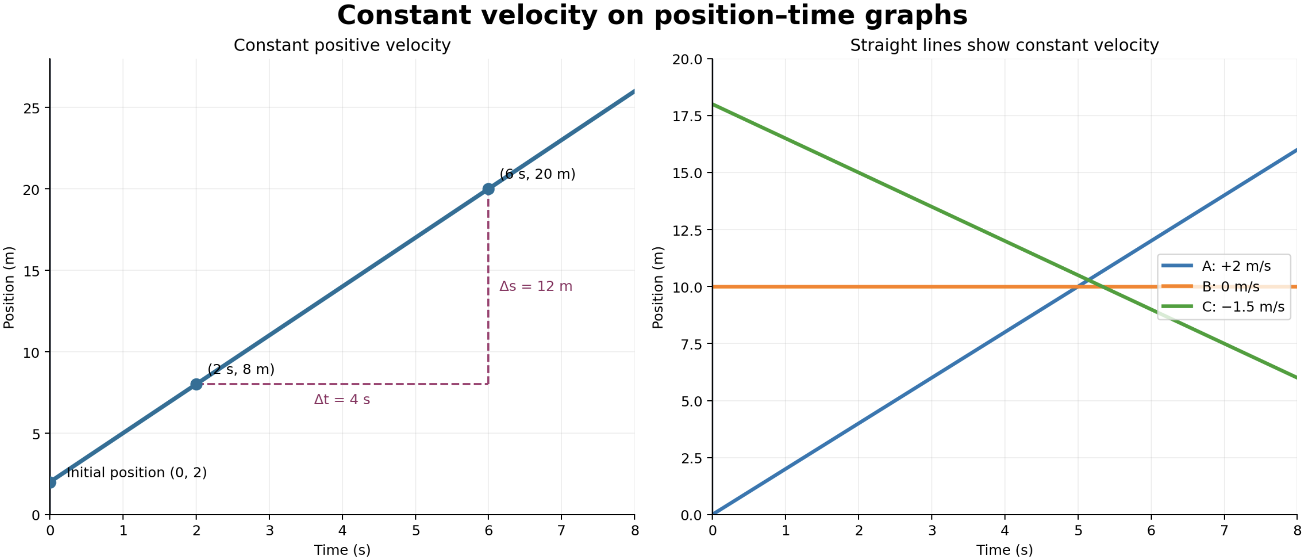
In the left graph, position changes from 8 m at 2 seconds to 20 m at 6 seconds.
The velocity is:
v = (20 − 8)/(6 − 2)
v = 12/4
v = 3 m/s
The line crosses the position axis at 2 m, so the object’s initial position is 2 m. Its equation is:
x = 2 + 3t
Interpreting the graph equation
A constant-velocity position equation has the same structure as the equation of a straight line:
x = x₀ + vt
Compare this with:
y = c + mx
In the motion equation:
- Position x is the dependent quantity.
- Time t is the independent quantity.
- Initial position x₀ is the vertical intercept.
- Velocity v is the gradient.
For example:
x = 4 + 2.5t
means:
- The object begins at position 4 m.
- It moves in the positive direction.
- Its constant velocity is 2.5 m/s.
- Its position increases by 2.5 m each second.
For:
x = 18 − 3t
the object begins at 18 m and moves in the negative direction at 3 m/s.
Constant velocity on a velocity–time graph
A constant velocity appears as a horizontal line on a velocity–time graph.
- A horizontal line above the axis represents constant positive velocity.
- A horizontal line on the axis represents rest.
- A horizontal line below the axis represents constant negative velocity.
The gradient of a horizontal line is zero, confirming that acceleration is zero.
The signed area under the velocity–time graph gives displacement.
For an object moving at +5 m/s for 8 seconds:
Δx = 5 × 8
Δx = 40 m
This is the area of a rectangle with height 5 m/s and width 8 s.
If the velocity were −5 m/s, the signed area and displacement would be −40 m.
Identifying when the equation is appropriate
The equation Δx = vΔt applies directly when velocity remains constant throughout the chosen interval.
Appropriate situations include:
- A conveyor belt moving steadily.
- A train travelling at a fixed velocity along a straight track.
- A person walking at a constant speed in one direction.
- A spacecraft coasting with approximately constant velocity.
- A vehicle during a short interval when its speed and direction do not change.
Evidence of constant velocity may include:
- A statement that velocity is constant.
- Equal displacements during equal time intervals.
- A straight line on a position–time graph.
- A horizontal line on a velocity–time graph.
- Zero acceleration throughout the interval.
When a constant-velocity equation is not appropriate
A single constant-velocity equation is not sufficient when:
- Speed increases or decreases.
- Direction changes.
- The position–time graph is curved.
- The velocity–time graph is sloped or curved.
- The acceleration is not zero.
- A journey contains stages with different velocities.
In these situations, divide the motion into suitable intervals or use an equation that accounts for acceleration.
A car journey may contain several constant-velocity stages, even if its velocity is not constant for the entire trip.
Worked example: a journey with two constant velocities
A delivery vehicle travels east at 12 m/s for 30 seconds. It then continues east at 8 m/s for 20 seconds.
The velocity is constant within each stage but changes between the stages.
First-stage displacement:
Δx₁ = 12 × 30
Δx₁ = 360 m
Second-stage displacement:
Δx₂ = 8 × 20
Δx₂ = 160 m
Total displacement:
Δx = 360 + 160
Δx = 520 m east
Total time:
Δt = 30 + 20
Δt = 50 s
Average velocity:
v_avg = 520/50
v_avg = 10.4 m/s east
The average velocity is not found by simply averaging 12 m/s and 8 m/s unless the time spent at each velocity is equal.
Worked example: motion in opposite directions
A student walks 60 m east at 2 m/s and then 20 m west at 1 m/s.
Choose east as positive.
First stage
Δx₁ = (+2)(30)
Δx₁ = +60 m
Second stage
The student travels west, so velocity is negative:
Δx₂ = (−1)(20)
Δx₂ = −20 m
Total displacement
Δx = +60 − 20
Δx = +40 m
The student finishes 40 m east of the starting point.
Total distance
Distance = 60 + 20
Distance = 80 m
Average velocity
Total time = 30 + 20 = 50 s
v_avg = 40/50
v_avg = +0.8 m/s
Average speed
Average speed = 80/50
Average speed = 1.6 m/s
This example requires two constant-velocity stages because the direction changes.
Worked example: finding when two objects meet
Two cyclists travel along the same straight path.
- Cyclist A starts at x = 0 m and travels at +5 m/s.
- Cyclist B starts at x = 30 m and travels in the same direction at +2 m/s.
Their position equations are:
xₐ = 5t
xᵦ = 30 + 2t
They meet when their positions are equal:
5t = 30 + 2t
3t = 30
t = 10 s
Their meeting position is:
x = 5(10)
x = 50 m
Cyclist A catches Cyclist B after 10 seconds at position 50 m.
A position–time graph would show two straight lines intersecting at the point (10 s, 50 m).
Relative velocity
When objects move along the same line, relative velocity describes how quickly one object’s position changes relative to the other.
For two objects A and B:
v relative = vₐ − vᵦ
In the cycling example:
v relative = 5 − 2
v relative = 3 m/s
Cyclist A closes the 30 m gap at 3 m/s:
t = 30/3
t = 10 s
If objects move towards each other, their closing speed is the sum of their speed magnitudes.
For example, two vehicles approach one another at 15 m/s and 10 m/s:
Closing speed = 15 + 10
Closing speed = 25 m/s
If they begin 200 m apart:
t = 200/25
t = 8 s
Converting units
Units must be compatible before using a motion equation.
Converting kilometres to metres
1 km = 1000 m
To convert kilometres to metres, multiply by 1000.
Converting hours to seconds
1 h = 3600 s
To convert hours to seconds, multiply by 3600.
Converting between km/h and m/s
To convert km/h to m/s:
Divide by 3.6
To convert m/s to km/h:
Multiply by 3.6
For example:
72 km/h ÷ 3.6 = 20 m/s
15 m/s × 3.6 = 54 km/h
Worked example involving unit conversion
A train moves at a constant speed of 90 km/h for 40 seconds. Calculate the distance travelled in metres.
Convert the speed:
v = 90/3.6
v = 25 m/s
Use:
d = vt
d = 25 × 40
d = 1000 m
The train travels 1000 m, or 1 km.
Applying constant velocity to light travel
Light travels through a vacuum at approximately:
c = 3.00 × 10⁸ m/s
For many basic problems, this speed is treated as constant.
Worked example
A signal travels 3.84 × 10⁸ m from Earth to the Moon. Calculate its travel time.
t = d/v
t = (3.84 × 10⁸)/(3.00 × 10⁸)
t = 1.28 s
Light takes approximately 1.28 seconds to travel from Earth to the Moon.


Constant-speed models are useful for light signals and spacecraft coasting over suitable intervals. Real motions may require more detailed models when gravity or propulsion changes the velocity significantly.
A reliable problem-solving method
Use this sequence for constant-velocity problems:
- Identify the known and unknown quantities.
- Decide whether the motion has constant speed or constant velocity.
- Choose a positive direction if direction matters.
- Convert all measurements into compatible units.
- Select the appropriate form of the equation.
- Substitute values with their signs and units.
- Calculate the answer.
- State the result with units and direction where required.
- Check whether the result is reasonable.
Checking whether an answer is reasonable
Check the units
For displacement:
(m/s) × s = m
For velocity:
m ÷ s = m/s
For time:
m ÷ (m/s) = s
Estimate the size
An object moving at 10 m/s for 5 seconds should travel about 50 m. An answer of 5000 m would suggest an error.
Check the direction
A negative displacement should agree with motion in the chosen negative direction.
Check the graph
Constant velocity should produce:
- A straight position–time graph.
- A horizontal velocity–time graph.
- A zero acceleration–time graph.
Substitute back
If an object travels 150 m at 6 m/s:
t = 150/6 = 25 s
Check:
6 × 25 = 150 m
Assumptions in constant-velocity models
Mathematical models simplify real motion. A constant-velocity model assumes:
- The object moves along a straight line.
- Its speed remains unchanged.
- Its direction remains unchanged.
- The time interval is measured accurately.
- Any brief starting or stopping stages are excluded or treated separately.
A real train may speed up, slow down and follow curved tracks. However, one steady section of its journey may still be modelled using constant velocity.
The model is useful when its assumptions are reasonable for the interval being studied.
Common misconceptions
- “Constant velocity means the object is stationary.” It can move steadily with zero acceleration.
- “Constant speed always means constant velocity.” Direction must also remain constant.
- “Distance and displacement are identical.” They are equal only in suitable one-direction motion.
- “A negative velocity means the object is slowing down.” It indicates motion in the chosen negative direction.
- “The initial position is always zero.” An object can begin anywhere relative to the origin.
- “Δx = vt applies to an entire changing-velocity journey.” Use separate stages or an acceleration model.
- “Average velocity is always the average of two velocities.” It is total displacement divided by total time.
- “A horizontal position–time graph represents constant non-zero velocity.” It represents zero velocity.
Did you know?
Constant velocity does not require zero forces. It requires zero resultant force.
For example, a car travelling steadily may have a forward driving force balanced by air resistance and friction. The forces cancel, so acceleration is zero and velocity remains constant.
Key terms
- Constant velocity: Motion with unchanged speed and direction.
- Displacement: Change in position, including direction.
- Distance: Total length of the path travelled.
- Velocity: Rate of change of displacement.
- Speed: Rate at which distance is travelled.
- Acceleration: Rate of change of velocity.
- Initial position: The object’s position at the beginning of an interval.
- Final position: The object’s position at the end of an interval.
- Time interval: The elapsed time between two events.
- Relative velocity: The velocity of one object compared with another.
- Model: A simplified mathematical description of a real situation.
Key takeaways
- Constant velocity requires constant speed and constant direction.
- An object moving at constant velocity has zero acceleration.
- Use Δx = vΔt for constant-velocity motion.
- Use x = x₀ + vΔt when the initial position is known.
- Direction can be represented using positive and negative signs.
- A straight position–time graph represents constant velocity.
- A horizontal velocity–time graph represents constant velocity.
- Divide journeys into stages when velocity changes.
- Check units, signs, assumptions and physical reasonableness.
2. Uniformly Accelerated Motion
Learning outcomes
- I can describe uniformly accelerated motion as motion with constant acceleration.
- I can identify the variables used in the equations of motion.
- I can apply the kinematic equations to uniformly accelerated motion.
- I can calculate displacement, velocity, acceleration, or time using the appropriate equation.
- I can interpret the physical meaning of solutions to kinematics problems.
What is uniformly accelerated motion?
Uniformly accelerated motion is motion in which acceleration remains constant.
Constant acceleration means that velocity changes by equal amounts during equal time intervals.
For example, if an object has an acceleration of 3 m/s², its velocity changes by 3 m/s every second:
| Time (s) | Velocity (m/s) |
|---|---|
| 0 | 2 |
| 1 | 5 |
| 2 | 8 |
| 3 | 11 |
| 4 | 14 |
The velocity increases by 3 m/s during every one-second interval. Therefore, the acceleration is constant at 3 m/s².
Uniform acceleration does not mean constant velocity. The velocity is changing, but it changes at a constant rate.
Positive and negative acceleration
The sign of acceleration describes its direction relative to a chosen positive direction.
- Positive acceleration acts in the positive direction.
- Negative acceleration acts in the negative direction.
- Zero acceleration means velocity is constant.
Negative acceleration does not always mean that an object is slowing down.
| Velocity | Acceleration | Effect on speed |
|---|---|---|
| Positive | Positive | Speed increases |
| Positive | Negative | Speed decreases |
| Negative | Positive | Speed decreases |
| Negative | Negative | Speed increases |
An object speeds up when velocity and acceleration have the same direction. It slows down when velocity and acceleration have opposite directions.
The five kinematic variables
The equations for uniformly accelerated motion use five main variables. They are often called the SUVAT variables.
| Symbol | Quantity | SI unit |
|---|---|---|
| s | Displacement | metre, m |
| u | Initial velocity | metre per second, m/s |
| v | Final velocity | metre per second, m/s |
| a | Constant acceleration | metre per second squared, m/s² |
| t | Time interval | second, s |
In some resources, displacement may be written as Δx instead of s. These symbols represent the same type of quantity: the change in position.
Be careful with u and v:
- u is the velocity at the beginning of the chosen interval.
- v is the velocity at the end of the chosen interval.
These letters do not represent directions by themselves. Direction is communicated through positive and negative signs.
The equations of uniformly accelerated motion
The standard equations are:
v = u + at
s = [(u + v)/2]t
s = ut + ½at²
v² = u² + 2as
s = vt − ½at²
Each equation assumes:
- Acceleration is constant.
- Motion is along a straight line or treated one dimension at a time.
- All values refer to the same time interval.
- A consistent positive direction is used.
These equations are not suitable for an interval in which acceleration changes.
Understanding where the equations come from
The equations are connected to the definitions of acceleration and displacement.
Velocity equation
For constant acceleration:
a = (v − u)/t
Multiply by t:
at = v − u
Rearrange:
v = u + at
This equation shows that the final velocity equals the initial velocity plus the change in velocity.
Average velocity equation
When acceleration is constant, velocity changes linearly from u to v. The average velocity is:
Average velocity = (u + v)/2
Displacement equals average velocity multiplied by time:
s = [(u + v)/2]t
This simple average applies because acceleration is constant.
Displacement equation
Substitute v = u + at into the average-velocity equation:
s = [(u + u + at)/2]t
s = [(2u + at)/2]t
Therefore:
s = ut + ½at²
The term ut represents the displacement the object would cover at its initial velocity. The term ½at² represents the additional displacement caused by acceleration.
Uniform acceleration on motion graphs
On a velocity–time graph, constant acceleration appears as a straight line because its gradient remains constant.
The gradient gives acceleration:
a = Δv/Δt
The area under the velocity–time graph gives displacement.
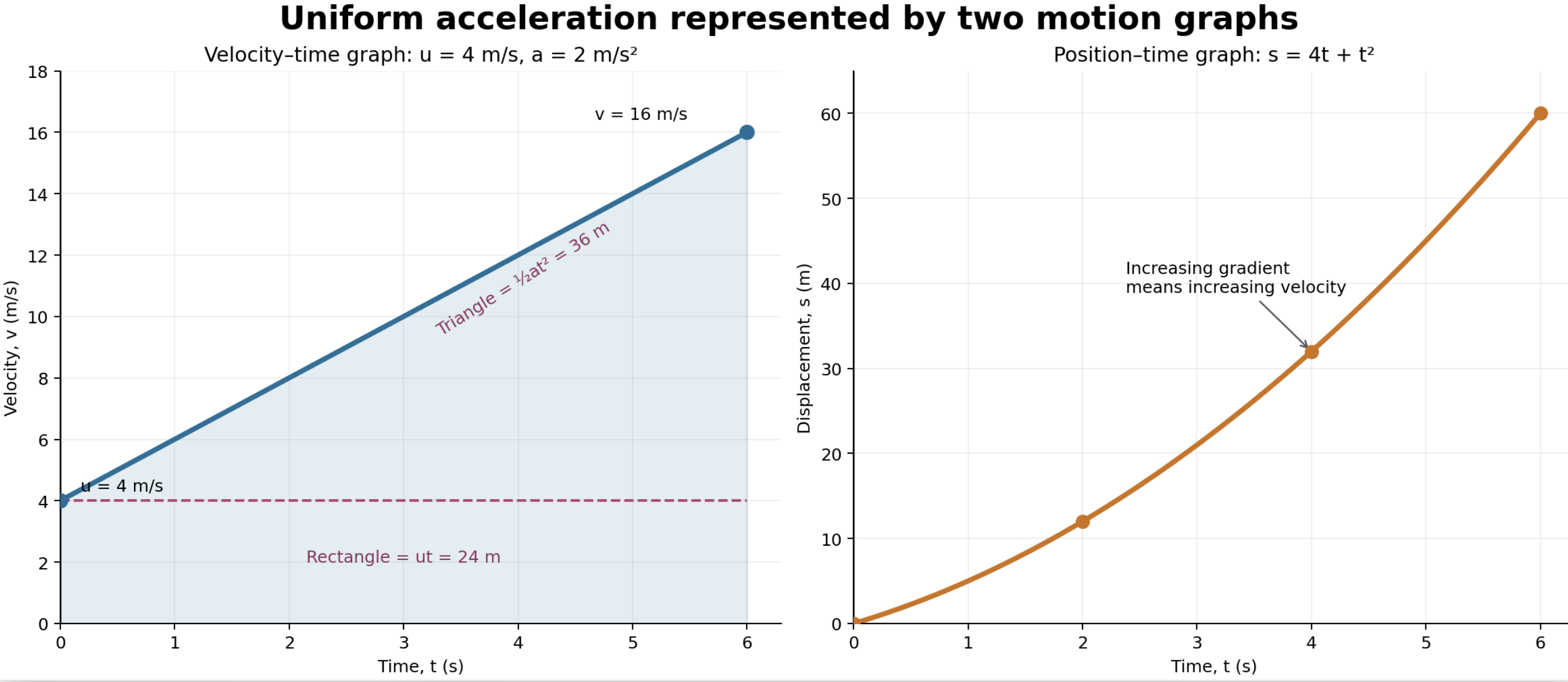
In this example:
u = 4 m/s
a = 2 m/s²
t = 6 s
The final velocity is:
v = u + at
v = 4 + 2(6)
v = 16 m/s
The displacement is the area under the velocity–time graph.
Rectangle:
ut = 4 × 6
ut = 24 m
Triangle:
½at² = ½ × 2 × 6²
½at² = 36 m
Total displacement:
s = 24 + 36
s = 60 m
The position–time graph curves upwards because its gradient, which represents velocity, continually increases.
Choosing the appropriate equation
A useful strategy is to identify the known variables and the unknown variable before selecting an equation.
| Equation | Variable absent |
|---|---|
| v = u + at | s |
| s = [(u + v)/2]t | a |
| s = ut + ½at² | v |
| v² = u² + 2as | t |
| s = vt − ½at² | u |
Choose an equation that contains:
- The quantity you need to find.
- The quantities you already know.
- As few additional unknowns as possible.
For example, if you know u, a and t and need v, use:
v = u + at
If you know u, v and a and need s, use:
v² = u² + 2as
This equation is especially useful when time is not known.
A reliable problem-solving method
Use the following method for each problem:
- Draw a simple diagram where useful.
- Choose a positive direction.
- List the known variables with signs and units.
- Identify the unknown variable.
- Select an equation containing those variables.
- Rearrange the equation if necessary.
- Substitute the values.
- Calculate and include the correct unit.
- Interpret the sign and physical meaning.
- Check whether the answer is reasonable.
Writing the variables first reduces the chance of choosing an unsuitable equation.
Worked example: finding final velocity
A car has an initial velocity of 8 m/s and accelerates uniformly at 3 m/s² for 5 seconds. Calculate its final velocity.
Known values:
u = 8 m/s
a = 3 m/s²
t = 5 s
v = ?
Choose:
v = u + at
Substitute:
v = 8 + 3(5)
v = 8 + 15
v = 23 m/s
The car’s velocity increases by 15 m/s during the five seconds, giving a final velocity of 23 m/s.


A straight test track provides a useful setting for one-dimensional acceleration problems. A real vehicle’s acceleration may vary, so the uniform model applies only over an interval where constant acceleration is a reasonable approximation.
Worked example: finding displacement
A cyclist travels at an initial velocity of 4 m/s and accelerates uniformly at 1.5 m/s² for 8 seconds. Calculate the displacement.
Known values:
u = 4 m/s
a = 1.5 m/s²
t = 8 s
s = ?
The final velocity is not required, so use:
s = ut + ½at²
Substitute:
s = 4(8) + ½(1.5)(8²)
s = 32 + 0.75(64)
s = 32 + 48
s = 80 m
The cyclist moves 80 m in the positive direction.
Worked example: finding acceleration
A train increases its velocity from 10 m/s to 22 m/s in 8 seconds. Calculate its acceleration.
Known values:
u = 10 m/s
v = 22 m/s
t = 8 s
a = ?
Use:
v = u + at
Rearrange:
a = (v − u)/t
Substitute:
a = (22 − 10)/8
a = 12/8
a = 1.5 m/s²
The train’s velocity increases by 1.5 m/s every second.
Worked example: finding time
A skateboarder accelerates uniformly from 3 m/s to 11 m/s at 2 m/s². Calculate the time taken.
Known values:
u = 3 m/s
v = 11 m/s
a = 2 m/s²
t = ?
Use:
v = u + at
Rearrange:
t = (v − u)/a
Substitute:
t = (11 − 3)/2
t = 8/2
t = 4 s
Worked example: when time is not known
A motorcycle moving at 12 m/s accelerates uniformly at 4 m/s² over a displacement of 40 m. Calculate its final velocity.
Known values:
u = 12 m/s
a = 4 m/s²
s = 40 m
v = ?
Time is not known, so use:
v² = u² + 2as
Substitute:
v² = 12² + 2(4)(40)
v² = 144 + 320
v² = 464
v = √464
v ≈ 21.5 m/s
Mathematically, taking a square root can produce positive and negative roots. In this situation, the motorcycle continues in the chosen positive direction, so the positive root is physically appropriate.
Worked example: uniform deceleration
A car travelling at 24 m/s brakes uniformly and stops in 6 seconds. Calculate its acceleration and braking displacement.
Choose the original direction of travel as positive.
Known values:
u = 24 m/s
v = 0 m/s
t = 6 s
Find the acceleration
Use:
v = u + at
Rearrange:
a = (v − u)/t
a = (0 − 24)/6
a = −4 m/s²
The negative sign shows that acceleration acts opposite to the original motion.
Find the braking displacement
Use average velocity:
s = [(u + v)/2]t
s = (24 + 0)/2
s = 12 × 6
s = 72 m
The car travels 72 m while braking.


Braking can often be approximated as uniform deceleration in introductory problems. Road conditions, tyres and braking systems cause real acceleration to vary.
Starting from rest
If an object begins from rest:
u = 0
The equations simplify.
Final velocity:
v = at
Displacement:
s = ½at²
Velocity and displacement:
v² = 2as
“Starts from rest” is important information and should immediately be recorded as u = 0.
Worked example
A trolley starts from rest and accelerates uniformly at 2.5 m/s² for 4 seconds.
Final velocity:
v = at
v = 2.5(4)
v = 10 m/s
Displacement:
s = ½at²
s = ½(2.5)(4²)
s = 1.25(16)
s = 20 m
Coming to rest
If an object stops at the end of an interval:
v = 0
“Comes to rest,” “stops,” and “reaches zero velocity” all indicate v = 0.
This does not mean that acceleration is zero during the stopping interval. A non-zero acceleration is required to change the velocity.
At the exact moment an object reaches zero velocity, it may still have non-zero acceleration.
Free fall as uniform acceleration
Near Earth’s surface, an object in free fall has an approximately constant downward acceleration:
g ≈ 9.8 m/s²
For simpler calculations, g may be rounded to 10 m/s².
An object is in free fall when gravity is the only significant force acting on it. Air resistance is ignored.


In a stroboscopic image, the increasing gaps between successive positions of a falling object show that its speed is increasing.
Choosing signs in vertical motion
If upward is chosen as positive:
a = −9.8 m/s²
If downward is chosen as positive:
a = +9.8 m/s²
Either choice works if it is used consistently.
Worked example: dropping an object
A stone is dropped from rest and falls for 3 seconds. Ignore air resistance and use g = 9.8 m/s². Choose downward as positive.
Known values:
u = 0 m/s
a = +9.8 m/s²
t = 3 s
Final velocity
v = u + at
v = 0 + 9.8(3)
v = 29.4 m/s downward
Displacement
s = ut + ½at²
s = 0 + ½(9.8)(3²)
s = 4.9(9)
s = 44.1 m downward
The velocity and displacement are both positive because downward was selected as the positive direction.
Worked example: throwing an object upwards
A ball is thrown vertically upwards at 19.6 m/s. Ignore air resistance. Find the time taken to reach its highest point.
Choose upward as positive.
Known values:
u = +19.6 m/s
v = 0 m/s at the highest point
a = −9.8 m/s²
t = ?
Use:
v = u + at
0 = 19.6 − 9.8t
9.8t = 19.6
t = 2.0 s
The ball takes 2.0 seconds to reach its highest point.
At that point:
- Its instantaneous velocity is zero.
- Its acceleration is still −9.8 m/s².
- It is about to begin moving downwards.
Finding maximum height
Using the same upward-thrown ball:
u = 19.6 m/s
v = 0 m/s
a = −9.8 m/s²
Time is not required, so use:
v² = u² + 2as
0² = 19.6² + 2(−9.8)s
0 = 384.16 − 19.6s
19.6s = 384.16
s = 19.6 m
The ball rises 19.6 m above its release point.
Problems with two possible times
Some displacement problems produce a quadratic equation and two mathematical solutions.
Worked example
A ball is thrown upwards from ground level at 20 m/s. Its height is modelled using g = 10 m/s²:
s = ut + ½at²
s = 20t − 5t²
Find when the ball is 15 m above the ground:
15 = 20t − 5t²
Rearrange:
5t² − 20t + 15 = 0
Divide by 5:
t² − 4t + 3 = 0
Factorize:
(t − 1)(t − 3) = 0
Therefore:
t = 1 s or t = 3 s
Both solutions are physically meaningful:
- At 1 second, the ball passes 15 m while rising.
- At 3 seconds, it passes 15 m again while falling.
A complete answer must interpret both solutions.
Interpreting negative time solutions
A quadratic equation may also produce a negative time.
Suppose a problem asks what happens after t = 0. A solution such as t = −2 s refers to a time before the chosen starting moment and is normally rejected for that context.
Do not reject a solution simply because it is negative. First identify what the sign represents:
- Negative time may lie outside the modelled interval.
- Negative velocity may indicate direction.
- Negative displacement may indicate a final position in the negative direction.
- Negative acceleration may indicate acceleration in the negative direction.
Interpret each sign using the problem’s coordinate system.
Multi-stage motion
A single kinematic equation applies only while acceleration is constant.
If acceleration changes, divide the journey into stages.
For example, a car may:
- Accelerate at 2 m/s² for 5 seconds.
- Travel at constant velocity for 10 seconds.
- Decelerate at −4 m/s² until stopping.
For each stage:
- The final velocity of one stage becomes the initial velocity of the next.
- Calculate the displacement separately.
- Add displacements algebraically to find total displacement.
- Add distance magnitudes when total distance is required.
- Add the stage times to find total time.
Do not apply one constant-acceleration equation across the whole journey unless acceleration is constant throughout it.
Dimensional checks
Units can help verify an equation.
For:
s = ut + ½at²
The term ut has units:
(m/s)(s) = m
The term at² has units:
(m/s²)(s²) = m
Both terms have units of displacement, so they can be added.
For:
v² = u² + 2as
Each term has units:
m²/s²
A proposed equation such as v = u + as would be invalid because u and as have different units.
Checking whether an answer is reasonable
Check the direction
Does the sign match the direction described in the problem?
Check the size
An object accelerating at 2 m/s² for 3 seconds changes velocity by 6 m/s. A calculated change of 60 m/s probably contains an error.
Check the limiting case
If a = 0:
v = u + at becomes v = u
s = ut + ½at² becomes s = ut
The equations reduce correctly to constant-velocity motion.
Substitute into another equation
If enough information is available, verify the result using a second kinematic equation.
Compare with a graph
Uniform acceleration should produce:
- A straight velocity–time graph.
- A horizontal acceleration–time graph.
- A curved position–time graph.
Common misconceptions
- “Uniform acceleration means constant velocity.” It means velocity changes at a constant rate.
- “Negative acceleration always means slowing down.” Compare the directions of velocity and acceleration.
- “The final velocity is always greater than the initial velocity.” It may be smaller or have the opposite sign.
- “An object at rest has no acceleration.” It may have zero velocity at one instant while still accelerating.
- “Every answer from a quadratic equation is physically meaningful.” Check the time interval and context.
- “The equations work for any changing motion.” They require constant acceleration.
- “Displacement and distance are interchangeable.” Displacement includes direction and can be negative.
- “A negative result must be wrong.” It often communicates direction.
Did you know?
The equation:
s = ut + ½at²
shows that displacement depends on the square of time when acceleration is constant.
For an object starting from rest, doubling the time makes the displacement four times as large:
s = ½a(2t)²
s = 4(½at²)
This is why the gaps between successive positions of a freely falling object become increasingly large.
Key terms
- Uniformly accelerated motion: Motion with constant acceleration.
- Initial velocity: Velocity at the beginning of an interval, represented by u.
- Final velocity: Velocity at the end of an interval, represented by v.
- Displacement: Change in position, represented by s or Δx.
- Acceleration: Rate of change of velocity, represented by a.
- Time interval: Elapsed time during the motion, represented by t.
- SUVAT equations: Equations connecting displacement, initial velocity, final velocity, acceleration and time.
- Free fall: Motion in which gravity is the only significant force.
- Average velocity: Total displacement divided by total time.
- Sign convention: A consistent choice of positive and negative directions.
- Physical solution: A mathematical answer that fits the conditions of the situation.
Key takeaways
- Uniform acceleration means acceleration remains constant.
- List the SUVAT variables before selecting an equation.
- Choose the equation that contains the known values and required unknown.
- Use positive and negative signs consistently to represent direction.
- Uniform acceleration produces a straight velocity–time graph.
- The area under a velocity–time graph gives displacement.
- Free fall is approximately uniform acceleration when air resistance is ignored.
- Divide changing motion into stages when acceleration is not constant.
- Interpret every solution using its sign, units and physical context.
3. Solving Kinematics Problems
Learning outcomes
- I can identify known and unknown variables in a motion problem.
- I can organize information using diagrams, tables, or variable lists.
- I can select and apply appropriate equations to solve problems.
- I can show complete and logical solutions using correct units.
- I can evaluate whether an answer is reasonable.
What is a kinematics problem?
Kinematics is the study of motion without focusing on the forces that cause it.
A kinematics problem may ask you to determine:
- An object’s displacement.
- Its initial or final velocity.
- Its acceleration.
- The time taken.
- Where or when two objects meet.
- The distance travelled during a journey.
- The maximum height of a moving object.
Solving these problems requires more than inserting numbers into an equation. You must first understand the motion, organize the information and choose a mathematical model that fits the situation.
A reliable problem-solving method
A complete solution can be organized into five stages:
- Represent the motion.
- Organize the information.
- Select an appropriate equation.
- Solve carefully.
- Evaluate the result.
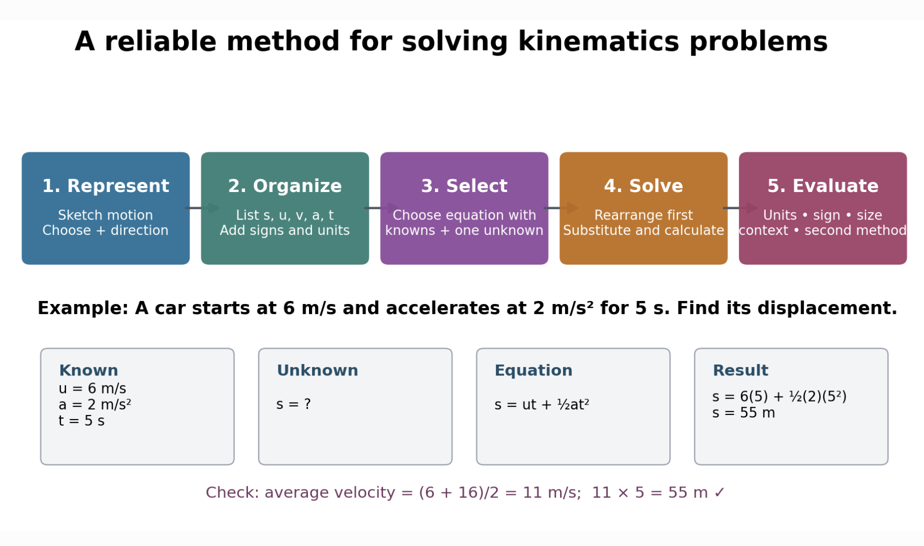
This method makes each decision visible. It also makes errors easier to find and correct.
Reading a motion problem carefully
Begin by identifying words and phrases that communicate mathematical information.
| Phrase in the problem | Mathematical meaning |
|---|---|
| Starts from rest | u = 0 |
| Comes to rest or stops | v = 0 |
| Constant velocity | a = 0 |
| Uniform acceleration | a is constant |
| Falls freely | a = g downward |
| Returns to its starting point | Total displacement = 0 |
| Moves east, right or upwards | Often chosen as positive |
| Moves west, left or downwards | Often represented as negative |
| Maximum height | Vertical velocity is momentarily zero |
| Ignore air resistance | Gravity is the only significant acceleration |
Do not assume information that the problem does not provide. For example, “a car moves at 20 m/s” does not mean it started from rest.
Identifying the variables
For uniformly accelerated motion, organize information using the five SUVAT variables.
| Symbol | Quantity | SI unit |
|---|---|---|
| s | Displacement | m |
| u | Initial velocity | m/s |
| v | Final velocity | m/s |
| a | Acceleration | m/s² |
| t | Time | s |
For constant-velocity motion, the main relationship is:
s = vt
or, when an initial position is included:
x = x₀ + vt
Before choosing an equation, write down each known value and the required unknown.
For example:
A car starts at 6 m/s and accelerates at 2 m/s² for 5 seconds. Find its displacement.
Known:
u = 6 m/s
a = 2 m/s²
t = 5 s
Unknown:
s = ?
The unused variable is v, so an equation that does not contain v is convenient.
Drawing a motion diagram
A simple diagram can clarify:
- The direction of motion.
- The chosen positive direction.
- The starting and finishing positions.
- Whether the object reverses direction.
- Whether several objects are involved.
- Whether the journey contains multiple stages.
A diagram does not need to be artistic. A line, arrows and labels are often sufficient.
For example:
Start: x = 0 m →→→ Finish: x = 80 m
Positive direction: →
A vertical-motion diagram might show:
- The release point.
- The highest point.
- The ground.
- The upward positive direction.
- The downward acceleration due to gravity.


A photograph or sequence can help visualize the situation, but the mathematical diagram should isolate only the positions, directions and quantities needed for the calculation.
Choosing a positive direction
Velocity, acceleration and displacement are vectors. Their signs depend on the chosen coordinate system.
For horizontal motion, you might choose:
- Right or east as positive.
- Left or west as negative.
For vertical motion, you might choose:
- Upwards as positive and gravity negative.
- Downwards as positive and gravity positive.
Either choice works if it is used consistently.
Suppose east is positive:
- A velocity of 12 m/s east is +12 m/s.
- A displacement of 30 m west is −30 m.
- An acceleration acting west is negative.
The sign belongs with the numerical value when it is listed. Do not wait until the end to decide which values should be negative.
Selecting an equation
The equations of uniformly accelerated motion are:
v = u + at
s = [(u + v)/2]t
s = ut + ½at²
v² = u² + 2as
s = vt − ½at²
Each equation omits one SUVAT variable.
| Equation | Variable not included |
|---|---|
| v = u + at | s |
| s = [(u + v)/2]t | a |
| s = ut + ½at² | v |
| v² = u² + 2as | t |
| s = vt − ½at² | u |
Choose the equation containing the known quantities and the one unknown you need.
Do not select an equation simply because it looks familiar. Match its variables to the information in the problem.
Worked example: finding displacement
A car has an initial velocity of 6 m/s and accelerates uniformly at 2 m/s² for 5 seconds. Calculate its displacement.
Known:
u = 6 m/s
a = 2 m/s²
t = 5 s
s = ?
The final velocity is not known or required. Choose:
s = ut + ½at²
Substitute:
s = 6(5) + ½(2)(5²)
s = 30 + 25
s = 55 m
Checking with a second method
First calculate the final velocity:
v = u + at
v = 6 + 2(5)
v = 16 m/s
Because acceleration is constant:
Average velocity = (u + v)/2
Average velocity = (6 + 16)/2
Average velocity = 11 m/s
Therefore:
s = 11 × 5
s = 55 m
Both methods produce the same answer.
Rearranging before substituting
When possible, rearrange an equation symbolically before inserting numbers. This keeps the logic clear and reduces calculator errors.
Worked example
A cyclist increases velocity from 4 m/s to 16 m/s over a displacement of 60 m. Calculate the constant acceleration.
Known:
u = 4 m/s
v = 16 m/s
s = 60 m
a = ?
Time is not given, so choose:
v² = u² + 2as
Rearrange for a:
v² − u² = 2as
a = (v² − u²)/(2s)
Substitute:
a = (16² − 4²)/(2 × 60)
a = (256 − 16)/120
a = 240/120
a = 2 m/s²
Showing a complete solution
A complete kinematics solution should include:
- The known variables.
- The unknown variable.
- A direction convention where needed.
- The equation used.
- Any rearrangement.
- Substitution with values.
- The calculated result.
- Correct units.
- Direction or physical interpretation where appropriate.
Writing only a calculator result makes it difficult to check the reasoning.
A clear solution might look like this:
Known: u = 4 m/s, v = 16 m/s, s = 60 m
Required: a
Equation: v² = u² + 2as
Rearrange: a = (v² − u²)/(2s)
Substitute: a = (16² − 4²)/(2 × 60)
Result: a = 2 m/s²
Worked example: uniform deceleration
A train moving at 30 m/s slows uniformly to 12 m/s in 9 seconds. Calculate its acceleration and displacement.
Choose the original direction of travel as positive.
Known:
u = 30 m/s
v = 12 m/s
t = 9 s
Calculate acceleration
Use:
v = u + at
Rearrange:
a = (v − u)/t
Substitute:
a = (12 − 30)/9
a = −18/9
a = −2 m/s²
The negative sign shows that the acceleration acts opposite to the train’s positive velocity.
Calculate displacement
Use:
s = [(u + v)/2]t
s = (30 + 12)/2
s = 21 × 9
s = 189 m
The train continues moving forwards while slowing down.


A train’s real acceleration may change during braking. A constant-acceleration model approximates the motion over an interval in which the velocity decreases at a steady rate.
Worked example: starting from rest
A runner starts from rest and accelerates uniformly at 1.2 m/s² for 6 seconds. Calculate the final velocity and displacement.
“Starts from rest” means:
u = 0 m/s
Final velocity
v = u + at
v = 0 + 1.2(6)
v = 7.2 m/s
Displacement
s = ut + ½at²
s = 0 + ½(1.2)(6²)
s = 0.6(36)
s = 21.6 m
A common error is to use the final velocity for the entire six seconds:
7.2 × 6 = 43.2 m
This is incorrect because the runner did not travel at 7.2 m/s for the whole interval. The runner began at rest and gradually reached that velocity.
Worked example: finding time
A motorcycle accelerates uniformly from 8 m/s to 24 m/s at 4 m/s². Calculate the time taken.
Known:
u = 8 m/s
v = 24 m/s
a = 4 m/s²
t = ?
Use:
v = u + at
Rearrange:
t = (v − u)/a
Substitute:
t = (24 − 8)/4
t = 16/4
t = 4 s
Check:
The motorcycle gains 4 m/s each second. A gain of 16 m/s should therefore take four seconds.
Problems involving constant velocity
Not every kinematics problem requires the uniformly accelerated motion equations.
If velocity is constant:
a = 0
Use:
s = vt
Worked example
A boat travels north at a constant velocity of 7.5 m/s for 40 seconds. Find its displacement.
s = vt
s = 7.5 × 40
s = 300 m north
Using s = ut + ½at² would also work if u = 7.5 m/s and a = 0, but the simpler constant-velocity equation is more efficient.
Problems involving free fall
Near Earth’s surface, free-falling objects have an approximately constant downward acceleration:
g = 9.8 m/s²
Air resistance is ignored in basic free-fall problems.
Worked example: dropping an object
A ball is dropped from a bridge and falls for 2.5 seconds. Calculate its downward displacement. Ignore air resistance.
Choose downward as positive.
Known:
u = 0 m/s
a = +9.8 m/s²
t = 2.5 s
s = ?
Use:
s = ut + ½at²
s = 0 + ½(9.8)(2.5²)
s = 4.9(6.25)
s = 30.6 m downward
The ball falls approximately 30.6 m.
Worked example: throwing an object upwards
A ball is thrown vertically upwards at 24 m/s. Calculate the time required to reach its highest point. Ignore air resistance.
Choose upwards as positive:
u = +24 m/s
v = 0 m/s
a = −9.8 m/s²
t = ?
At maximum height, the ball’s velocity is momentarily zero.
Use:
v = u + at
0 = 24 − 9.8t
9.8t = 24
t = 24/9.8
t ≈ 2.45 s
The ball reaches its highest point after approximately 2.45 seconds.
Its acceleration remains −9.8 m/s² at the highest point.
Problems with more than one solution
A quadratic equation may produce two possible times.
For example, a ball is thrown upwards from the ground with:
s = 20t − 5t²
Find when it is 15 m above the ground:
15 = 20t − 5t²
Rearrange:
5t² − 20t + 15 = 0
Divide by 5:
t² − 4t + 3 = 0
Factorize:
(t − 1)(t − 3) = 0
Therefore:
t = 1 s or t = 3 s
Both answers are reasonable:
- The ball passes 15 m while rising at 1 second.
- It passes 15 m again while falling at 3 seconds.
A complete solution interprets why two answers occur.
Problems involving two objects
When two objects meet, their positions are equal at the same time.
Worked example
Two cyclists move along the same straight road.
- Cyclist A starts at x = 0 m and moves at 6 m/s.
- Cyclist B starts 40 m ahead and moves in the same direction at 4 m/s.
Write their position equations:
xₐ = 6t
xᵦ = 40 + 4t
At the meeting point:
xₐ = xᵦ
Therefore:
6t = 40 + 4t
2t = 40
t = 20 s
Find the meeting position:
x = 6(20)
x = 120 m
Cyclist A catches Cyclist B after 20 seconds, 120 m from A’s starting point.
Multi-stage motion problems
Many real journeys contain several stages.
A car might:
- Accelerate from rest.
- Travel at constant velocity.
- Decelerate to a stop.
Treat each stage separately because the motion conditions change.
For each stage:
- List a new set of variables.
- Use the final velocity of one stage as the initial velocity of the next.
- Calculate the stage displacement.
- Add signed displacements for total displacement.
- Add distance magnitudes for total distance.
- Add all stage times for total time.
Worked example
A car:
- Accelerates from rest at 2 m/s² for 5 seconds.
- Travels at constant velocity for 8 seconds.
- Decelerates uniformly to rest in 4 seconds.
Stage 1: accelerating
u = 0 m/s
a = 2 m/s²
t = 5 s
Final velocity:
v = u + at
v = 0 + 2(5)
v = 10 m/s
Displacement:
s₁ = ut + ½at²
s₁ = 0 + ½(2)(5²)
s₁ = 25 m
Stage 2: constant velocity
v = 10 m/s
t = 8 s
s₂ = vt
s₂ = 10(8)
s₂ = 80 m
Stage 3: decelerating
u = 10 m/s
v = 0 m/s
t = 4 s
s₃ = [(u + v)/2]t
s₃ = (10 + 0)/2
s₃ = 20 m
Entire journey
Total displacement:
s = 25 + 80 + 20
s = 125 m
Total time:
t = 5 + 8 + 4
t = 17 s
Average velocity:
v_avg = 125/17
v_avg ≈ 7.35 m/s
Using graphs to check a solution
Motion graphs provide an independent way to check calculations.
Position–time graph
- Gradient gives velocity.
- A straight line represents constant velocity.
- A curve represents changing velocity.
- A horizontal tangent represents zero instantaneous velocity.
Velocity–time graph
- Vertical coordinate gives velocity.
- Gradient gives acceleration.
- Signed area gives displacement.
- A horizontal line represents zero acceleration.
Acceleration–time graph
- Vertical coordinate gives acceleration.
- Signed area gives change in velocity.
- A horizontal line represents constant acceleration.
For the multi-stage car journey, a velocity–time graph would rise from 0 to 10 m/s, remain horizontal, and then fall to zero. Its total area would be 125 m.
Converting units before calculating
Measurements must use compatible units.
Useful conversions include:
1 km = 1000 m
1 h = 3600 s
1 m/s = 3.6 km/h
To convert km/h to m/s, divide by 3.6.
To convert m/s to km/h, multiply by 3.6.
Worked example
A car travelling at 72 km/h accelerates uniformly to 30 m/s in 5 seconds. Find its acceleration.
Convert the initial velocity:
u = 72/3.6
u = 20 m/s
Now use:
a = (v − u)/t
a = (30 − 20)/5
a = 2 m/s²
Using 72 and 30 directly would mix incompatible units.
Significant figures and precision
A final answer should usually reflect the precision of the data.
For example, if a distance is given as 25 m and a time as 3.2 s:
v = 25/3.2
v = 7.8125 m/s
A suitable reported answer is:
v ≈ 7.8 m/s
Do not round intermediate values too early. Keep extra calculator digits during the calculation and round the final result.
When a problem states that g = 9.8 m/s², answers generally should not imply greater precision than that value supports.
Evaluating whether an answer is reasonable
Check the units
Each calculated quantity requires an appropriate unit:
- Displacement: m.
- Velocity: m/s.
- Acceleration: m/s².
- Time: s.
For example, using s = ut + ½at²:
ut has units (m/s)(s) = m
at² has units (m/s²)(s²) = m
Both terms have displacement units.
Check the sign
A negative answer may describe direction rather than an error.
Ask:
- Which direction was chosen as positive?
- Does the sign match the motion?
- Did the object reverse direction?
- Does the question ask for a vector or a magnitude?
Check the size
Estimate before or after calculating.
A person walking for 10 seconds at about 1.5 m/s should travel roughly 15 m. An answer of 1500 m would be unreasonable.
Check against limiting cases
If acceleration is zero, the accelerated-motion equations should reduce to constant-velocity relationships.
If time is zero:
- Displacement should be zero.
- Final velocity should equal initial velocity.
Use a second method
Possible checks include:
- Using a different kinematic equation.
- Finding the area under a velocity–time graph.
- Substituting the result back into the original equation.
- Comparing it with a simple estimate.
Check the physical context
Ask whether the answer describes something possible within the model.
For example:
- A negative time may lie outside the interval being studied.
- A vehicle’s calculated speed might be unrealistically high.
- A height below ground may be outside the intended model.
- Two mathematical solutions may describe the upward and downward parts of a flight.
Diagnosing common errors
Using the wrong initial velocity
The initial velocity belongs to the beginning of the chosen interval. In a multi-stage problem, it may not be the velocity at the start of the entire journey.
Confusing final velocity with average velocity
For constant acceleration:
Average velocity = (u + v)/2
The final velocity should not be multiplied by the entire time unless velocity was constant at that value.
Ignoring direction
Substituting every value as positive can produce an incorrect result in braking, vertical-motion and reversal problems.
Mixing distance and displacement
Distance is the total path length. Displacement depends only on initial and final positions.
Mixing units
Kilometres, metres, hours and seconds must be converted into a compatible system before substitution.
Applying SUVAT across changing acceleration
If acceleration changes between stages, solve each constant-acceleration interval separately.
Rounding too early
Premature rounding can noticeably change a final answer, especially in multi-step calculations.
Did you know?
A good diagram can prevent errors before any algebra begins.
Representing the origin, positive direction and starting position helps determine the correct signs. In multi-object problems, separate position equations make it clear that the objects meet when their positions become equal.
Professional scientists and engineers use diagrams and variable definitions for the same reason: they make the model and assumptions visible.
Key terms
- Kinematics: The study of motion without considering its causes.
- Known variable: A quantity whose value is provided or can be inferred.
- Unknown variable: The quantity that must be calculated.
- SUVAT variables: Displacement, initial velocity, final velocity, acceleration and time.
- Sign convention: A consistent choice of positive and negative directions.
- Motion diagram: A simplified representation of positions, directions and motion.
- Uniform acceleration: Acceleration that remains constant.
- Free fall: Motion under the influence of gravity alone.
- Multi-stage motion: A journey divided into intervals with different motion conditions.
- Physical solution: A mathematical result that fits the stated situation.
- Dimensional check: A comparison of units used to test whether an equation or answer is consistent.
- Reasonableness check: An evaluation of whether an answer’s sign, size, units and meaning are plausible.
Key takeaways
- Read the problem carefully and translate words into variables.
- Sketch the motion and choose a positive direction.
- List known and unknown quantities with signs and units.
- Select an equation containing the known variables and required unknown.
- Rearrange before substituting when practical.
- Show the equation, substitution, calculation, unit and interpretation.
- Treat multi-stage journeys one interval at a time.
- Interpret multiple or negative solutions using the physical context.
- Check answers using units, estimates, graphs or a second method.
4. Choosing the Correct Equation
Learning outcomes
- I can identify which kinematic equation is most appropriate for a given situation.
- I can determine which variables are available and which are missing.
- I can distinguish between constant velocity and constant acceleration situations.
- I can solve problems efficiently using equation selection strategies.
- I can explain why a particular equation is suitable for a problem.
Why equation selection matters
Kinematics provides several equations for describing motion. Choosing an appropriate equation is often the most important part of solving a problem.
A suitable equation should:
- Match the type of motion being described.
- Contain the quantity you need to calculate.
- Contain the values already provided.
- Avoid introducing unnecessary unknowns.
- Be valid under the conditions of the problem.
Before calculating anything, identify the motion model and organize the available information.
Begin with the motion model
The first decision is whether the object has constant velocity or constant acceleration.
Constant velocity
Constant velocity means:
- Speed remains constant.
- Direction remains constant.
- Acceleration is zero.
- Equal displacements occur in equal time intervals.
Use:
s = vt
or, when the initial position is included:
x = x₀ + vt
Constant acceleration
Uniform acceleration means:
- Acceleration remains constant.
- Velocity changes by equal amounts in equal time intervals.
- A velocity–time graph is a straight sloping line.
- The SUVAT equations can be used.
The main equations are:
v = u + at
s = ½(u + v)t
s = ut + ½at²
v² = u² + 2as
s = vt − ½at²
If acceleration changes during the interval, these equations cannot be applied to the entire motion as one stage.
Equation-selection guide
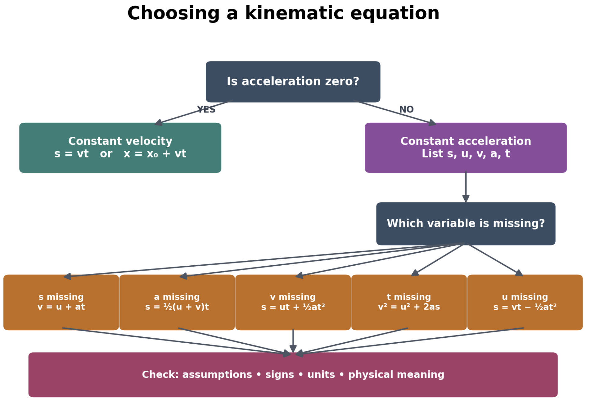
First decide whether acceleration is zero. For uniformly accelerated motion, list the five SUVAT variables and identify the variable that is absent from the problem.


5. Real-World Applications
Learning outcomes
- I can apply kinematic equations to real-world situations.
- I can analyze motion in transportation, sports, and engineering contexts.
- I can interpret motion data using equations and graphs.
- I can model physical situations using the equations of motion.
- I can explain how kinematics is used to solve practical problems.
What is a kinematic model?
A kinematic model is a mathematical description of an object’s motion. It connects quantities such as:
- Position and displacement.
- Distance travelled.
- Speed and velocity.
- Acceleration.
- Time.
Kinematic models allow us to predict where an object will be, how fast it will move and how long a motion will take.
They are used in:
- Vehicle design and road safety.
- Sports training and performance analysis.
- Roller-coaster and elevator design.
- Robotics and automated manufacturing.
- Aircraft and spacecraft navigation.
- Accident reconstruction.
- Motion sensors and tracking systems.
A model is a simplified representation of reality. Its usefulness depends on whether its assumptions are reasonable.
Selecting a motion model
Before using an equation, decide how the object is moving.
Constant velocity
Use a constant-velocity model when speed and direction remain unchanged:
s = vt
or:
x = x₀ + vt
Uniform acceleration
Use the equations of motion when acceleration remains constant:
v = u + at
s = ½(u + v)t
s = ut + ½at²
v² = u² + 2as
s = vt − ½at²
Changing acceleration
If acceleration varies significantly, a single constant-acceleration equation may not represent the entire motion.
Possible approaches include:
- Dividing the motion into shorter stages.
- Interpreting experimental graphs.
- Estimating areas and gradients.
- Using calculus or computer simulations.
- Collecting additional motion data.
From reality to a mathematical model
A practical kinematics problem can be organized into the following sequence:
- Identify the object and the interval of motion.
- Choose an origin and positive direction.
- Decide whether velocity or acceleration is constant.
- Identify the known and unknown quantities.
- Select an appropriate equation or graph method.
- Calculate the required quantity.
- Interpret the result in context.
- Evaluate the model’s assumptions and limitations.
For example, a braking car might be simplified as an object moving in a straight line with constant negative acceleration. This model ignores small changes in braking force and road conditions but can still provide a useful estimate.
Transportation: reaction and braking distances
A vehicle does not stop immediately when a driver notices a hazard.
Total stopping distance has two parts:
Total stopping distance = thinking distance + braking distance
Thinking distance
Thinking distance is the distance travelled during the driver’s reaction time.
If the vehicle travels at constant velocity during this brief interval:
Thinking distance = initial speed × reaction time
dₜ = utᵣ
Thinking distance increases directly with speed when reaction time remains constant.
Braking distance
After the brakes are applied, the vehicle decelerates.
For a simplified constant-deceleration model:
v² = u² + 2as
When the vehicle stops, v = 0. If d represents the positive magnitude of deceleration:
0 = u² − 2ds
Therefore:
Braking distance = u²/(2d)
Braking distance depends on the square of the initial speed.
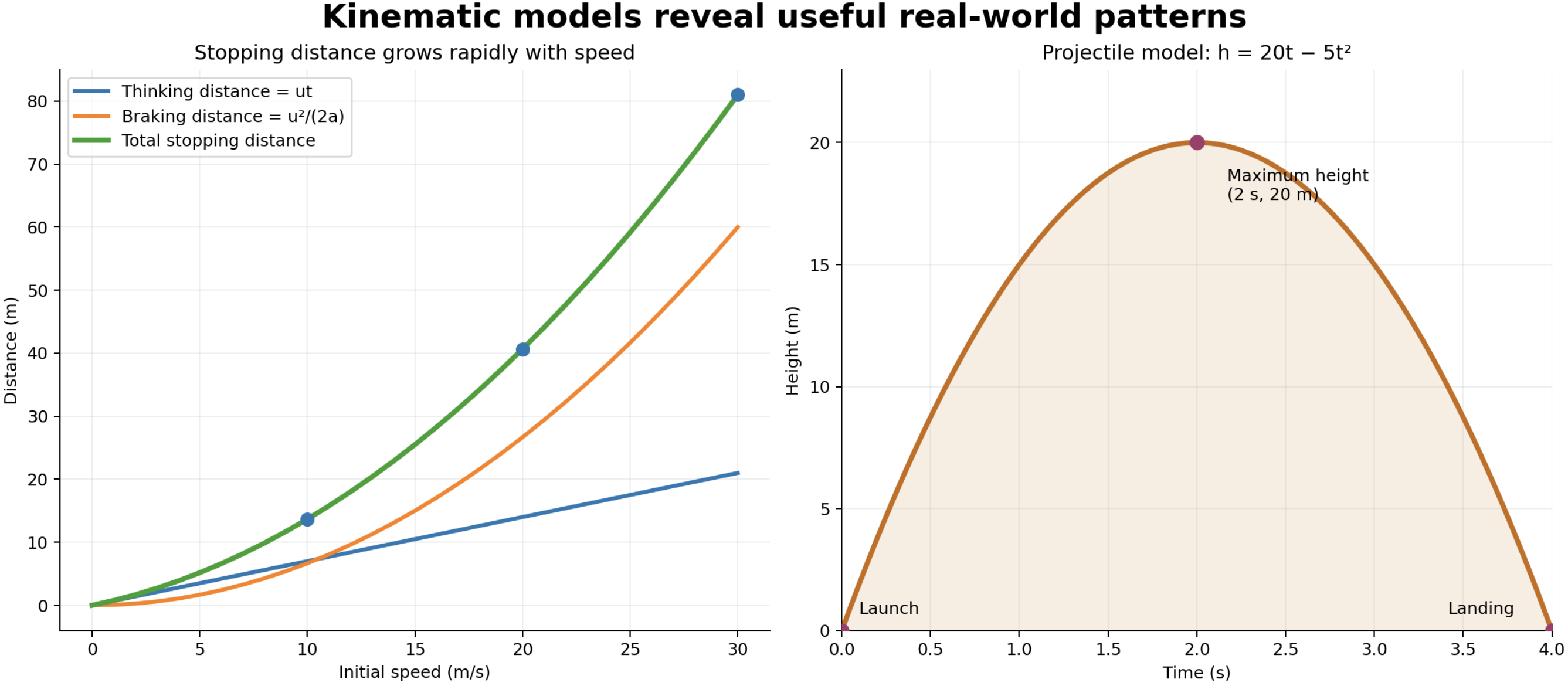
In the stopping model, reaction time is 0.7 s and the braking deceleration has magnitude 7.5 m/s². Thinking distance grows linearly with speed, while braking distance grows quadratically.
Worked example: vehicle stopping distance
A car travels at 20 m/s. The driver’s reaction time is 0.7 s, and the car then brakes uniformly with a deceleration magnitude of 7.5 m/s².
Thinking distance
dₜ = utᵣ
dₜ = 20(0.7)
dₜ = 14 m
Braking distance
Use:
v² = u² + 2as
Choose the direction of travel as positive:
u = 20 m/s
v = 0 m/s
a = −7.5 m/s²
Substitute:
0² = 20² + 2(−7.5)s
0 = 400 − 15s
15s = 400
s ≈ 26.7 m
Total stopping distance
Total distance = 14 + 26.7
Total distance ≈ 40.7 m
The car travels approximately 41 m between the driver seeing the hazard and the vehicle stopping.
Why higher speed greatly increases stopping distance
Suppose braking conditions remain unchanged.
At 10 m/s:
Braking distance = 10²/(2 × 7.5)
Braking distance ≈ 6.7 m
At 20 m/s:
Braking distance = 20²/(2 × 7.5)
Braking distance ≈ 26.7 m
Doubling the initial speed increases the braking distance by a factor of four.
This occurs because:
Braking distance ∝ speed²
The total stopping distance does not increase by exactly four because thinking distance depends directly on speed rather than speed squared.


Real braking distance depends on tyre condition, road surface, weather, brakes, vehicle mass distribution and driver response. The equation gives a model based on the stated acceleration.
Interpreting braking data from a velocity–time graph
A velocity–time graph can show a vehicle’s complete stopping process.
- A horizontal section represents the reaction interval.
- A downward-sloping section represents braking.
- The gradient during braking gives acceleration.
- The complete area under the graph gives stopping distance.
Suppose a car remains at 18 m/s for 0.8 s and then slows uniformly to rest in 3.0 s.
Thinking distance:
d = 18(0.8)
d = 14.4 m
Braking distance:
d = ½(3.0)(18)
d = 27 m
Total stopping distance:
d = 14.4 + 27
d = 41.4 m
The graphical and equation-based methods describe the same motion.
Transportation: journey planning
Constant-velocity equations can estimate travel time over a steady section of a journey.
Worked example
A train travels 36 km at a constant speed of 90 km/h. Calculate the travel time.
Use:
t = d/v
t = 36/90
t = 0.4 h
Convert to minutes:
0.4 × 60 = 24 minutes
This model assumes the train maintains 90 km/h throughout the complete 36 km. If it accelerates after leaving a station and decelerates before arriving, the actual time will be longer.


Timetables and transport simulations divide journeys into stages that include acceleration, cruising, speed restrictions and braking.
Sports: sprint acceleration
Athletes use kinematic data to study starts, acceleration and maximum speed.
A sprinter does not immediately reach top speed. The athlete accelerates strongly after leaving the starting blocks and then approaches maximum speed.
Worked example
A sprinter starts from rest and reaches 9.0 m/s after accelerating uniformly for 3.0 seconds.
Calculate the acceleration:
a = (v − u)/t
a = (9.0 − 0)/3.0
a = 3.0 m/s²
Calculate the displacement:
s = ½(u + v)t
s = ½(0 + 9.0)(3.0)
s = 13.5 m
Under this simplified model, the runner covers 13.5 m during the acceleration stage.
Real sprint acceleration is not perfectly constant. The value represents an average over the three-second interval.
Sports: analyzing a race from data
Consider the following position data for two runners:
| Time (s) | Runner A position (m) | Runner B position (m) |
|---|---|---|
| 0 | 0 | 0 |
| 2 | 10 | 12 |
| 4 | 24 | 25 |
| 6 | 42 | 39 |
| 8 | 62 | 55 |
The table shows:
- Runner B is ahead after 2 and 4 seconds.
- Runner A overtakes Runner B between 4 and 6 seconds.
- Runner A is ahead by 7 m after 8 seconds.
Average velocity from 0 to 8 seconds:
Runner A:
v_avg = 62/8
v_avg = 7.75 m/s
Runner B:
v_avg = 55/8
v_avg = 6.88 m/s
A position–time graph would show the exact overtake time at the intersection of the two curves.
Sports: vertical jumping
A person’s take-off velocity can be estimated from maximum jump height.
At maximum height, vertical velocity is zero.
Worked example
An athlete’s centre of mass rises 0.45 m after take-off. Ignore air resistance and calculate the vertical take-off velocity.
Choose upwards as positive:
v = 0 m/s
a = −9.8 m/s²
s = +0.45 m
u = ?
Use:
v² = u² + 2as
0² = u² + 2(−9.8)(0.45)
0 = u² − 8.82
u² = 8.82
u = √8.82
u ≈ 2.97 m/s
The athlete’s vertical take-off velocity was approximately 3.0 m/s.
Sports: projectile motion
Balls, javelins and other launched objects follow projectile paths when air resistance can be ignored.
Projectile motion combines two motions:
- Horizontal motion at constant velocity.
- Vertical motion with constant downward acceleration.
The motions occur at the same time but can be analyzed separately.


The curved path results from combining constant horizontal velocity with changing vertical velocity.
Worked example: a horizontal launch
A ball rolls from a horizontal table at 4.0 m/s. The table is 1.25 m high. Ignore air resistance and use g = 10 m/s².
Find the fall time
Consider vertical motion:
uᵧ = 0 m/s
sᵧ = 1.25 m
aᵧ = 10 m/s²
Use:
sᵧ = uᵧt + ½aᵧt²
1.25 = 0 + ½(10)t²
1.25 = 5t²
t² = 0.25
t = 0.50 s
Find the horizontal distance
Horizontal velocity is constant:
sₓ = vₓt
sₓ = 4.0(0.50)
sₓ = 2.0 m
The ball lands 2.0 m horizontally from the edge of the table.
Interpreting a height–time model
The graph above uses:
h = 20t − 5t²
This models an object launched vertically from ground level at 20 m/s, using g = 10 m/s².
At t = 0:
h = 0
The object begins at ground level.
At the maximum height:
v = u + at
0 = 20 − 10t
t = 2 s
Its height is:
h = 20(2) − 5(2²)
h = 40 − 20
h = 20 m
To find when it lands:
0 = 20t − 5t²
0 = 5t(4 − t)
t = 0 or t = 4 s
The two solutions represent launch and landing.
Engineering: elevator motion
Elevator motion is normally divided into stages:
- Acceleration away from a floor.
- Constant-velocity travel.
- Deceleration before reaching the destination.
- Rest while passengers enter or leave.
Worked example
An elevator starts from rest and accelerates upwards at 1.2 m/s² for 2.5 seconds.
Final velocity:
v = u + at
v = 0 + 1.2(2.5)
v = 3.0 m/s upwards
Displacement:
s = ut + ½at²
s = 0 + ½(1.2)(2.5²)
s = 3.75 m upwards
Engineers use motion models to balance:
- Journey time.
- Passenger comfort.
- Maximum motor performance.
- Safe stopping distances.
- Building height and floor spacing.
Very large acceleration or rapid changes in acceleration can make a ride uncomfortable even if the final speed is safe.


Elevator control systems vary acceleration gradually for comfort. Introductory calculations approximate parts of the journey using constant acceleration.
Engineering: conveyor systems
Factories use conveyors to move products between workstations.
If a belt moves steadily at 0.80 m/s and two machines are 12 m apart:
t = s/v
t = 12/0.80
t = 15 s
This information can help engineers synchronize machines so that items arrive at the correct time.
If the conveyor starts from rest, the acceleration period must be treated separately from the constant-speed stage.
Engineering: safety barriers
Safety barriers are designed to slow vehicles over a distance, reducing the acceleration magnitude experienced by passengers.
Worked example
A vehicle travelling at 15 m/s is brought to rest uniformly over 7.5 m.
Known:
u = 15 m/s
v = 0 m/s
s = 7.5 m
a = ?
Use:
v² = u² + 2as
0 = 15² + 2a(7.5)
0 = 225 + 15a
a = −15 m/s²
If the same vehicle stopped over only 1.5 m:
0 = 225 + 2a(1.5)
a = −75 m/s²
Increasing the stopping distance greatly reduces the acceleration magnitude. This principle is used in crumple zones, safety nets and impact barriers.
Robotics and automated motion
Robots use motion models to control the movement of arms, wheels and tools.
A controller may need to determine:
- How quickly a motor should accelerate.
- When braking must begin.
- How far a robotic arm will move.
- Whether two moving parts could collide.
- How long a manufacturing task will take.


Robotic systems use sensors to compare predicted motion with actual motion. The controller can then correct differences caused by friction, load changes or measurement uncertainty.
Worked example: robot stopping position
A warehouse robot travels at 2.4 m/s. It detects an obstacle 3.0 m ahead and immediately decelerates uniformly at 1.2 m/s².
Calculate its stopping distance:
v² = u² + 2as
0 = 2.4² + 2(−1.2)s
0 = 5.76 − 2.4s
s = 5.76/2.4
s = 2.4 m
The robot stops 0.6 m before the obstacle:
Clearance = 3.0 − 2.4
Clearance = 0.6 m
The calculation suggests that the robot can stop safely under the model’s assumptions.
A real system should include an additional safety margin for sensor delay and variations in braking performance.
Using experimental motion data
Real motion is often measured using:
- Video analysis.
- Light gates.
- Motion sensors.
- Radar.
- GPS.
- Accelerometers.
- Timing gates.
The measured data can be displayed on position–time, velocity–time or acceleration–time graphs.
Position–time graph
- The vertical coordinate gives position.
- The gradient gives velocity.
- A changing gradient indicates acceleration.
Velocity–time graph
- The vertical coordinate gives velocity.
- The gradient gives acceleration.
- The signed area gives displacement.
Acceleration–time graph
- The vertical coordinate gives acceleration.
- The signed area gives change in velocity.
Graphs allow a motion model to be compared with real measurements. Large differences may show that an assumption, such as constant acceleration, is inaccurate.
Average and instantaneous values
Measured real-world motion often varies continuously.
Average velocity describes the overall rate of displacement:
Average velocity = total displacement/total time
Instantaneous velocity describes velocity at one particular moment.
Similarly, average acceleration describes the overall velocity change during an interval, while instantaneous acceleration describes the rate of change at a specific moment.
A model may use average values even when the actual quantities fluctuate.
Assumptions and limitations
Every model has assumptions.
A simple kinematics model may assume:
- Motion occurs along a straight line.
- Acceleration is constant.
- Air resistance is negligible.
- The object can be represented as a single point.
- The road or surface is level.
- Reaction time remains constant.
- Measurement uncertainty is small.
These assumptions do not make the model useless. They define the conditions under which its predictions are most reliable.
A professional analysis should explain important limitations rather than presenting a calculated value as exact.
Worked example: evaluating a model
A model predicts that a car will stop in 32 m on a dry road.
Can this value be used for every situation?
No. The actual stopping distance may change because of:
- Wet or icy roads.
- Worn tyres.
- Brake condition.
- Driver reaction time.
- Road gradient.
- Vehicle load.
- Changing braking force.
The model provides an estimate based on the conditions used in the calculation.
Communicating a practical conclusion
A complete real-world conclusion should include:
- The calculated quantity.
- Its unit.
- Its direction where relevant.
- Its meaning in the situation.
- Any important assumption or limitation.
For example:
“The robot’s calculated stopping distance is 2.4 m, leaving 0.6 m between the robot and the obstacle. This result assumes that braking begins immediately and the deceleration remains constant at 1.2 m/s².”
This communicates more useful information than writing only “2.4 m.”
Common misconceptions
- “A calculated answer is an exact prediction.” Real motion and measurements contain variation and uncertainty.
- “Constant speed means constant velocity.” Direction must also remain constant.
- “SUVAT equations work for every journey.” They require constant acceleration during the selected interval.
- “Stopping distance is only braking distance.” Driver reaction adds thinking distance.
- “Doubling speed doubles braking distance.” Under the constant-deceleration model, it quadruples braking distance.
- “A projectile’s horizontal velocity decreases because it falls.” Without air resistance, horizontal velocity remains constant.
- “Zero velocity means zero acceleration.” At maximum height, vertical velocity is zero while gravitational acceleration continues.
- “Graphs and equations are separate methods.” Gradients and areas connect graphical and algebraic descriptions of motion.
Did you know?
Vehicle crash-test designers study how velocity changes over time rather than considering final speed alone.
Lengthening the stopping time reduces the acceleration magnitude:
a = Δv/Δt
Seat belts, airbags and crumple zones help increase the time over which a passenger’s velocity changes during a collision.
Key terms
- Kinematic model: A mathematical representation of motion.
- Thinking distance: Distance travelled during a driver’s reaction time.
- Braking distance: Distance travelled while a vehicle slows after braking begins.
- Stopping distance: Thinking distance plus braking distance.
- Projectile motion: Motion with horizontal and vertical components under gravity.
- Trajectory: The path followed by a moving object.
- Reaction time: Time between detecting a situation and responding.
- Safety margin: Additional allowance for uncertainty or unexpected conditions.
- Motion sensor: A device that measures position or motion over time.
- Instantaneous velocity: Velocity at a particular moment.
- Average acceleration: Total velocity change divided by the time interval.
- Assumption: A condition accepted when constructing a model.
- Limitation: A condition that restricts the accuracy or usefulness of a model.
Key takeaways
- Kinematics is used to predict and analyze motion in transportation, sports and engineering.
- Select equations according to the motion conditions and available variables.
- Stopping distance includes thinking distance and braking distance.
- Braking distance grows with the square of initial speed under constant deceleration.
- Projectile motion combines constant horizontal velocity with vertical acceleration.
- Real journeys often need to be divided into several motion stages.
- Graph gradients and areas provide quantitative motion information.
- Calculated results must be interpreted using units, direction and context.
- A useful model states its assumptions and recognizes its limitations.