Recognizing the motion from words
Certain phrases help identify the correct model.
| Wording |
Interpretation |
| Moves at constant velocity |
a = 0 |
| Travels at a steady speed in a straight line |
Constant velocity |
| Remains at rest |
v = 0 and a = 0 |
| Accelerates uniformly |
a is constant |
| Slows at a constant rate |
Constant negative acceleration in the chosen positive direction |
| Starts from rest |
u = 0 |
| Comes to rest or stops |
v = 0 |
| Falls freely near Earth |
Constant downward acceleration, approximately g |
| Reaches maximum height |
Vertical velocity is momentarily zero |
| Acceleration changes with time |
A single SUVAT stage is inappropriate |
Words such as “accelerates” or “slows” do not automatically guarantee constant acceleration. Look for words such as uniformly, constantly or at a constant rate.
Organizing the variables
For constant acceleration, list the SUVAT variables:
- s: displacement, measured in metres.
- u: initial velocity, measured in metres per second.
- v: final velocity, measured in metres per second.
- a: acceleration, measured in metres per second squared.
- t: time, measured in seconds.
Mark each as known, unknown or not needed.
For example:
A car begins at 5 m/s and accelerates uniformly at 3 m/s² for 4 seconds. Find its final velocity.
Known:
u = 5 m/s
a = 3 m/s²
t = 4 s
Unknown:
v = ?
Not provided or needed:
s
Because displacement is absent, select the equation that does not contain s:
v = u + at
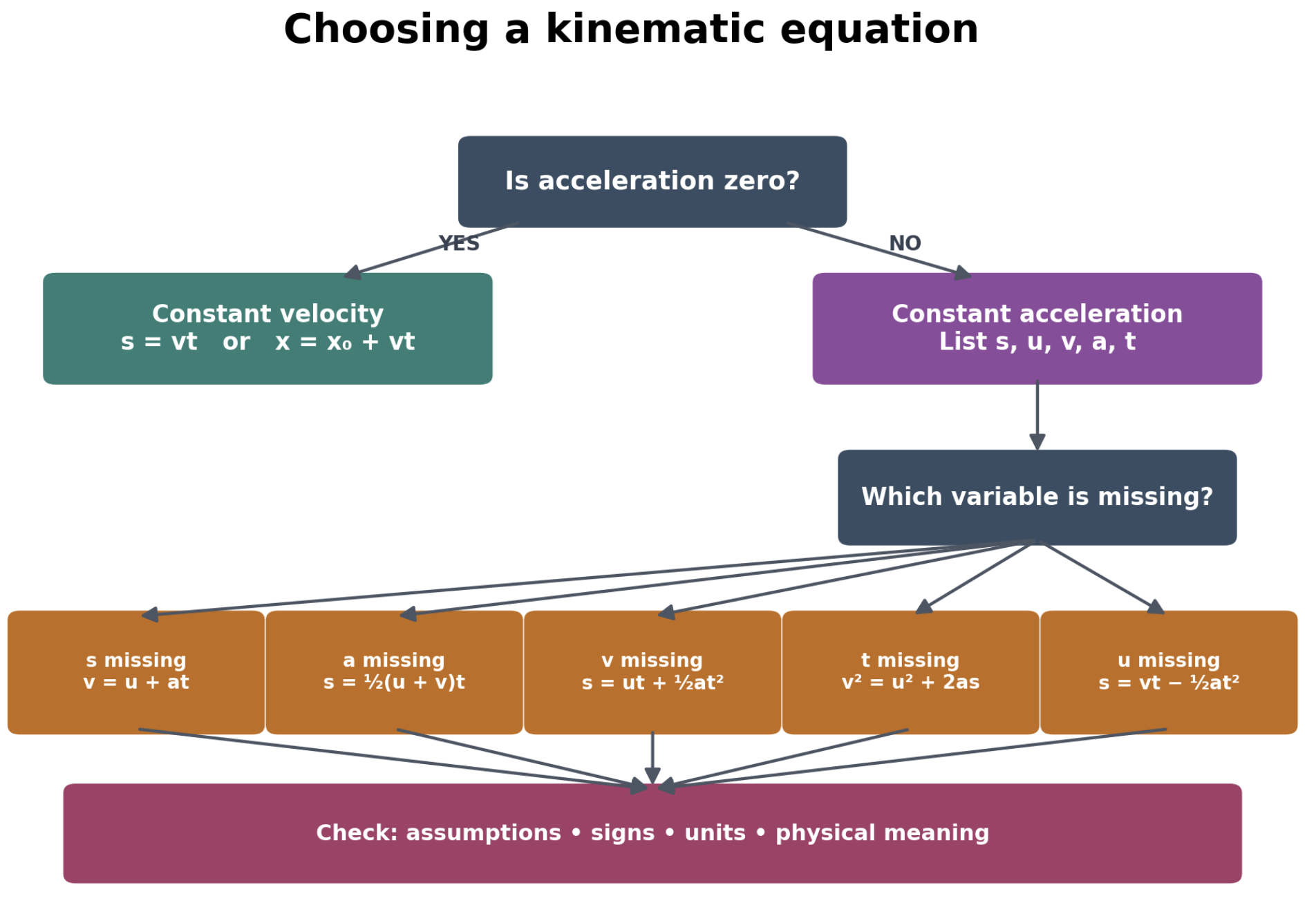
The missing-variable strategy
Each SUVAT equation leaves out one variable.
| Missing variable |
Most direct equation |
| s |
v = u + at |
| a |
s = ½(u + v)t |
| v |
s = ut + ½at² |
| t |
v² = u² + 2as |
| u |
s = vt − ½at² |
This table is a selection guide, rather than a rule that prevents other methods. Some problems can be solved using more than one equation.
The most efficient equation usually contains:
- All known variables needed for the solution.
- The required unknown.
- No additional unknowns.
When displacement is missing
If displacement is not given or required, use:
v = u + at
This equation connects initial velocity, final velocity, acceleration and time.
Worked example
A train increases its velocity uniformly from 12 m/s at 1.5 m/s² for 8 seconds. Calculate its final velocity.
Known:
u = 12 m/s
a = 1.5 m/s²
t = 8 s
v = ?
Displacement is not involved, so use:
v = u + at
v = 12 + 1.5(8)
v = 12 + 12
v = 24 m/s
Why this equation is suitable: It includes u, a, t and v, while leaving out the unneeded displacement s.
If acceleration is not given or required, use:
s = ½(u + v)t
This equation uses the average velocity for constant-acceleration motion.
Worked example
A cyclist accelerates uniformly from 4 m/s to 10 m/s over 6 seconds. Calculate the displacement.
Known:
u = 4 m/s
v = 10 m/s
t = 6 s
s = ?
Acceleration is not known or required, so use:
s = ½(u + v)t
s = ½(4 + 10)(6)
s = 7(6)
s = 42 m
Why this equation is suitable: It uses both velocities and time directly and does not require acceleration.
When final velocity is missing
If final velocity is not given or required, use:
s = ut + ½at²
Worked example
A skateboarder moves initially at 3 m/s and accelerates uniformly at 2 m/s² for 5 seconds. Calculate the displacement.
Known:
u = 3 m/s
a = 2 m/s²
t = 5 s
s = ?
Final velocity is not known, so use:
s = ut + ½at²
s = 3(5) + ½(2)(5²)
s = 15 + 25
s = 40 m
Why this equation is suitable: It contains the three known quantities and displacement, while leaving out v.
When time is missing
If time is not provided or required, use:
v² = u² + 2as
Worked example
A motorcycle accelerates uniformly from 8 m/s at 3 m/s² over 24 m. Calculate its final velocity.
Known:
u = 8 m/s
a = 3 m/s²
s = 24 m
v = ?
Time is absent, so use:
v² = u² + 2as
v² = 8² + 2(3)(24)
v² = 64 + 144
v² = 208
v = √208
v ≈ 14.4 m/s
The positive solution is appropriate because the motorcycle continues moving in the chosen positive direction.
Why this equation is suitable: It connects u, v, a and s without requiring time.
When initial velocity is missing
If initial velocity is not given or required, use:
s = vt − ½at²
Worked example
A vehicle reaches a final velocity of 20 m/s after accelerating uniformly at 2 m/s² for 6 seconds. Calculate its displacement during the interval.
Known:
v = 20 m/s
a = 2 m/s²
t = 6 s
s = ?
Initial velocity is absent, so use:
s = vt − ½at²
s = 20(6) − ½(2)(6²)
s = 120 − 36
s = 84 m
Why this equation is suitable: It contains v, a, t and s and leaves out the unknown initial velocity.
Choosing a constant-velocity equation
If acceleration is zero, the motion does not require the full SUVAT equations.
Worked example
A train travels east at a constant velocity of 18 m/s for 25 seconds. Calculate its displacement.
Known:
v = 18 m/s
t = 25 s
s = ?
Use:
s = vt
s = 18(25)
s = 450 m east
Why this equation is suitable: Velocity is constant, so displacement equals velocity multiplied by time.
Using an acceleration equation would add unnecessary variables.
Steady motion along a straight path can often be modelled using constant velocity. Brief starting, stopping and turning intervals require different models.
Choosing between similar equations
Sometimes more than one equation can solve a problem.
Suppose a car accelerates uniformly from 5 m/s to 17 m/s over 6 seconds, and displacement is required.
One direct approach is:
s = ½(u + v)t
s = ½(5 + 17)(6)
s = 66 m
A longer approach would be:
- Calculate acceleration using v = u + at.
- Substitute that acceleration into s = ut + ½at².
Both methods are valid, but the average-velocity equation is more efficient because it uses the provided information directly.
Efficiency means choosing a method that:
- Uses the fewest necessary steps.
- Avoids calculating quantities that were not requested.
- Reduces opportunities for arithmetic errors.
- Keeps the reasoning easy to follow.
Equation selection from graphical information
Graphs may provide variables without stating them directly.
Position–time graph
The gradient gives velocity:
v = Δx/Δt
A straight line represents constant velocity.
Velocity–time graph
The vertical coordinate gives velocity.
The gradient gives acceleration:
a = Δv/Δt
The area under the graph gives displacement.
The vertical coordinate gives acceleration.
The signed area gives change in velocity:
Δv = area under the graph
Graphical information can be combined with equations. For example, you may calculate acceleration from a velocity–time gradient and then use a SUVAT equation to find displacement.
Worked example using a graph description
A straight velocity–time line rises from 4 m/s at t = 0 to 16 m/s at t = 6 s. Find the acceleration and displacement.
a = (16 − 4)/(6 − 0)
a = 12/6
a = 2 m/s²
Displacement from the area
The area is a trapezium:
s = ½(u + v)t
s = ½(4 + 16)(6)
s = 10(6)
s = 60 m
The same equation appears both as a SUVAT equation and as the area of a trapezium under a velocity–time graph.
Recognizing free-fall situations
Near Earth’s surface, free fall is modelled using constant downward acceleration:
g ≈ 9.8 m/s²
If upward is positive:
a = −9.8 m/s²
If downward is positive:
a = +9.8 m/s²
The increasing separation between successive positions of a falling object shows that its velocity is changing.
Worked example: time is missing
A ball is thrown vertically upwards at 14 m/s. Calculate its maximum height above the release point. Ignore air resistance.
Choose upwards as positive.
At maximum height:
v = 0 m/s
Known:
u = +14 m/s
v = 0 m/s
a = −9.8 m/s²
s = ?
t is missing
Use:
v² = u² + 2as
0² = 14² + 2(−9.8)s
0 = 196 − 19.6s
19.6s = 196
s = 10 m
Why this equation is suitable: Time is not given or required, so the equation that omits t is the most direct choice.
Recognizing multi-stage motion
A single equation may not describe an entire journey.
For example, a car may:
- Accelerate uniformly for 5 seconds.
- Move at constant velocity for 10 seconds.
- Decelerate uniformly until it stops.
Each stage requires its own model.
| Stage |
Motion model |
Likely equations |
| Accelerating |
Constant acceleration |
SUVAT |
| Cruising |
Constant velocity |
s = vt |
| Braking |
Constant acceleration |
SUVAT |
The final velocity of one stage becomes the initial velocity of the next.
Calculate the displacement of each stage separately, then add the results.
Worked example: selecting equations for multiple stages
A car starts from rest and accelerates uniformly at 2 m/s² for 5 seconds. It then travels at constant velocity for 8 seconds.
Accelerating stage
Known:
u = 0 m/s
a = 2 m/s²
t = 5 s
First find the final velocity:
v = u + at
v = 0 + 2(5)
v = 10 m/s
Find the displacement:
s₁ = ut + ½at²
s₁ = 0 + ½(2)(5²)
s₁ = 25 m
Constant-velocity stage
The car now travels at 10 m/s for 8 seconds:
s₂ = vt
s₂ = 10(8)
s₂ = 80 m
Total displacement
s_total = 25 + 80
s_total = 105 m
One equation was not applied to the whole journey because the motion model changed after five seconds.
Situations where no standard equation applies directly
The SUVAT equations assume constant acceleration. They are not directly appropriate when:
- Acceleration changes continuously.
- A velocity–time graph is curved.
- Air resistance changes significantly.
- An engine provides varying acceleration.
- The motion follows several stages that have not been separated.
Possible approaches include:
- Dividing the motion into shorter stages.
- Using the gradient or area of a graph.
- Using calculus for continuously varying motion.
- Using numerical methods or computer models.
Identifying that an equation is unsuitable is part of good problem solving.
Explaining why an equation is suitable
A strong explanation identifies the variables and the motion condition.
For example:
“Acceleration is constant. The values of u, a and t are known, displacement s is required, and final velocity v is not given. Therefore, s = ut + ½at² is suitable because it contains the known variables and the required unknown but does not contain v.”
A weaker explanation would be:
“I used this equation because it has the right letters.”
A complete explanation should state:
- Why the motion model applies.
- Which variables are known.
- Which variable is required.
- Which variable is missing.
- Why the selected equation avoids unnecessary unknowns.
Checking signs before selecting an equation
Choosing the correct formula is not enough. Vector values also require correct signs.
Suppose a car moves right at 20 m/s and slows uniformly to 8 m/s in 4 seconds.
Choose right as positive:
u = +20 m/s
v = +8 m/s
t = 4 s
Its acceleration is:
a = (v − u)/t
a = (8 − 20)/4
a = −3 m/s²
Both velocities are positive because the car continues moving right. The acceleration is negative because it acts to the left.
Checking units
Convert measurements into compatible units before selecting and using an equation.
Common SI units are:
- Displacement: metres, m.
- Velocity: metres per second, m/s.
- Acceleration: metres per second squared, m/s².
- Time: seconds, s.
To convert:
km/h to m/s: divide by 3.6
m/s to km/h: multiply by 3.6
Worked example
A vehicle moving at 72 km/h accelerates uniformly at 2 m/s² for 5 seconds. Find its final velocity.
Convert the initial velocity:
u = 72/3.6
u = 20 m/s
Use:
v = u + at
v = 20 + 2(5)
v = 30 m/s
Checking an equation using dimensions
The terms in an equation must have compatible units.
For:
v = u + at
- u has units m/s.
- at has units (m/s²)(s) = m/s.
- v has units m/s.
The units are consistent.
For:
s = ut + ½at²
- ut has units (m/s)(s) = m.
- at² has units (m/s²)(s²) = m.
- s has units m.
Dimensional checking cannot prove that an equation is correct, but it can reveal many incorrect equations.
Common misconceptions
- “I should choose an equation before listing the variables.” List the variables first so the choice is based on evidence.
- “SUVAT can be used whenever velocity changes.” Acceleration must remain constant during the interval.
- “Constant speed always means constant velocity.” Direction must also remain unchanged.
- “The missing-variable table gives the only possible method.” It identifies the most direct standard equation.
- “Starting from rest means acceleration is zero.” It means initial velocity is zero.
- “Stopping means acceleration is zero.” It means final velocity is zero.
- “Negative acceleration always means slowing down.” Compare its direction with the velocity.
- “One equation must describe an entire journey.” Multi-stage motion may require several equations.
- “A correct formula guarantees a correct solution.” Signs, units, assumptions and interpretation must also be correct.
Did you know?
The five SUVAT equations are not five unrelated formulas. They are different combinations of the same relationships between velocity, acceleration, time and displacement.
For constant acceleration:
- The gradient of the velocity–time graph gives a.
- The area under the graph gives s.
- The graph begins at u and ends at v.
Understanding these connections makes equation selection easier than memorizing each equation in isolation.
Key terms
- Equation selection: Choosing a mathematical relationship suited to the available information and motion conditions.
- Constant velocity: Motion with unchanged speed and direction.
- Uniform acceleration: Motion with constant acceleration.
- SUVAT: The five variables displacement, initial velocity, final velocity, acceleration and time.
- Known variable: A quantity provided or determined from the problem.
- Unknown variable: A quantity that must be calculated.
- Missing variable: A SUVAT quantity absent from both the given information and the required result.
- Motion model: A mathematical description based on assumptions about the motion.
- Free fall: Motion in which gravity is the only significant force.
- Multi-stage motion: Motion divided into intervals with different conditions.
- Dimensional consistency: Agreement between the units of all terms in an equation.
Key takeaways
- Identify the motion model before selecting an equation.
- Use s = vt when velocity is constant.
- Use the SUVAT equations only when acceleration is constant.
- List s, u, v, a and t before calculating.
- Select an equation containing the known quantities and required unknown.
- Use the missing variable to identify the most direct SUVAT equation.
- Separate journeys into stages when the motion conditions change.
- Explain an equation choice using the variables and assumptions.
- Check signs, units and physical meaning after solving.