Advanced Applications and Mathematical Connections
1. Vectors in Calculus
Learning outcomes
- I can recognise vectors in differentiation and integration.
- I can describe vector-valued functions.
- I can interpret motion using vectors.
- I can analyse rates of change with vectors.
- I can connect vectors to multivariable mathematics.
Introduction
Calculus is the mathematics of change. It allows us to investigate how quantities vary, calculate instantaneous rates of change, and determine accumulated quantities.
Vectors extend these ideas into two and three dimensions.
When an object moves along a curved path, its position, velocity, and acceleration may all change. A single number cannot fully describe this motion because direction is just as important as magnitude.
For example, a spacecraft travelling around a planet may maintain a constant speed while continuously changing direction. A ball thrown through the air changes both its horizontal and vertical position. A robot arm moves through three-dimensional space, requiring several coordinates to describe its position.
Vector calculus provides the mathematical tools needed to analyse these situations.
It is used in:
-
Physics and mechanics
-
Projectile motion
-
Circular and orbital motion
-
Engineering and robotics
-
Fluid dynamics
-
Electromagnetism
-
Computer graphics
-
Weather forecasting
-
Optimisation and multivariable mathematics
In this lesson, we will investigate vector-valued functions, vector differentiation, vector integration, motion in two and three dimensions, and connections to multivariable calculus.
What Is a Vector-Valued Function?
A vector-valued function is a function whose output is a vector rather than a single number.
An ordinary function might be:
f(t) = t²
For every value of t, the function produces one number.
A vector-valued function produces two or more components.
For example:
This function gives a position in two-dimensional space for each value of t.
We can also write:
where:
-
i is the unit vector in the positive x-direction.
-
j is the unit vector in the positive y-direction.
-
t is the independent variable, often representing time.
For three-dimensional motion:
Here, k is the unit vector in the positive z-direction.
Worked Example 1: Evaluating a Vector-Valued Function
An object has position:
Find its position at t = 2.
Substitute t = 2 into each component.
x(2) = 2(2) + 1 = 5
y(2) = 2² − 3 = 1
Therefore:
The object's position is (5, 1).
At t = 0:
x(0) = 1
y(0) = −3
Therefore, the object moves from (1, −3) at t = 0 to (5, 1) at t = 2.
Vector-Valued Functions Describe Curves
A vector-valued function can describe the path followed by a moving object.
Consider:
The component equations are:
x = t
y = t²
Since t = x:
The path is a parabola.
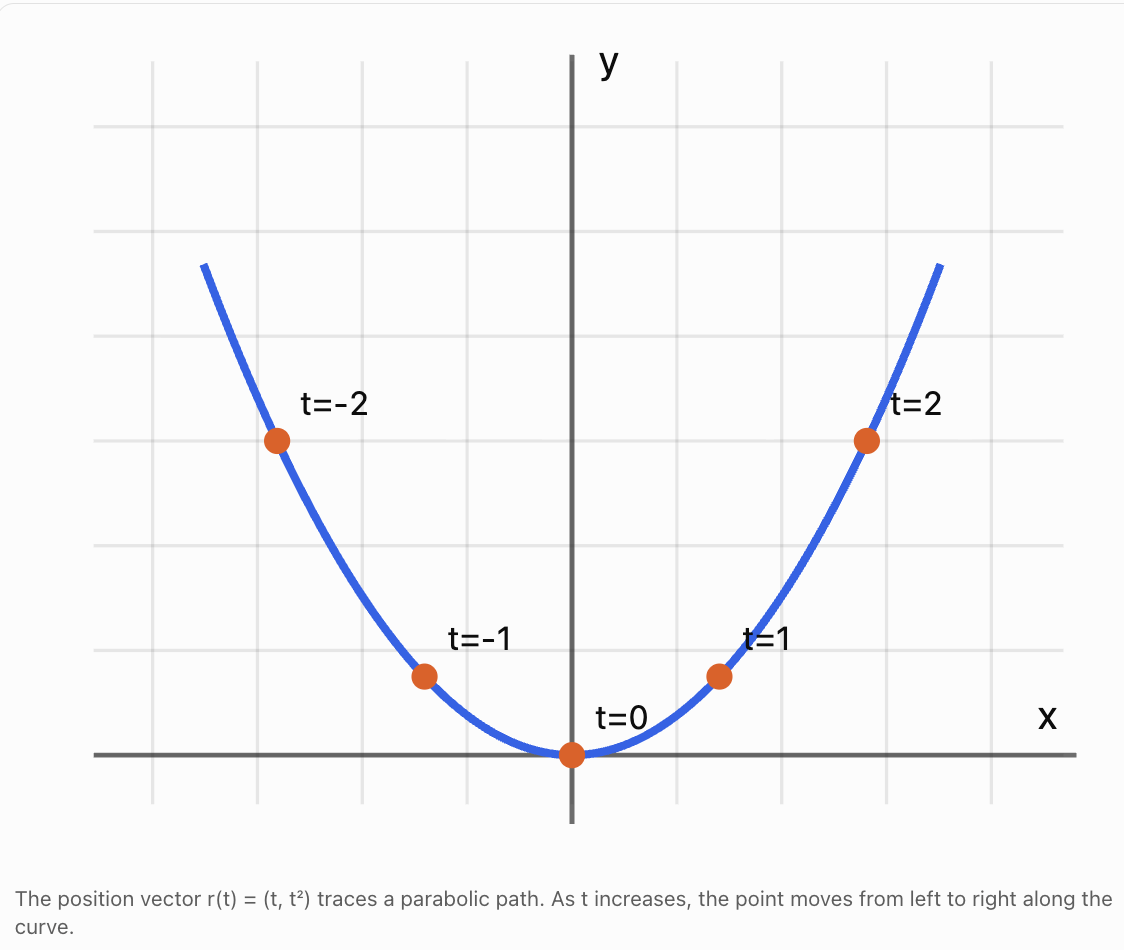
A vector-valued function describes both the shape of the path and the position of the object at each time.
This is an important distinction.
The equation y = x² describes the curve itself, while r(t) = (t, t²) also describes how the object moves along it as t changes.
Differentiating Vector-Valued Functions
Differentiation measures instantaneous rates of change.
For a scalar function:
For a vector-valued function, we differentiate each component separately.
If:
then:
The derivative is itself a vector.
Worked Example 2: Differentiating a Vector Function
Given:
Differentiate each component.
For the x-component:
For the y-component:
Therefore:
At t = 1:
This derivative describes the instantaneous rate of change of the position vector at t = 1.
Position, Velocity, and Acceleration
One of the most important applications of vector calculus is the study of motion.
Position Vector
The position vector describes where an object is located relative to an origin.
Velocity Vector
Velocity is the rate of change of position.
Therefore:
Velocity includes both magnitude and direction.
Acceleration Vector
Acceleration is the rate of change of velocity.
Therefore:
These relationships are fundamental in mechanics.
Position
\(\mathbf r(t)\)metres (m)
Velocity
\(\mathbf v(t)\)m/s
Acceleration
\(\mathbf a(t)\)m/s²
Differentiate to move from position to velocity to acceleration.
Worked Example 3: Position, Velocity, and Acceleration
A particle moves according to:
Find:
a) The velocity vector.
b) The acceleration vector.
c) The velocity and acceleration at t = 2 s.
Part a: Velocity
Differentiate position:
Part b: Acceleration
Differentiate velocity:
Part c: At t = 2
Velocity:
Acceleration:
The particle has a velocity directed right and upward, and its acceleration also has positive horizontal and vertical components.
Speed and the Magnitude of Velocity
Velocity is a vector, while speed is a scalar.
Speed is the magnitude of the velocity vector.
For two-dimensional motion:
For three-dimensional motion:
Worked Example 4: Calculating Speed
A particle has velocity:
Calculate its speed.
The speed is 10 m/s.
The direction of motion can also be calculated:
Therefore, the particle moves at 10 m/s, approximately 53.1° above the positive x-axis.
Velocity Is Tangent to the Path
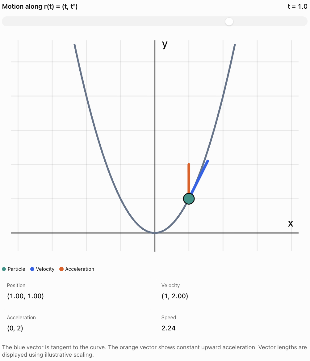
The velocity vector points in the instantaneous direction of motion.
Geometrically, it is tangent to the curve traced by the position vector, provided the velocity is nonzero.
Consider:
Differentiate:
At t = 1:
The particle is at (1, 1), and its velocity points in the direction (1, 2).
This agrees with the gradient of the curve y = x² at x = 1:
The velocity vector has gradient:
The results agree.
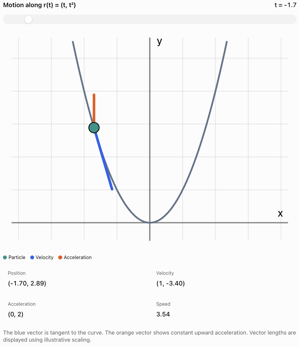
Interactive Vector Motion Explorer
Adjust time to see how a particle's position, velocity, and acceleration change along a parabolic path.
Integrating Vector-Valued Functions
Integration reverses differentiation.
If velocity is known, integration can be used to find position.
If acceleration is known, integration can be used to find velocity.
A vector-valued function is integrated component by component.
If:
then:
Here, C is a constant vector.
For motion:
with the constant vector determined by the initial position.
Similarly:
with the constant vector determined by the initial velocity.
Worked Example 5: Finding Position from Velocity
A particle has velocity:
Its initial position is:
Find its position function.
Step 1: Integrate the x-component.
Step 2: Integrate the y-component.
Therefore:
Step 3: Use the initial position.
At t = 0:
Since:
we obtain:
C₁ = 3
C₂ = −1
Therefore:
Definite Integrals and Displacement
The definite integral of velocity gives displacement.
Displacement is the change in position:
Worked Example 6: Calculating Displacement
A particle has velocity:
Calculate its displacement from t = 1 s to t = 3 s.
Integrate:
Evaluate:
x-displacement:
3² − 1² = 8
y-displacement:
3³ − 1³ = 26
Therefore:
The magnitude of the displacement is:
This is the straight-line distance between the initial and final positions, not necessarily the total distance travelled along the path.
Distance Travelled and Arc Length
Displacement and distance travelled are different quantities.
Displacement depends only on the initial and final positions.
Distance travelled measures the total length of the path.
For a vector-valued position function:
the total distance travelled from t = a to t = b is:
In three dimensions:
This is also called the arc length of the path.
Worked Example 7: Distance Along a Straight Path
A particle has velocity:
for 0 ≤ t ≤ 5.
Calculate the total distance travelled.
First find the speed:
Then:
Because the velocity is constant, the particle travels in a straight line without changing direction.
Its displacement magnitude is also 25 m.
For curved motion, the total distance travelled is generally greater than the displacement magnitude.
Projectile Motion Using Vectors
Projectile motion is an important application of vector calculus.
When air resistance is neglected, a projectile experiences constant downward acceleration due to gravity.
Taking upward as positive:
where g ≈ 9.81 m/s² near Earth's surface.
Integrating acceleration gives velocity:
Integrating velocity gives position:
For a projectile launched with speed u at angle θ above the horizontal:
v₀ₓ = u cos θ
v₀ᵧ = u sin θ
Therefore:
Worked Example 8: Projectile Motion
A ball is launched from ground level with initial speed 20 m/s at 30° above the horizontal.
Ignore air resistance.
Find:
a) The position vector after 2 s.
b) The velocity vector after 2 s.
c) The speed after 2 s.
Use g = 9.81 m/s².
Part a: Position
Horizontal initial velocity:
Vertical initial velocity:
Horizontal position after 2 s:
x = 17.32(2)
x ≈ 34.64 m
Vertical position:
y = 20 − 19.62
y = 0.38 m
Therefore:
Part b: Velocity
Horizontal velocity remains constant:
vₓ = 17.32 m/s
Vertical velocity:
vᵧ = −9.62 m/s
Therefore:
The ball is moving rightward and downward.
Part c: Speed
The speed is approximately 19.8 m/s.
Circular Motion Using Vector Functions
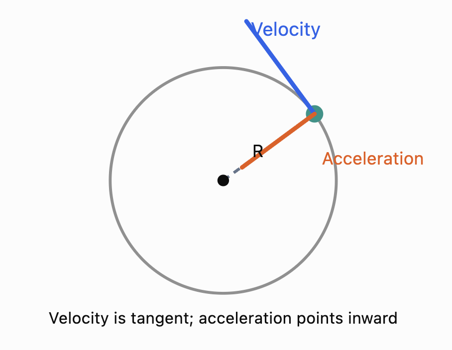
Vectors are especially important in circular motion because the direction of velocity continuously changes.
Consider an object moving around a circle of radius R with constant angular speed ω.
Its position vector is:
Differentiate to find velocity:
Differentiate again:
Notice:
The acceleration points in the opposite direction to the position vector.
Therefore, it points toward the centre of the circle.
This is centripetal acceleration.
Its magnitude is:
Worked Example 9: Circular Motion
An object moves in a circle of radius 5 m with angular speed 2 rad/s.
Calculate:
a) Its speed.
b) Its centripetal acceleration.
Part a: Speed
Part b: Centripetal acceleration
Even though the speed is constant, the object accelerates because its direction changes continuously.
The Unit Tangent Vector
The velocity vector points in the direction of motion.
To describe direction without including speed, we use the unit tangent vector.
This vector has magnitude 1.
Worked Example 10: Unit Tangent Vector
Suppose:
Then:
Its magnitude is:
Therefore:
The unit tangent vector describes the direction of motion independently of speed.
Tangential and Normal Acceleration
Acceleration can change an object's speed, direction, or both.
It is useful to divide acceleration into two components:
-
Tangential acceleration: changes speed.
-
Normal acceleration: changes direction.
For a particle moving along a smooth curve:
where:
-
T is the unit tangent vector.
-
N is the principal unit normal vector, when defined.
-
a_T is tangential acceleration.
-
a_N is normal acceleration.
The tangential component is:
The normal component is related to curvature:
where R_c is the local radius of curvature.
For circular motion, R_c is the radius of the circle.
This decomposition is useful in vehicle dynamics, roller-coaster design, aerospace engineering, and robotics.
Connecting Vectors to Multivariable Calculus
So far, we have studied vector-valued functions that depend on one variable, usually time.
Multivariable calculus studies functions that depend on two or more independent variables.
For example:
This function assigns a scalar value to each point (x, y).
It can represent a surface in three-dimensional space:
Partial Derivatives
A partial derivative measures how a multivariable function changes with respect to one variable while holding the others constant.
For:
The partial derivative with respect to x is:
The partial derivative with respect to y is:
These describe how the surface changes in the x- and y-directions.
The Gradient Vector
The gradient combines the partial derivatives of a scalar function into a vector.
For:
the gradient is:
For three variables:
The gradient points in the direction of greatest local increase of the function.
Its magnitude gives the maximum rate of increase per unit distance.
Worked Example 11: Calculating a Gradient
Given:
Find the gradient at (1, 2).
Step 1: Differentiate with respect to x.
Step 2: Differentiate with respect to y.
Therefore:
At (1, 2):
x-component:
6(1) + 2(2) = 10
y-component:
2(1) + 2(2) = 6
Therefore:
The function increases most rapidly in the direction (10, 6) at this point.
Directional Derivatives
The gradient tells us the direction of greatest increase, but what if we want the rate of change in another direction?
This is measured using a directional derivative.
For a unit vector u:
The dot product determines the rate of change in the chosen direction.
Worked Example 12: Directional Derivative
Suppose:
We want the rate of change in the direction:
Calculate:
The function increases at a rate of 10 units per unit distance in the specified direction.
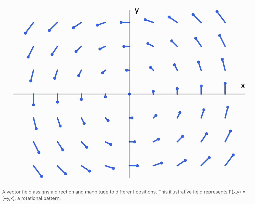
Vector Fields
A vector field assigns a vector to every point in a region.
For example, a wind field may describe the velocity of air at different locations.
Possible vector fields include:
-
Wind velocity.
-
Water flow.
-
Gravitational fields.
-
Electric fields.
-
Magnetic fields.
-
Force fields.
Worked Example 13: Evaluating a Vector Field
Suppose:
\[ \mathbf F(x,y)=2x\mathbf i-3y\mathbf j \]Find the vector at (2, −1).
Substitute:
\[ \mathbf F(2,-1)=2(2)\mathbf i-3(-1)\mathbf j \]Therefore:
\[ \boxed{\mathbf F(2,-1)=4\mathbf i+3\mathbf j} \]The vector points right and upward.
Its magnitude is:
\[ |\mathbf F|=\sqrt{4^2+3^2}=5 \]The Chain Rule for Motion Through a Scalar Field
Vector calculus also connects motion to changing physical conditions.
Suppose the temperature in a room depends on position:
T = T(x, y)
A moving sensor follows a path:
\[ \mathbf r(t)=x(t)\mathbf i+y(t)\mathbf j \]The temperature experienced by the sensor changes as it moves.
The multivariable chain rule gives:
\[ \boxed{ \frac{dT}{dt}= \frac{\partial T}{\partial x}\frac{dx}{dt}+ \frac{\partial T}{\partial y}\frac{dy}{dt} } \]In vector form:
\[ \boxed{\frac{dT}{dt}=\nabla T\cdot\mathbf v} \]This formula connects the temperature gradient with the sensor's velocity.
Worked Example 14: Moving Through a Temperature Field
Suppose:
\[ T(x,y)=20+2x+3y \]A sensor moves with velocity:
\[ \mathbf v=4\mathbf i+\mathbf j\text{ m/s} \]Find the rate of change of temperature experienced by the sensor.
First calculate the gradient:
\[ \nabla T=2\mathbf i+3\mathbf j \]Then:
\[ \frac{dT}{dt}=\nabla T\cdot\mathbf v \]\[ =2(4)+3(1) \]\[ \boxed{\frac{dT}{dt}=11^\circ\text{C/s}} \]The sensor experiences a temperature increase of 11°C per second under this idealised model.
This type of calculation is useful in environmental science, fluid dynamics, and heat transfer.
The Jacobian Matrix
For functions with several inputs and several outputs, derivatives can be organised into a matrix called the Jacobian.
Suppose:
\[ \mathbf F(x,y)= \begin{bmatrix} f(x,y)\\ g(x,y) \end{bmatrix} \]The Jacobian matrix is:
\[ \boxed{ J= \begin{bmatrix} \frac{\partial f}{\partial x}&\frac{\partial f}{\partial y}\\ \frac{\partial g}{\partial x}&\frac{\partial g}{\partial y} \end{bmatrix} } \]The Jacobian describes how small changes in the inputs affect the outputs.
Worked Example 15: Calculating a Jacobian
Given:
\[ \mathbf F(x,y)= \begin{bmatrix} x^2+y\\ xy \end{bmatrix} \]Calculate the Jacobian.
For the first component:
f(x, y) = x² + y
\[ \frac{\partial f}{\partial x}=2x \]\[ \frac{\partial f}{\partial y}=1 \]For the second component:
g(x, y) = xy
\[ \frac{\partial g}{\partial x}=y \]\[ \frac{\partial g}{\partial y}=x \]Therefore:
\[ \boxed{ J(x,y)= \begin{bmatrix} 2x&1\\ y&x \end{bmatrix} } \]At (2, 3):
\[ \boxed{ J(2,3)= \begin{bmatrix} 4&1\\ 3&2 \end{bmatrix} } \]The Jacobian is widely used in robotics, optimisation, coordinate transformations, and numerical methods.
Real-World Applications of Vector Calculus
Orbital Mechanics
Vector functions describe the positions and velocities of satellites and spacecraft. Differentiation determines velocity and acceleration, while integration predicts future motion from known forces.
Fluid Dynamics
Engineers model air and water movement using vector fields. Velocity, acceleration, pressure gradients, and fluid-flow rates are analysed using vector calculus.
Robotics
Vector-valued functions describe robot trajectories. Derivatives determine tool velocities and accelerations, while Jacobian matrices connect joint movement to end-effector motion.
Meteorology
Wind velocity is a vector field. Weather models use spatial derivatives and time-dependent equations to describe changes in atmospheric conditions.
Electromagnetism
Electric and magnetic fields are vector fields. Advanced vector calculus describes how these fields vary through space and time.
Common Mistakes
Mistake 1: Differentiating the magnitude instead of the vector components
Differentiate each component of the vector-valued function separately.
Mistake 2: Confusing speed and velocity
Speed is a scalar. Velocity is a vector containing magnitude and direction.
Mistake 3: Assuming constant speed means zero acceleration
An object moving in a circle at constant speed still accelerates because its direction changes.
Mistake 4: Forgetting the constant vector when integrating
Each component may have its own integration constant. Together, these form a constant vector.
Mistake 5: Confusing displacement with distance travelled
Displacement is the change in position. Distance travelled is the length of the path.
Mistake 6: Assuming velocity and acceleration always point in the same direction
Acceleration may point in a different direction from velocity.
Mistake 7: Forgetting units
Position is measured in metres, velocity in m/s, and acceleration in m/s².
Mistake 8: Confusing scalar functions and vector-valued functions
A scalar function produces a number. A vector-valued function produces a vector.
Mistake 9: Treating the gradient as a scalar
The gradient is a vector composed of partial derivatives.
Mistake 10: Forgetting to use a unit vector in directional derivatives
The formula Dᵤf = ∇f · u assumes u has magnitude 1.
Mistake 11: Confusing partial derivatives with ordinary derivatives
A partial derivative varies one independent variable while holding the others fixed.
Mistake 12: Assuming a mathematical model always describes physical reality perfectly
Vector models may neglect friction, air resistance, changing forces, and other real-world effects.
Key Terms
-
Vector-Valued Function: Function that produces a vector as its output.
-
Position Vector: Vector describing an object's position relative to an origin.
-
Velocity Vector: Rate of change of position with respect to time.
-
Acceleration Vector: Rate of change of velocity with respect to time.
-
Speed: Magnitude of the velocity vector.
-
Vector Derivative: Derivative obtained by differentiating vector components.
-
Vector Integral: Integral obtained by integrating vector components.
-
Displacement: Change in position between two points.
-
Distance Travelled: Total length of the path followed.
-
Arc Length: Length of a curve over a specified interval.
-
Parametric Curve: Curve described by coordinate functions of a parameter.
-
Tangent Vector: Vector pointing along a curve.
-
Unit Tangent Vector: Tangent vector with magnitude 1.
-
Normal Vector: Vector perpendicular to the tangent direction.
-
Tangential Acceleration: Component of acceleration that changes speed.
-
Normal Acceleration: Component of acceleration that changes direction.
-
Centripetal Acceleration: Acceleration directed toward the centre of circular motion.
-
Angular Speed: Rate of change of angular position.
-
Scalar Field: Function assigning a scalar to every point in a region.
-
Vector Field: Function assigning a vector to every point in a region.
-
Partial Derivative: Derivative with respect to one variable while others remain fixed.
-
Gradient: Vector containing the partial derivatives of a scalar field.
-
Directional Derivative: Rate of change of a scalar function in a specified direction.
-
Multivariable Chain Rule: Rule for differentiating a function that depends on several changing variables.
-
Jacobian Matrix: Matrix of first-order partial derivatives of a vector-valued function.
-
Curvature: Measure of how sharply a curve changes direction.
-
Line Integral: Integral evaluated along a curve.
-
Vector Calculus: Branch of mathematics combining vector methods with differentiation and integration.
Key Takeaways
-
Vector-valued functions describe positions and other vector quantities that change with a parameter.
-
A position vector can describe motion along a curve in two or three dimensions.
-
Differentiating position gives velocity.
-
Differentiating velocity gives acceleration.
-
Speed is the magnitude of velocity.
-
Velocity is tangent to the path of motion when it is nonzero.
-
Integrating acceleration gives velocity, subject to an initial velocity.
-
Integrating velocity gives position, subject to an initial position.
-
Definite integration of velocity gives displacement.
-
Integrating speed gives total distance travelled.
-
Circular motion can involve constant speed but nonzero acceleration.
-
The gradient describes the direction and rate of greatest local increase of a scalar field.
-
Directional derivatives measure change in specified directions.
-
Vector fields describe quantities such as wind velocity, fluid flow, and electromagnetic fields.
-
Jacobian matrices connect vector functions to multivariable differentiation.
-
Vector calculus is essential in physics, engineering, robotics, and scientific modelling.
Check Your Understanding
Questions
Question 1: Vector-Valued Functions
Given:
\[ \mathbf r(t)=(3t+2)\mathbf i+(t^2-1)\mathbf j \]Find the position at t = 2.
Question 2: Vector Differentiation
Differentiate:
\[ \mathbf r(t)=t^3\mathbf i+(4t^2-3t)\mathbf j \]Question 3: Velocity and Acceleration
A particle moves according to:
\[ \mathbf r(t)=2t^2\mathbf i+(t^3-2t)\mathbf j \]Find its velocity and acceleration functions.
Question 4: Instantaneous Velocity
For the particle in Question 3, calculate the velocity at t = 2 s.
Question 5: Speed
A particle has velocity:
\[ \mathbf v=5\mathbf i+12\mathbf j \]Calculate its speed.
Question 6: Vector Integration
Integrate:
\[ \mathbf v(t)=6t\mathbf i+4t^3\mathbf j \]Question 7: Initial Conditions
A particle has velocity:
\[ \mathbf v(t)=2t\mathbf i+3\mathbf j \]Its initial position is:
\[ \mathbf r(0)=4\mathbf i-2\mathbf j \]Find its position function.
Question 8: Displacement
A particle has velocity:
\[ \mathbf v(t)=4t\mathbf i+2\mathbf j \]Calculate its displacement from t = 0 to t = 3.
Question 9: Circular Motion
An object moves in a circle of radius 4 m with angular speed 3 rad/s.
Calculate its speed and centripetal acceleration.
Question 10: Unit Tangent Vector
Given:
\[ \mathbf v=8\mathbf i+6\mathbf j \]Find the unit tangent vector.
Question 11: Partial Derivatives
Given:
\[ f(x,y)=4x^2+3xy+y^2 \]Find both first-order partial derivatives.
Question 12: Gradient
For the function in Question 11, calculate the gradient at (1, 2).
Question 13: Directional Derivative
A scalar field has gradient:
\[ \nabla f=3\mathbf i+4\mathbf j \]Calculate the directional derivative in the direction:
\[ \mathbf u=\frac35\mathbf i+\frac45\mathbf j \]Question 14: Vector Field
Given:
\[ \mathbf F(x,y)=x^2\mathbf i+2y\mathbf j \]Calculate the field vector at (2, −3).
Question 15: Integrated Motion Problem
A particle moves according to:
\[ \mathbf r(t)=(t^3-3t)\mathbf i+(2t^2+1)\mathbf j \]a) Find the velocity vector.
b) Find the acceleration vector.
c) Calculate the position at t = 2.
d) Calculate the velocity at t = 2.
e) Calculate the speed at t = 2.
f) Calculate the displacement from t = 0 to t = 2.
g) Explain the difference between the displacement magnitude and total distance travelled.
Fully Worked Answers
Answer 1: Vector-Valued Functions
Given:
\[ \mathbf r(t)=(3t+2)\mathbf i+(t^2-1)\mathbf j \]At t = 2:
x = 3(2) + 2 = 8
y = 2² − 1 = 3
Therefore:
\[ \boxed{\mathbf r(2)=8\mathbf i+3\mathbf j} \]Answer 2: Vector Differentiation
Differentiate each component:
\[ \frac{d}{dt}(t^3)=3t^2 \]\[ \frac{d}{dt}(4t^2-3t)=8t-3 \]Therefore:
\[ \boxed{\mathbf r'(t)=3t^2\mathbf i+(8t-3)\mathbf j} \]Answer 3: Velocity and Acceleration
Given:
\[ \mathbf r(t)=2t^2\mathbf i+(t^3-2t)\mathbf j \]Differentiate:
\[ \boxed{\mathbf v(t)=4t\mathbf i+(3t^2-2)\mathbf j} \]Differentiate again:
\[ \boxed{\mathbf a(t)=4\mathbf i+6t\mathbf j} \]Answer 4: Instantaneous Velocity
From Question 3:
\[ \mathbf v(t)=4t\mathbf i+(3t^2-2)\mathbf j \]At t = 2:
x-component:
4(2) = 8
y-component:
3(2²) − 2 = 10
Therefore:
\[ \boxed{\mathbf v(2)=8\mathbf i+10\mathbf j\text{ m/s}} \]Answer 5: Speed
\[ \mathbf v=5\mathbf i+12\mathbf j \]\[ |\mathbf v|=\sqrt{5^2+12^2} \]\[ =\sqrt{25+144} \]\[ =\sqrt{169} \]\[ \boxed{|\mathbf v|=13} \]If velocity is measured in m/s, the speed is 13 m/s.
Answer 6: Vector Integration
\[ \mathbf v(t)=6t\mathbf i+4t^3\mathbf j \]Integrate each component:
\[ \int6t\,dt=3t^2+C_1 \]\[ \int4t^3\,dt=t^4+C_2 \]Therefore:
\[ \boxed{\mathbf r(t)=3t^2\mathbf i+t^4\mathbf j+\mathbf C} \]where C is a constant vector.
Answer 7: Initial Conditions
Given:
\[ \mathbf v(t)=2t\mathbf i+3\mathbf j \]Integrate:
\[ \mathbf r(t)=(t^2+C_1)\mathbf i+(3t+C_2)\mathbf j \]Initial position:
\[ \mathbf r(0)=4\mathbf i-2\mathbf j \]Therefore:
C₁ = 4
C₂ = −2
Hence:
\[ \boxed{\mathbf r(t)=(t^2+4)\mathbf i+(3t-2)\mathbf j} \]Answer 8: Displacement
\[ \Delta\mathbf r=\int_0^3(4t\mathbf i+2\mathbf j)\,dt \]Integrate:
\[ \Delta\mathbf r=[2t^2]_0^3\mathbf i+[2t]_0^3\mathbf j \]x-displacement:
2(3²) = 18
y-displacement:
2(3) = 6
Therefore:
\[ \boxed{\Delta\mathbf r=18\mathbf i+6\mathbf j} \]Answer 9: Circular Motion
Given:
R = 4 m
ω = 3 rad/s
Speed:
\[ v=R\omega \]\[ v=4(3) \]\[ \boxed{v=12\text{ m/s}} \]Centripetal acceleration:
\[ a_c=R\omega^2 \]\[ a_c=4(3)^2 \]\[ \boxed{a_c=36\text{ m/s}^2} \]Answer 10: Unit Tangent Vector
Given:
\[ \mathbf v=8\mathbf i+6\mathbf j \]Magnitude:
\[ |\mathbf v|=\sqrt{8^2+6^2}=10 \]Therefore:
\[ \mathbf T=\frac{\mathbf v}{|\mathbf v|} \]\[ \boxed{\mathbf T=\frac45\mathbf i+\frac35\mathbf j} \]Answer 11: Partial Derivatives
Given:
\[ f(x,y)=4x^2+3xy+y^2 \]Differentiate with respect to x:
\[ \boxed{\frac{\partial f}{\partial x}=8x+3y} \]Differentiate with respect to y:
\[ \boxed{\frac{\partial f}{\partial y}=3x+2y} \]Answer 12: Gradient
The gradient is:
\[ \nabla f=(8x+3y)\mathbf i+(3x+2y)\mathbf j \]At (1, 2):
x-component:
8(1) + 3(2) = 14
y-component:
3(1) + 2(2) = 7
Therefore:
\[ \boxed{\nabla f(1,2)=14\mathbf i+7\mathbf j} \]Answer 13: Directional Derivative
Given:
\[ \nabla f=3\mathbf i+4\mathbf j \]and:
\[ \mathbf u=\frac35\mathbf i+\frac45\mathbf j \]Calculate:
\[ D_{\mathbf u}f=\nabla f\cdot\mathbf u \]\[ =3\left(\frac35\right)+4\left(\frac45\right) \]\[ =\frac95+\frac{16}{5} \]\[ =\frac{25}{5} \]\[ \boxed{D_{\mathbf u}f=5} \]Answer 14: Vector Field
Given:
\[ \mathbf F(x,y)=x^2\mathbf i+2y\mathbf j \]At (2, −3):
x-component:
2² = 4
y-component:
2(−3) = −6
Therefore:
\[ \boxed{\mathbf F(2,-3)=4\mathbf i-6\mathbf j} \]Answer 15: Integrated Motion Problem
Given:
\[ \mathbf r(t)=(t^3-3t)\mathbf i+(2t^2+1)\mathbf j \]Part a: Velocity
Differentiate:
\[ \boxed{\mathbf v(t)=(3t^2-3)\mathbf i+4t\mathbf j} \]Part b: Acceleration
Differentiate velocity:
\[ \boxed{\mathbf a(t)=6t\mathbf i+4\mathbf j} \]Part c: Position at t = 2
x-component:
2³ − 3(2) = 8 − 6 = 2
y-component:
2(2²) + 1 = 9
Therefore:
\[ \boxed{\mathbf r(2)=2\mathbf i+9\mathbf j} \]Part d: Velocity at t = 2
x-component:
3(2²) − 3 = 9
y-component:
4(2) = 8
Therefore:
\[ \boxed{\mathbf v(2)=9\mathbf i+8\mathbf j} \]Part e: Speed at t = 2
\[ |\mathbf v(2)|=\sqrt{9^2+8^2} \]\[ =\sqrt{145} \]\[ \boxed{|\mathbf v(2)|\approx12.04} \]Part f: Displacement from t = 0 to t = 2
Initial position:
\[ \mathbf r(0)=0\mathbf i+1\mathbf j \]Final position:
\[ \mathbf r(2)=2\mathbf i+9\mathbf j \]Therefore:
\[ \Delta\mathbf r=\mathbf r(2)-\mathbf r(0) \]\[ \boxed{\Delta\mathbf r=2\mathbf i+8\mathbf j} \]Magnitude:
\[ |\Delta\mathbf r|=\sqrt{2^2+8^2} \]\[ =\sqrt{68} \]\[ \boxed{|\Delta\mathbf r|\approx8.25} \]Part g: Displacement versus distance
The displacement magnitude is approximately 8.25 units.
However, the particle follows a curved path, so the total distance travelled is greater than the straight-line displacement.
The distance travelled would be calculated using:
\[ s=\int_0^2|\mathbf v(t)|\,dt \]Therefore:
\[ \boxed{ s=\int_0^2\sqrt{(3t^2-3)^2+(4t)^2}\,dt } \]This integral gives the total arc length of the path and can be evaluated numerically.
Final Reflection
Vector calculus extends ordinary differentiation and integration into two and three dimensions.
Vector-valued functions allow us to describe motion along curved paths. Differentiation gives velocity and acceleration, while integration allows us to calculate displacement and recover position from known motion.
The geometric interpretation is equally important. Velocity is tangent to the path, while acceleration may change speed, direction, or both. Circular motion provides a clear example of acceleration occurring even when speed remains constant.
Vector calculus also provides the foundation for multivariable mathematics. Gradients, directional derivatives, vector fields, and Jacobian matrices allow scientists to investigate how quantities change across space.
These ideas are essential in physics, engineering, robotics, fluid dynamics, meteorology, electromagnetism, and many other fields.
The central idea is that vector calculus combines magnitude, direction, and rates of change to describe and analyse motion and physical systems in multiple dimensions.
-