Advanced Applications and Mathematical Connections
| サイト: | Young Education |
| コース: | Vectors and Matrices |
| ブック: | Advanced Applications and Mathematical Connections |
| 印刷者: | Guest user |
| 日付: | 2026年 11月 9日(月曜日) 16:36 |
1. Vectors in Calculus
Learning outcomes
- I can recognise vectors in differentiation and integration.
- I can describe vector-valued functions.
- I can interpret motion using vectors.
- I can analyse rates of change with vectors.
- I can connect vectors to multivariable mathematics.
Introduction
Calculus is the mathematics of change. It allows us to investigate how quantities vary, calculate instantaneous rates of change, and determine accumulated quantities.
Vectors extend these ideas into two and three dimensions.
When an object moves along a curved path, its position, velocity, and acceleration may all change. A single number cannot fully describe this motion because direction is just as important as magnitude.
For example, a spacecraft travelling around a planet may maintain a constant speed while continuously changing direction. A ball thrown through the air changes both its horizontal and vertical position. A robot arm moves through three-dimensional space, requiring several coordinates to describe its position.
Vector calculus provides the mathematical tools needed to analyse these situations.
It is used in:
-
Physics and mechanics
-
Projectile motion
-
Circular and orbital motion
-
Engineering and robotics
-
Fluid dynamics
-
Electromagnetism
-
Computer graphics
-
Weather forecasting
-
Optimisation and multivariable mathematics
In this lesson, we will investigate vector-valued functions, vector differentiation, vector integration, motion in two and three dimensions, and connections to multivariable calculus.
What Is a Vector-Valued Function?
A vector-valued function is a function whose output is a vector rather than a single number.
An ordinary function might be:
f(t) = t²
For every value of t, the function produces one number.
A vector-valued function produces two or more components.
For example:
This function gives a position in two-dimensional space for each value of t.
We can also write:
where:
-
i is the unit vector in the positive x-direction.
-
j is the unit vector in the positive y-direction.
-
t is the independent variable, often representing time.
For three-dimensional motion:
Here, k is the unit vector in the positive z-direction.
Worked Example 1: Evaluating a Vector-Valued Function
An object has position:
Find its position at t = 2.
Substitute t = 2 into each component.
x(2) = 2(2) + 1 = 5
y(2) = 2² − 3 = 1
Therefore:
The object's position is (5, 1).
At t = 0:
x(0) = 1
y(0) = −3
Therefore, the object moves from (1, −3) at t = 0 to (5, 1) at t = 2.
Vector-Valued Functions Describe Curves
A vector-valued function can describe the path followed by a moving object.
Consider:
The component equations are:
x = t
y = t²
Since t = x:
The path is a parabola.
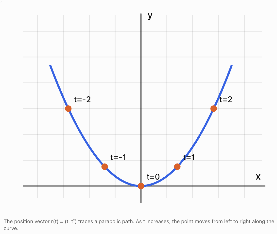
A vector-valued function describes both the shape of the path and the position of the object at each time.
This is an important distinction.
The equation y = x² describes the curve itself, while r(t) = (t, t²) also describes how the object moves along it as t changes.
Differentiating Vector-Valued Functions
Differentiation measures instantaneous rates of change.
For a scalar function:
For a vector-valued function, we differentiate each component separately.
If:
then:
The derivative is itself a vector.
Worked Example 2: Differentiating a Vector Function
Given:
Differentiate each component.
For the x-component:
For the y-component:
Therefore:
At t = 1:
This derivative describes the instantaneous rate of change of the position vector at t = 1.
Position, Velocity, and Acceleration
One of the most important applications of vector calculus is the study of motion.
Position Vector
The position vector describes where an object is located relative to an origin.
Velocity Vector
Velocity is the rate of change of position.
Therefore:
Velocity includes both magnitude and direction.
Acceleration Vector
Acceleration is the rate of change of velocity.
Therefore:
These relationships are fundamental in mechanics.
Position
\(\mathbf r(t)\)metres (m)
Velocity
\(\mathbf v(t)\)m/s
Acceleration
\(\mathbf a(t)\)m/s²
Differentiate to move from position to velocity to acceleration.
Worked Example 3: Position, Velocity, and Acceleration
A particle moves according to:
Find:
a) The velocity vector.
b) The acceleration vector.
c) The velocity and acceleration at t = 2 s.
Part a: Velocity
Differentiate position:
Part b: Acceleration
Differentiate velocity:
Part c: At t = 2
Velocity:
Acceleration:
The particle has a velocity directed right and upward, and its acceleration also has positive horizontal and vertical components.
Speed and the Magnitude of Velocity
Velocity is a vector, while speed is a scalar.
Speed is the magnitude of the velocity vector.
For two-dimensional motion:
For three-dimensional motion:
Worked Example 4: Calculating Speed
A particle has velocity:
Calculate its speed.
The speed is 10 m/s.
The direction of motion can also be calculated:
Therefore, the particle moves at 10 m/s, approximately 53.1° above the positive x-axis.
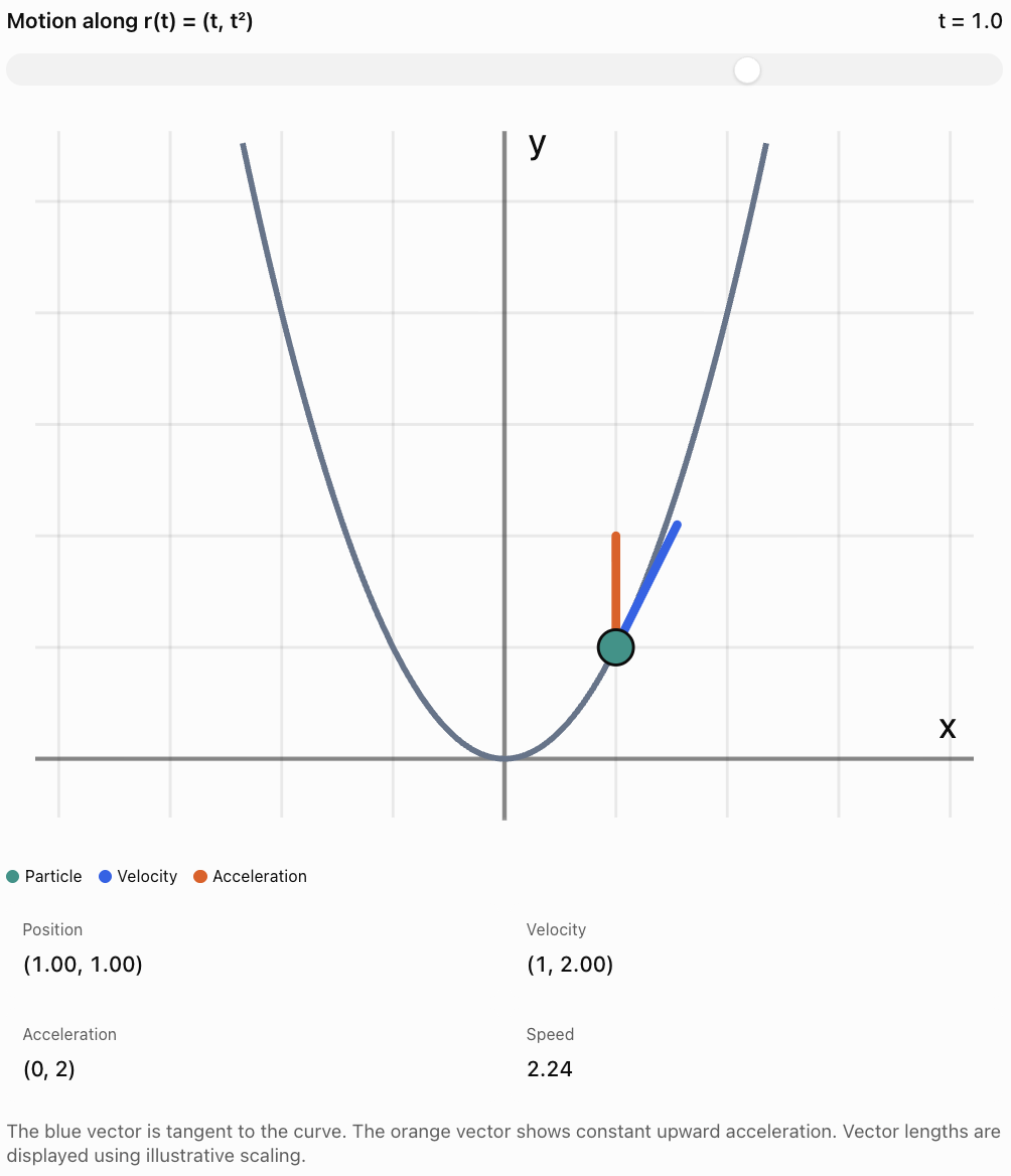
Velocity Is Tangent to the Path
The velocity vector points in the instantaneous direction of motion.
Geometrically, it is tangent to the curve traced by the position vector, provided the velocity is nonzero.
Consider:
Differentiate:
At t = 1:
The particle is at (1, 1), and its velocity points in the direction (1, 2).
This agrees with the gradient of the curve y = x² at x = 1:
The velocity vector has gradient:
The results agree.
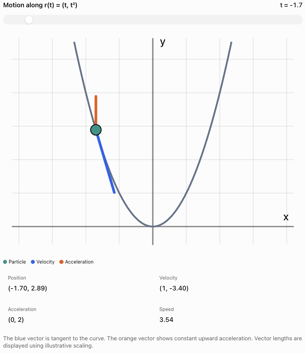
Interactive Vector Motion Explorer
Adjust time to see how a particle's position, velocity, and acceleration change along a parabolic path.
Integrating Vector-Valued Functions
Integration reverses differentiation.
If velocity is known, integration can be used to find position.
If acceleration is known, integration can be used to find velocity.
A vector-valued function is integrated component by component.
If:
then:
Here, C is a constant vector.
For motion:
with the constant vector determined by the initial position.
Similarly:
with the constant vector determined by the initial velocity.
Worked Example 5: Finding Position from Velocity
A particle has velocity:
Its initial position is:
Find its position function.
Step 1: Integrate the x-component.
Step 2: Integrate the y-component.
Therefore:
Step 3: Use the initial position.
At t = 0:
Since:
we obtain:
C₁ = 3
C₂ = −1
Therefore:
Definite Integrals and Displacement
The definite integral of velocity gives displacement.
Displacement is the change in position:
Worked Example 6: Calculating Displacement
A particle has velocity:
Calculate its displacement from t = 1 s to t = 3 s.
Integrate:
Evaluate:
x-displacement:
3² − 1² = 8
y-displacement:
3³ − 1³ = 26
Therefore:
The magnitude of the displacement is:
This is the straight-line distance between the initial and final positions, not necessarily the total distance travelled along the path.
Distance Travelled and Arc Length
Displacement and distance travelled are different quantities.
Displacement depends only on the initial and final positions.
Distance travelled measures the total length of the path.
For a vector-valued position function:
the total distance travelled from t = a to t = b is:
In three dimensions:
This is also called the arc length of the path.
Worked Example 7: Distance Along a Straight Path
A particle has velocity:
for 0 ≤ t ≤ 5.
Calculate the total distance travelled.
First find the speed:
Then:
Because the velocity is constant, the particle travels in a straight line without changing direction.
Its displacement magnitude is also 25 m.
For curved motion, the total distance travelled is generally greater than the displacement magnitude.
Projectile Motion Using Vectors
Projectile motion is an important application of vector calculus.
When air resistance is neglected, a projectile experiences constant downward acceleration due to gravity.
Taking upward as positive:
where g ≈ 9.81 m/s² near Earth's surface.
Integrating acceleration gives velocity:
Integrating velocity gives position:
For a projectile launched with speed u at angle θ above the horizontal:
v₀ₓ = u cos θ
v₀ᵧ = u sin θ
Therefore:
Worked Example 8: Projectile Motion
A ball is launched from ground level with initial speed 20 m/s at 30° above the horizontal.
Ignore air resistance.
Find:
a) The position vector after 2 s.
b) The velocity vector after 2 s.
c) The speed after 2 s.
Use g = 9.81 m/s².
Part a: Position
Horizontal initial velocity:
Vertical initial velocity:
Horizontal position after 2 s:
x = 17.32(2)
x ≈ 34.64 m
Vertical position:
y = 20 − 19.62
y = 0.38 m
Therefore:
Part b: Velocity
Horizontal velocity remains constant:
vₓ = 17.32 m/s
Vertical velocity:
vᵧ = −9.62 m/s
Therefore:
The ball is moving rightward and downward.
Part c: Speed
The speed is approximately 19.8 m/s.
Circular Motion Using Vector Functions
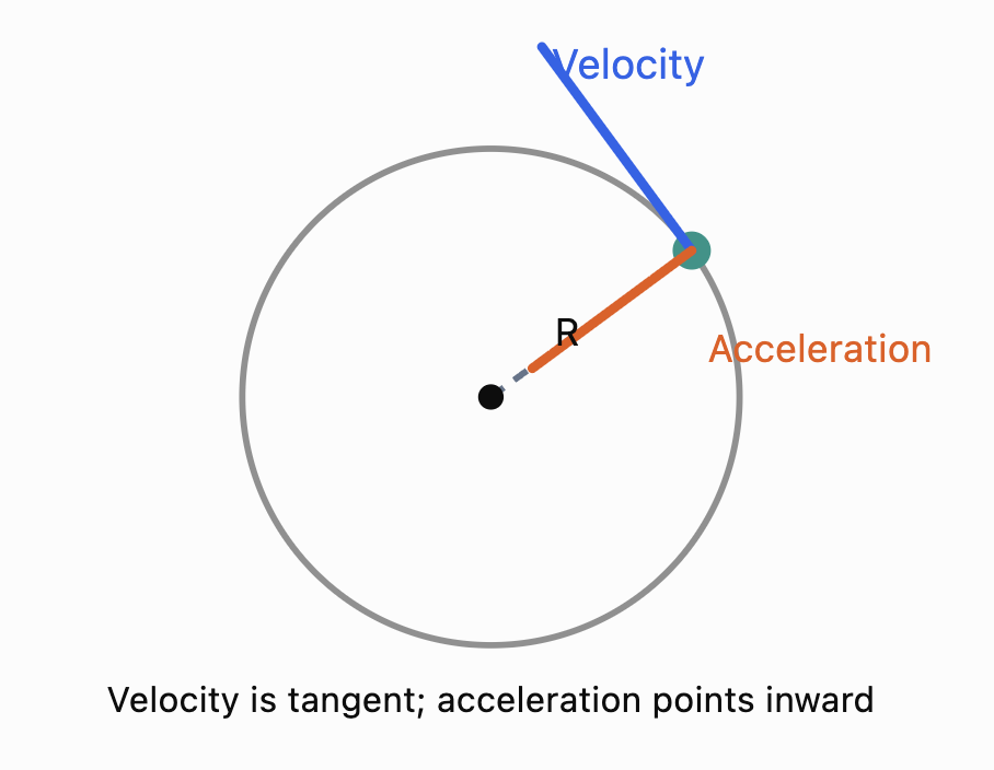
Vectors are especially important in circular motion because the direction of velocity continuously changes.
Consider an object moving around a circle of radius R with constant angular speed ω.
Its position vector is:
Differentiate to find velocity:
Differentiate again:
Notice:
The acceleration points in the opposite direction to the position vector.
Therefore, it points toward the centre of the circle.
This is centripetal acceleration.
Its magnitude is:
Worked Example 9: Circular Motion
An object moves in a circle of radius 5 m with angular speed 2 rad/s.
Calculate:
a) Its speed.
b) Its centripetal acceleration.
Part a: Speed
Part b: Centripetal acceleration
Even though the speed is constant, the object accelerates because its direction changes continuously.
The Unit Tangent Vector
The velocity vector points in the direction of motion.
To describe direction without including speed, we use the unit tangent vector.
This vector has magnitude 1.
Worked Example 10: Unit Tangent Vector
Suppose:
Then:
Its magnitude is:
Therefore:
The unit tangent vector describes the direction of motion independently of speed.
Tangential and Normal Acceleration
Acceleration can change an object's speed, direction, or both.
It is useful to divide acceleration into two components:
-
Tangential acceleration: changes speed.
-
Normal acceleration: changes direction.
For a particle moving along a smooth curve:
where:
-
T is the unit tangent vector.
-
N is the principal unit normal vector, when defined.
-
a_T is tangential acceleration.
-
a_N is normal acceleration.
The tangential component is:
The normal component is related to curvature:
where R_c is the local radius of curvature.
For circular motion, R_c is the radius of the circle.
This decomposition is useful in vehicle dynamics, roller-coaster design, aerospace engineering, and robotics.
Connecting Vectors to Multivariable Calculus
So far, we have studied vector-valued functions that depend on one variable, usually time.
Multivariable calculus studies functions that depend on two or more independent variables.
For example:
This function assigns a scalar value to each point (x, y).
It can represent a surface in three-dimensional space:
Partial Derivatives
A partial derivative measures how a multivariable function changes with respect to one variable while holding the others constant.
For:
The partial derivative with respect to x is:
The partial derivative with respect to y is:
These describe how the surface changes in the x- and y-directions.
The Gradient Vector
The gradient combines the partial derivatives of a scalar function into a vector.
For:
the gradient is:
For three variables:
The gradient points in the direction of greatest local increase of the function.
Its magnitude gives the maximum rate of increase per unit distance.
Worked Example 11: Calculating a Gradient
Given:
Find the gradient at (1, 2).
Step 1: Differentiate with respect to x.
Step 2: Differentiate with respect to y.
Therefore:
At (1, 2):
x-component:
6(1) + 2(2) = 10
y-component:
2(1) + 2(2) = 6
Therefore:
The function increases most rapidly in the direction (10, 6) at this point.
Directional Derivatives
The gradient tells us the direction of greatest increase, but what if we want the rate of change in another direction?
This is measured using a directional derivative.
For a unit vector u:
The dot product determines the rate of change in the chosen direction.
Worked Example 12: Directional Derivative
Suppose:
We want the rate of change in the direction:
Calculate:
The function increases at a rate of 10 units per unit distance in the specified direction.
Vector Fields
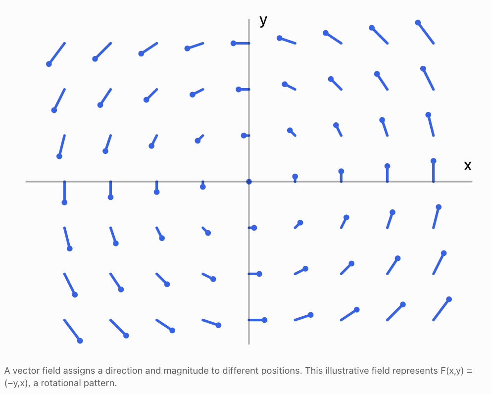
A vector field assigns a vector to every point in a region.
For example, a wind field may describe the velocity of air at different locations.
Possible vector fields include:
-
Wind velocity.
-
Water flow.
-
Gravitational fields.
-
Electric fields.
-
Magnetic fields.
-
Force fields.
Worked Example 13: Evaluating a Vector Field
Suppose:
\[ \mathbf F(x,y)=2x\mathbf i-3y\mathbf j \]Find the vector at (2, −1).
Substitute:
\[ \mathbf F(2,-1)=2(2)\mathbf i-3(-1)\mathbf j \]Therefore:
\[ \boxed{\mathbf F(2,-1)=4\mathbf i+3\mathbf j} \]The vector points right and upward.
Its magnitude is:
\[ |\mathbf F|=\sqrt{4^2+3^2}=5 \]The Chain Rule for Motion Through a Scalar Field
Vector calculus also connects motion to changing physical conditions.
Suppose the temperature in a room depends on position:
T = T(x, y)
A moving sensor follows a path:
\[ \mathbf r(t)=x(t)\mathbf i+y(t)\mathbf j \]The temperature experienced by the sensor changes as it moves.
The multivariable chain rule gives:
\[ \boxed{ \frac{dT}{dt}= \frac{\partial T}{\partial x}\frac{dx}{dt}+ \frac{\partial T}{\partial y}\frac{dy}{dt} } \]In vector form:
\[ \boxed{\frac{dT}{dt}=\nabla T\cdot\mathbf v} \]This formula connects the temperature gradient with the sensor's velocity.
Worked Example 14: Moving Through a Temperature Field
Suppose:
\[ T(x,y)=20+2x+3y \]A sensor moves with velocity:
\[ \mathbf v=4\mathbf i+\mathbf j\text{ m/s} \]Find the rate of change of temperature experienced by the sensor.
First calculate the gradient:
\[ \nabla T=2\mathbf i+3\mathbf j \]Then:
\[ \frac{dT}{dt}=\nabla T\cdot\mathbf v \]\[ =2(4)+3(1) \]\[ \boxed{\frac{dT}{dt}=11^\circ\text{C/s}} \]The sensor experiences a temperature increase of 11°C per second under this idealised model.
This type of calculation is useful in environmental science, fluid dynamics, and heat transfer.
The Jacobian Matrix
For functions with several inputs and several outputs, derivatives can be organised into a matrix called the Jacobian.
Suppose:
\[ \mathbf F(x,y)= \begin{bmatrix} f(x,y)\\ g(x,y) \end{bmatrix} \]The Jacobian matrix is:
\[ \boxed{ J= \begin{bmatrix} \frac{\partial f}{\partial x}&\frac{\partial f}{\partial y}\\ \frac{\partial g}{\partial x}&\frac{\partial g}{\partial y} \end{bmatrix} } \]The Jacobian describes how small changes in the inputs affect the outputs.
Worked Example 15: Calculating a Jacobian
Given:
\[ \mathbf F(x,y)= \begin{bmatrix} x^2+y\\ xy \end{bmatrix} \]Calculate the Jacobian.
For the first component:
f(x, y) = x² + y
\[ \frac{\partial f}{\partial x}=2x \]\[ \frac{\partial f}{\partial y}=1 \]For the second component:
g(x, y) = xy
\[ \frac{\partial g}{\partial x}=y \]\[ \frac{\partial g}{\partial y}=x \]Therefore:
\[ \boxed{ J(x,y)= \begin{bmatrix} 2x&1\\ y&x \end{bmatrix} } \]At (2, 3):
\[ \boxed{ J(2,3)= \begin{bmatrix} 4&1\\ 3&2 \end{bmatrix} } \]The Jacobian is widely used in robotics, optimisation, coordinate transformations, and numerical methods.
Real-World Applications of Vector Calculus
Orbital Mechanics
Vector functions describe the positions and velocities of satellites and spacecraft. Differentiation determines velocity and acceleration, while integration predicts future motion from known forces.
Fluid Dynamics
Engineers model air and water movement using vector fields. Velocity, acceleration, pressure gradients, and fluid-flow rates are analysed using vector calculus.
Robotics
Vector-valued functions describe robot trajectories. Derivatives determine tool velocities and accelerations, while Jacobian matrices connect joint movement to end-effector motion.
Meteorology
Wind velocity is a vector field. Weather models use spatial derivatives and time-dependent equations to describe changes in atmospheric conditions.
Electromagnetism
Electric and magnetic fields are vector fields. Advanced vector calculus describes how these fields vary through space and time.
Common Mistakes
Mistake 1: Differentiating the magnitude instead of the vector components
Differentiate each component of the vector-valued function separately.
Mistake 2: Confusing speed and velocity
Speed is a scalar. Velocity is a vector containing magnitude and direction.
Mistake 3: Assuming constant speed means zero acceleration
An object moving in a circle at constant speed still accelerates because its direction changes.
Mistake 4: Forgetting the constant vector when integrating
Each component may have its own integration constant. Together, these form a constant vector.
Mistake 5: Confusing displacement with distance travelled
Displacement is the change in position. Distance travelled is the length of the path.
Mistake 6: Assuming velocity and acceleration always point in the same direction
Acceleration may point in a different direction from velocity.
Mistake 7: Forgetting units
Position is measured in metres, velocity in m/s, and acceleration in m/s².
Mistake 8: Confusing scalar functions and vector-valued functions
A scalar function produces a number. A vector-valued function produces a vector.
Mistake 9: Treating the gradient as a scalar
The gradient is a vector composed of partial derivatives.
Mistake 10: Forgetting to use a unit vector in directional derivatives
The formula Dᵤf = ∇f · u assumes u has magnitude 1.
Mistake 11: Confusing partial derivatives with ordinary derivatives
A partial derivative varies one independent variable while holding the others fixed.
Mistake 12: Assuming a mathematical model always describes physical reality perfectly
Vector models may neglect friction, air resistance, changing forces, and other real-world effects.
Key Terms
-
Vector-Valued Function: Function that produces a vector as its output.
-
Position Vector: Vector describing an object's position relative to an origin.
-
Velocity Vector: Rate of change of position with respect to time.
-
Acceleration Vector: Rate of change of velocity with respect to time.
-
Speed: Magnitude of the velocity vector.
-
Vector Derivative: Derivative obtained by differentiating vector components.
-
Vector Integral: Integral obtained by integrating vector components.
-
Displacement: Change in position between two points.
-
Distance Travelled: Total length of the path followed.
-
Arc Length: Length of a curve over a specified interval.
-
Parametric Curve: Curve described by coordinate functions of a parameter.
-
Tangent Vector: Vector pointing along a curve.
-
Unit Tangent Vector: Tangent vector with magnitude 1.
-
Normal Vector: Vector perpendicular to the tangent direction.
-
Tangential Acceleration: Component of acceleration that changes speed.
-
Normal Acceleration: Component of acceleration that changes direction.
-
Centripetal Acceleration: Acceleration directed toward the centre of circular motion.
-
Angular Speed: Rate of change of angular position.
-
Scalar Field: Function assigning a scalar to every point in a region.
-
Vector Field: Function assigning a vector to every point in a region.
-
Partial Derivative: Derivative with respect to one variable while others remain fixed.
-
Gradient: Vector containing the partial derivatives of a scalar field.
-
Directional Derivative: Rate of change of a scalar function in a specified direction.
-
Multivariable Chain Rule: Rule for differentiating a function that depends on several changing variables.
-
Jacobian Matrix: Matrix of first-order partial derivatives of a vector-valued function.
-
Curvature: Measure of how sharply a curve changes direction.
-
Line Integral: Integral evaluated along a curve.
-
Vector Calculus: Branch of mathematics combining vector methods with differentiation and integration.
Key Takeaways
-
Vector-valued functions describe positions and other vector quantities that change with a parameter.
-
A position vector can describe motion along a curve in two or three dimensions.
-
Differentiating position gives velocity.
-
Differentiating velocity gives acceleration.
-
Speed is the magnitude of velocity.
-
Velocity is tangent to the path of motion when it is nonzero.
-
Integrating acceleration gives velocity, subject to an initial velocity.
-
Integrating velocity gives position, subject to an initial position.
-
Definite integration of velocity gives displacement.
-
Integrating speed gives total distance travelled.
-
Circular motion can involve constant speed but nonzero acceleration.
-
The gradient describes the direction and rate of greatest local increase of a scalar field.
-
Directional derivatives measure change in specified directions.
-
Vector fields describe quantities such as wind velocity, fluid flow, and electromagnetic fields.
-
Jacobian matrices connect vector functions to multivariable differentiation.
-
Vector calculus is essential in physics, engineering, robotics, and scientific modelling.
Check Your Understanding
Questions
Question 1: Vector-Valued Functions
Given:
\[ \mathbf r(t)=(3t+2)\mathbf i+(t^2-1)\mathbf j \]Find the position at t = 2.
Question 2: Vector Differentiation
Differentiate:
\[ \mathbf r(t)=t^3\mathbf i+(4t^2-3t)\mathbf j \]Question 3: Velocity and Acceleration
A particle moves according to:
\[ \mathbf r(t)=2t^2\mathbf i+(t^3-2t)\mathbf j \]Find its velocity and acceleration functions.
Question 4: Instantaneous Velocity
For the particle in Question 3, calculate the velocity at t = 2 s.
Question 5: Speed
A particle has velocity:
\[ \mathbf v=5\mathbf i+12\mathbf j \]Calculate its speed.
Question 6: Vector Integration
Integrate:
\[ \mathbf v(t)=6t\mathbf i+4t^3\mathbf j \]Question 7: Initial Conditions
A particle has velocity:
\[ \mathbf v(t)=2t\mathbf i+3\mathbf j \]Its initial position is:
\[ \mathbf r(0)=4\mathbf i-2\mathbf j \]Find its position function.
Question 8: Displacement
A particle has velocity:
\[ \mathbf v(t)=4t\mathbf i+2\mathbf j \]Calculate its displacement from t = 0 to t = 3.
Question 9: Circular Motion
An object moves in a circle of radius 4 m with angular speed 3 rad/s.
Calculate its speed and centripetal acceleration.
Question 10: Unit Tangent Vector
Given:
\[ \mathbf v=8\mathbf i+6\mathbf j \]Find the unit tangent vector.
Question 11: Partial Derivatives
Given:
\[ f(x,y)=4x^2+3xy+y^2 \]Find both first-order partial derivatives.
Question 12: Gradient
For the function in Question 11, calculate the gradient at (1, 2).
Question 13: Directional Derivative
A scalar field has gradient:
\[ \nabla f=3\mathbf i+4\mathbf j \]Calculate the directional derivative in the direction:
\[ \mathbf u=\frac35\mathbf i+\frac45\mathbf j \]Question 14: Vector Field
Given:
\[ \mathbf F(x,y)=x^2\mathbf i+2y\mathbf j \]Calculate the field vector at (2, −3).
Question 15: Integrated Motion Problem
A particle moves according to:
\[ \mathbf r(t)=(t^3-3t)\mathbf i+(2t^2+1)\mathbf j \]a) Find the velocity vector.
b) Find the acceleration vector.
c) Calculate the position at t = 2.
d) Calculate the velocity at t = 2.
e) Calculate the speed at t = 2.
f) Calculate the displacement from t = 0 to t = 2.
g) Explain the difference between the displacement magnitude and total distance travelled.
Fully Worked Answers
Answer 1: Vector-Valued Functions
Given:
\[ \mathbf r(t)=(3t+2)\mathbf i+(t^2-1)\mathbf j \]At t = 2:
x = 3(2) + 2 = 8
y = 2² − 1 = 3
Therefore:
\[ \boxed{\mathbf r(2)=8\mathbf i+3\mathbf j} \]Answer 2: Vector Differentiation
Differentiate each component:
\[ \frac{d}{dt}(t^3)=3t^2 \]\[ \frac{d}{dt}(4t^2-3t)=8t-3 \]Therefore:
\[ \boxed{\mathbf r'(t)=3t^2\mathbf i+(8t-3)\mathbf j} \]Answer 3: Velocity and Acceleration
Given:
\[ \mathbf r(t)=2t^2\mathbf i+(t^3-2t)\mathbf j \]Differentiate:
\[ \boxed{\mathbf v(t)=4t\mathbf i+(3t^2-2)\mathbf j} \]Differentiate again:
\[ \boxed{\mathbf a(t)=4\mathbf i+6t\mathbf j} \]Answer 4: Instantaneous Velocity
From Question 3:
\[ \mathbf v(t)=4t\mathbf i+(3t^2-2)\mathbf j \]At t = 2:
x-component:
4(2) = 8
y-component:
3(2²) − 2 = 10
Therefore:
\[ \boxed{\mathbf v(2)=8\mathbf i+10\mathbf j\text{ m/s}} \]Answer 5: Speed
\[ \mathbf v=5\mathbf i+12\mathbf j \]\[ |\mathbf v|=\sqrt{5^2+12^2} \]\[ =\sqrt{25+144} \]\[ =\sqrt{169} \]\[ \boxed{|\mathbf v|=13} \]If velocity is measured in m/s, the speed is 13 m/s.
Answer 6: Vector Integration
\[ \mathbf v(t)=6t\mathbf i+4t^3\mathbf j \]Integrate each component:
\[ \int6t\,dt=3t^2+C_1 \]\[ \int4t^3\,dt=t^4+C_2 \]Therefore:
\[ \boxed{\mathbf r(t)=3t^2\mathbf i+t^4\mathbf j+\mathbf C} \]where C is a constant vector.
Answer 7: Initial Conditions
Given:
\[ \mathbf v(t)=2t\mathbf i+3\mathbf j \]Integrate:
\[ \mathbf r(t)=(t^2+C_1)\mathbf i+(3t+C_2)\mathbf j \]Initial position:
\[ \mathbf r(0)=4\mathbf i-2\mathbf j \]Therefore:
C₁ = 4
C₂ = −2
Hence:
\[ \boxed{\mathbf r(t)=(t^2+4)\mathbf i+(3t-2)\mathbf j} \]Answer 8: Displacement
\[ \Delta\mathbf r=\int_0^3(4t\mathbf i+2\mathbf j)\,dt \]Integrate:
\[ \Delta\mathbf r=[2t^2]_0^3\mathbf i+[2t]_0^3\mathbf j \]x-displacement:
2(3²) = 18
y-displacement:
2(3) = 6
Therefore:
\[ \boxed{\Delta\mathbf r=18\mathbf i+6\mathbf j} \]Answer 9: Circular Motion
Given:
R = 4 m
ω = 3 rad/s
Speed:
\[ v=R\omega \]\[ v=4(3) \]\[ \boxed{v=12\text{ m/s}} \]Centripetal acceleration:
\[ a_c=R\omega^2 \]\[ a_c=4(3)^2 \]\[ \boxed{a_c=36\text{ m/s}^2} \]Answer 10: Unit Tangent Vector
Given:
\[ \mathbf v=8\mathbf i+6\mathbf j \]Magnitude:
\[ |\mathbf v|=\sqrt{8^2+6^2}=10 \]Therefore:
\[ \mathbf T=\frac{\mathbf v}{|\mathbf v|} \]\[ \boxed{\mathbf T=\frac45\mathbf i+\frac35\mathbf j} \]Answer 11: Partial Derivatives
Given:
\[ f(x,y)=4x^2+3xy+y^2 \]Differentiate with respect to x:
\[ \boxed{\frac{\partial f}{\partial x}=8x+3y} \]Differentiate with respect to y:
\[ \boxed{\frac{\partial f}{\partial y}=3x+2y} \]Answer 12: Gradient
The gradient is:
\[ \nabla f=(8x+3y)\mathbf i+(3x+2y)\mathbf j \]At (1, 2):
x-component:
8(1) + 3(2) = 14
y-component:
3(1) + 2(2) = 7
Therefore:
\[ \boxed{\nabla f(1,2)=14\mathbf i+7\mathbf j} \]Answer 13: Directional Derivative
Given:
\[ \nabla f=3\mathbf i+4\mathbf j \]and:
\[ \mathbf u=\frac35\mathbf i+\frac45\mathbf j \]Calculate:
\[ D_{\mathbf u}f=\nabla f\cdot\mathbf u \]\[ =3\left(\frac35\right)+4\left(\frac45\right) \]\[ =\frac95+\frac{16}{5} \]\[ =\frac{25}{5} \]\[ \boxed{D_{\mathbf u}f=5} \]Answer 14: Vector Field
Given:
\[ \mathbf F(x,y)=x^2\mathbf i+2y\mathbf j \]At (2, −3):
x-component:
2² = 4
y-component:
2(−3) = −6
Therefore:
\[ \boxed{\mathbf F(2,-3)=4\mathbf i-6\mathbf j} \]Answer 15: Integrated Motion Problem
Given:
\[ \mathbf r(t)=(t^3-3t)\mathbf i+(2t^2+1)\mathbf j \]Part a: Velocity
Differentiate:
\[ \boxed{\mathbf v(t)=(3t^2-3)\mathbf i+4t\mathbf j} \]Part b: Acceleration
Differentiate velocity:
\[ \boxed{\mathbf a(t)=6t\mathbf i+4\mathbf j} \]Part c: Position at t = 2
x-component:
2³ − 3(2) = 8 − 6 = 2
y-component:
2(2²) + 1 = 9
Therefore:
\[ \boxed{\mathbf r(2)=2\mathbf i+9\mathbf j} \]Part d: Velocity at t = 2
x-component:
3(2²) − 3 = 9
y-component:
4(2) = 8
Therefore:
\[ \boxed{\mathbf v(2)=9\mathbf i+8\mathbf j} \]Part e: Speed at t = 2
\[ |\mathbf v(2)|=\sqrt{9^2+8^2} \]\[ =\sqrt{145} \]\[ \boxed{|\mathbf v(2)|\approx12.04} \]Part f: Displacement from t = 0 to t = 2
Initial position:
\[ \mathbf r(0)=0\mathbf i+1\mathbf j \]Final position:
\[ \mathbf r(2)=2\mathbf i+9\mathbf j \]Therefore:
\[ \Delta\mathbf r=\mathbf r(2)-\mathbf r(0) \]\[ \boxed{\Delta\mathbf r=2\mathbf i+8\mathbf j} \]Magnitude:
\[ |\Delta\mathbf r|=\sqrt{2^2+8^2} \]\[ =\sqrt{68} \]\[ \boxed{|\Delta\mathbf r|\approx8.25} \]Part g: Displacement versus distance
The displacement magnitude is approximately 8.25 units.
However, the particle follows a curved path, so the total distance travelled is greater than the straight-line displacement.
The distance travelled would be calculated using:
\[ s=\int_0^2|\mathbf v(t)|\,dt \]Therefore:
\[ \boxed{ s=\int_0^2\sqrt{(3t^2-3)^2+(4t)^2}\,dt } \]This integral gives the total arc length of the path and can be evaluated numerically.
Final Reflection
Vector calculus extends ordinary differentiation and integration into two and three dimensions.
Vector-valued functions allow us to describe motion along curved paths. Differentiation gives velocity and acceleration, while integration allows us to calculate displacement and recover position from known motion.
The geometric interpretation is equally important. Velocity is tangent to the path, while acceleration may change speed, direction, or both. Circular motion provides a clear example of acceleration occurring even when speed remains constant.
Vector calculus also provides the foundation for multivariable mathematics. Gradients, directional derivatives, vector fields, and Jacobian matrices allow scientists to investigate how quantities change across space.
These ideas are essential in physics, engineering, robotics, fluid dynamics, meteorology, electromagnetism, and many other fields.
The central idea is that vector calculus combines magnitude, direction, and rates of change to describe and analyse motion and physical systems in multiple dimensions.
-
2. Linear Algebra Foundations
Learning outcomes
- I can explain the role of vectors and matrices in linear algebra.
- I can identify vector spaces conceptually.
- I can recognise linear independence.
- I can interpret basis vectors.
- I can appreciate the foundations of higher mathematics.
Introduction
Linear algebra is one of the most important branches of modern mathematics. It provides the mathematical foundation for studying vectors, matrices, systems of equations, transformations, and relationships between quantities.
Many mathematical ideas that initially appear unrelated are connected through linear algebra.
For example:
-
A system of simultaneous equations can be represented by a matrix.
-
A geometric transformation can be described using matrix multiplication.
-
A collection of vectors can describe an entire space.
-
A small number of basis vectors can represent infinitely many other vectors.
-
Linear independence helps determine whether mathematical information is redundant.
-
Eigenvalues and eigenvectors reveal important properties of transformations and dynamic systems.
Linear algebra is essential in physics, engineering, computer science, economics, statistics, artificial intelligence, and advanced mathematics.
The central idea is that complicated mathematical structures can often be understood by studying combinations of vectors and the transformations that act on them.
What Is Linear Algebra?
Linear algebra is the branch of mathematics concerned with vectors, vector spaces, linear transformations, matrices, and systems of linear equations.
A relationship is linear when it preserves addition and scalar multiplication in the appropriate mathematical setting.
For example, the equation:
2x + 3y = 12
is a linear equation in two variables.
The system:
2x + 3y = 12
4x − y = 5
can be written as:
Or more simply:
where:
-
A is a matrix of coefficients.
-
x is a vector of unknown quantities.
-
b is a vector of known values.
This equation is one of the fundamental structures of linear algebra.
It appears in scientific modelling, engineering, data analysis, optimisation, and computer simulations.
The Role of Vectors in Linear Algebra
A vector is an object that can be added to another vector and multiplied by a scalar.
In elementary mathematics, vectors are commonly represented as arrows with magnitude and direction.
For example:
This vector represents a displacement of:
-
3 units in the positive x-direction.
-
4 units in the positive y-direction.
Its magnitude is:
However, linear algebra uses a broader understanding of vectors.
Vectors can also represent:
-
Lists of measurements.
-
Forces acting on objects.
-
Electrical currents.
-
Coefficients of polynomials.
-
Images represented by pixel values.
-
Data describing populations.
-
Signals and functions.
The important feature is not necessarily the arrow representation, but the mathematical rules governing vector addition and scalar multiplication.
Vector Addition
Given:
Add corresponding components:
Scalar Multiplication
Multiplying a vector by a scalar changes its magnitude and possibly its direction.
For:
Multiplying by 4 gives:
Multiplying by −1 gives:
The negative scalar reverses the direction of the vector.
These two operations form the basis of vector spaces.
Linear Combinations of Vectors
A linear combination is an expression formed by multiplying vectors by scalars and adding the results.
For two vectors:
where a and b are scalars.
For several vectors:
Linear combinations are fundamental because they allow us to construct new vectors from existing ones.
Worked Example 1: Finding a Linear Combination
Given:
Find:
2u − 3v
First calculate:
Then:
Subtract:
Therefore:
Worked Example 2: Expressing a Vector as a Linear Combination
Given:
Express:
as a linear combination of u and v.
We want:
Therefore:
This produces:
a + b = 6
a − b = 2
Add the equations:
2a = 8
a = 4
Substitute:
4 + b = 6
b = 2
Therefore:
This demonstrates how one vector can be constructed from other vectors.
What Is a Vector Space?
A vector space is a collection of objects called vectors that can be added together and multiplied by scalars while satisfying specific mathematical rules.
For this lesson, we will focus on vector spaces over the real numbers.
A vector space must be closed under two operations:
-
Vector addition.
-
Scalar multiplication.
Closure under addition means that adding two vectors from the space produces another vector in the same space.
Closure under scalar multiplication means that multiplying a vector from the space by any real scalar produces another vector in the same space.
A vector space must also satisfy additional rules, including the existence of a zero vector, additive inverses, and the usual associative and distributive properties.
Example 1: Two-Dimensional Space
The set of all ordered pairs of real numbers is written:
A typical vector is:
where x and y are real numbers.
Examples include:
(2, 3)
(−1, 5)
(0, 0)
(π, √2)
All such vectors belong to ℝ².
If two vectors in ℝ² are added, the result remains in ℝ².
If a vector in ℝ² is multiplied by a real number, the result remains in ℝ².
Therefore, ℝ² is a vector space.
Example 2: Three-Dimensional Space
The set:
contains all ordered triples of real numbers.
A typical vector is:
This space is used extensively in physics, engineering, and computer graphics.
Example 3: Polynomial Vector Spaces
Consider all polynomials of degree at most 2:
where a, b, and c are real numbers.
Two such polynomials can be added:
The result is another polynomial of degree at most 2.
Multiplying by a scalar also produces a polynomial of degree at most 2.
Therefore, these polynomials form a vector space.
Notice that the objects are functions rather than arrows.
This is an important example of the abstract nature of linear algebra.
Vector Spaces and Subspaces
A subspace is a smaller vector space contained within a larger vector space.
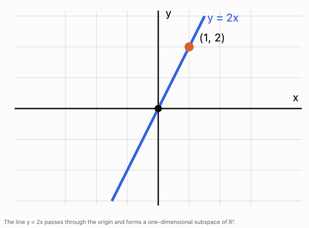
For example, consider all vectors in ℝ² that lie on the line:
y = 2x
These vectors have the form:
where t is any real number.
Equivalently:
This collection forms a subspace of ℝ².
It includes the zero vector when t = 0.
Adding two vectors on the line produces another vector on the line.
Multiplying any vector on the line by a scalar keeps it on the line.
Why Not Every Line Is a Subspace
Consider:
y = 2x + 3
This line does not pass through the origin.
The zero vector (0, 0) does not lie on the line.
Therefore, the line is not a vector subspace of ℝ².
Important principle: Every vector subspace must contain the zero vector.
The Span of a Set of Vectors
The span of a collection of vectors is the set of all possible linear combinations of those vectors.
For vectors u and v:
The span tells us what part of a vector space can be reached using the given vectors.
Example 1: One Vector in Two Dimensions
Suppose:
All scalar multiples of u lie on a line through the origin.
Therefore:
is a line.
Example 2: Two Independent Vectors in Two Dimensions
Suppose:
Any vector:
can be written as:
Therefore:
These two vectors span the entire two-dimensional plane.
Example 3: Two Vectors on the Same Line
Suppose:
Since:
the vectors point along the same line.
Their span is only a line, not the entire plane.
Adding the second vector does not create any new direction.
Linear Independence
Vectors are linearly independent when none of them can be written as a linear combination of the others.
In two dimensions, two nonzero vectors are linearly independent when they do not lie along the same line through the origin.
For example:
are independent.
Neither vector can be obtained by multiplying the other by a scalar.
However:
are dependent because:
Formal Definition
Vectors v₁, v₂, ..., vₙ are linearly independent if the equation:
has only the solution:
This is called the trivial solution.
If another solution exists in which at least one coefficient is nonzero, the vectors are linearly dependent.
Visualising Linear Independence
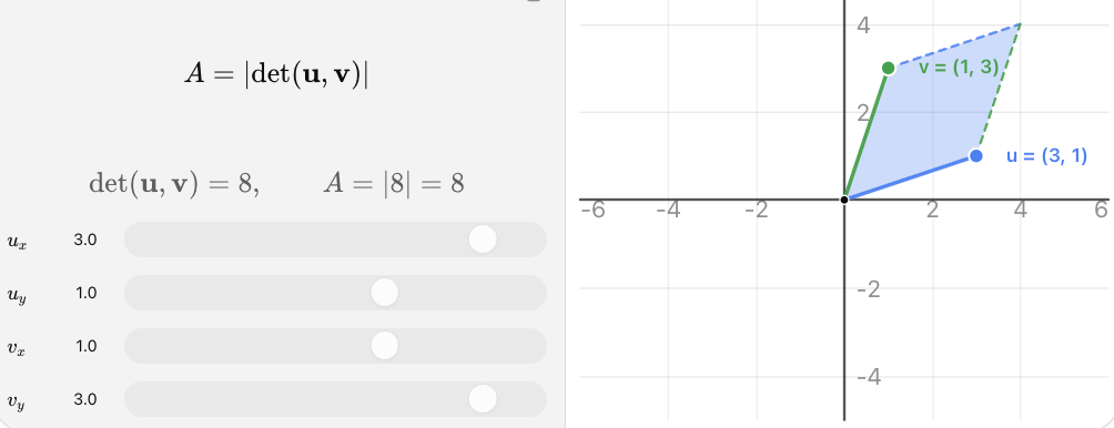
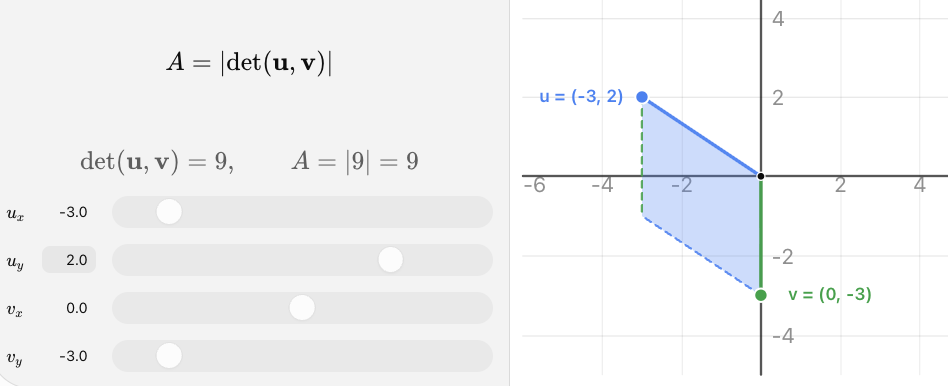
Move the vectors to investigate what happens when they point in different directions or become parallel.
When two vectors in ℝ² are independent, the parallelogram formed by them has nonzero area. When they are dependent, the parallelogram collapses into a line and its area becomes zero.
Worked Example 3: Testing Independence Using a Determinant
Given:
Construct a matrix using the vectors as columns:
Calculate its determinant:
Since the determinant is not zero, the vectors are linearly independent.
Worked Example 4: Identifying Dependent Vectors
Given:
Notice:
Therefore, the vectors are linearly dependent.
We can also check using the determinant:
The zero determinant confirms that the vectors are dependent.
Important: The determinant test applies directly when the vectors form a square matrix, such as two vectors in ℝ² or three vectors in ℝ³. More general collections can be tested using row reduction or the defining equation for linear independence.
Linear Independence in Three Dimensions
In ℝ³, three vectors are linearly independent when none can be expressed as a linear combination of the other two.
For example, the vectors:
are linearly independent.
They point along three distinct coordinate directions.
Together, they span all of ℝ³.
Any vector:
can be expressed as:
However, three vectors that all lie in the same plane through the origin cannot span ℝ³.
They do not provide three independent directions.
Basis Vectors
A basis is a set of vectors that satisfies two conditions:
-
The vectors are linearly independent.
-
The vectors span the entire vector space.
A basis provides a set of fundamental directions from which every vector in the space can be constructed.
The Standard Basis of ℝ²
The standard basis vectors are:
Any vector:
can be written as:
For example:
The Standard Basis of ℝ³
The standard basis is:
Any vector in ℝ³ can be expressed as a linear combination of these three basis vectors.
A Vector Space Can Have Different Bases
The standard basis is not the only possible basis.
For example, consider:
These vectors are linearly independent because:
Since the determinant is nonzero, they form a basis for ℝ².
Worked Example 5: Coordinates in a Different Basis
Express:
using the basis:
We want:
This gives:
a + b = 8
a − b = 2
Add:
2a = 10
a = 5
Then:
b = 3
Therefore:
The coordinates of w in the basis B are:
The vector itself has not changed.
Only the coordinate system used to describe it has changed.
This distinction is important in advanced mathematics, physics, and engineering.
Dimension of a Vector Space
The dimension of a finite-dimensional vector space is the number of vectors in any basis for that space.
Examples:
|
Vector space |
Dimension |
Example basis |
|---|---|---|
|
ℝ¹ |
1 |
(1) |
|
ℝ² |
2 |
(1, 0), (0, 1) |
|
ℝ³ |
3 |
(1, 0, 0), (0, 1, 0), (0, 0, 1) |
|
Polynomials of degree at most 2 |
3 |
1, x, x² |
|
2 × 2 real matrices |
4 |
Four matrices each with one entry equal to 1 and all others 0 |
Why Dimension Matters
Dimension tells us how many independent quantities are needed to describe an object in the space.
For example:
-
A point on a line requires one coordinate.
-
A point in a plane requires two coordinates.
-
A point in ordinary three-dimensional space requires three coordinates.
-
A quadratic polynomial requires three coefficients.
The concept extends to much larger spaces.
A digital image containing 1,000 grayscale pixels can be represented as a vector in ℝ¹⁰⁰⁰.
This is one reason linear algebra is so important in data science and artificial intelligence.
The Role of Matrices in Linear Algebra
Matrices are closely connected to vectors and vector spaces.
A matrix can represent a linear transformation.
A linear transformation is a function T satisfying:
and:
These properties mean that the transformation preserves vector addition and scalar multiplication.
Example: A Linear Transformation
Consider:
This transformation doubles the x-coordinate and triples the y-coordinate.
Its matrix is:
For:
we calculate:
Therefore:
The matrix describes how the transformation acts on vectors.
Matrix Columns and Basis Vectors
An especially important result is that the columns of a transformation matrix describe what happens to the standard basis vectors.
Consider:
Apply A to the first standard basis vector:
Apply A to the second standard basis vector:
The first column of A is the image of the first basis vector.
The second column of A is the image of the second basis vector.
Therefore:
This is a fundamental connection between matrices and linear transformations.
Once we know what a linear transformation does to every vector in a basis, we know what it does to every vector in the space.
Rank and the Number of Independent Directions
The rank of a matrix is the number of linearly independent columns, which is also equal to the number of linearly independent rows.
Rank describes how many independent directions are preserved by a linear transformation.
Worked Example 6: Determining Matrix Rank
Consider:
The second column is twice the first.
Therefore, the columns are linearly dependent.
The matrix has rank 1.
Now consider:
Its determinant is:
Since the determinant is nonzero, the columns are independent.
Therefore:
Geometric Interpretation
A rank-2 transformation in ℝ² preserves two independent directions and maps the plane onto the plane.
A rank-1 transformation in ℝ² maps every vector onto a line through the origin.
A rank-0 transformation maps every vector to the zero vector.
Rank is important when solving systems of equations and analysing datasets.
Linear Algebra and Systems of Equations
Consider:
The columns of A can be interpreted as vectors.
For example:
This means:
The question becomes:
Can the target vector be expressed as a linear combination of the columns of A?
If the columns form a basis for ℝ², every target vector in ℝ² can be represented uniquely.
If the columns are dependent, some target vectors may not be reachable, and others may have infinitely many representations.
Worked Example 7: Solving a System Using Column Vectors
Solve:
2x + y = 5
x + 3y = 7
From the first equation:
y = 5 − 2x
Substitute into the second:
x + 3(5 − 2x) = 7
x + 15 − 6x = 7
−5x = −8
Then:
Therefore:
This means:
The target vector is expressed as a linear combination of two independent column vectors.
Connections to Higher Mathematics
Linear algebra provides the foundation for many advanced mathematical ideas.
Eigenvalues and Eigenvectors
An eigenvector is a nonzero vector whose direction is preserved by a linear transformation, apart from possible reversal.
where λ is an eigenvalue.
Eigenvalues help describe the behaviour of transformations, vibrations, population models, and dynamic systems.
Differential Equations
Systems of differential equations can be written in matrix form.
For example:
Such equations describe how several quantities change together over time.
They are important in physics, engineering, biology, and economics.
Multivariable Calculus
Matrices describe derivatives of functions with multiple inputs and outputs.
The Jacobian matrix organises partial derivatives.
For:
the Jacobian is:
This connects linear algebra with calculus.
Optimisation
Many optimisation problems involve finding the best possible solution under constraints.
Linear algebra is used to represent the constraints and calculate efficient solutions.
Examples include:
-
Minimising production costs.
-
Optimising transport networks.
-
Designing efficient structures.
-
Fitting mathematical models to data.
Data Science and Machine Learning
Large datasets can be represented using matrices.
Rows may represent observations, while columns represent variables.
Linear algebra supports:
-
Linear regression.
-
Principal component analysis.
-
Neural networks.
-
Image recognition.
-
Recommendation systems.
-
Data compression.
Real-World Applications
Robotics and Engineering
Robots use vectors and matrices to represent positions, orientations, and movement. Basis changes allow engineers to convert coordinates between different reference frames.
Computer Graphics
Matrices transform three-dimensional objects through rotations, reflections, scaling, and projections. Graphics software relies on efficient matrix calculations.
Artificial Intelligence
Machine learning systems process large collections of numerical data. Matrix multiplication is a fundamental operation in neural networks and other models.
Structural Engineering
Engineers use matrix methods to calculate forces, displacements, and stresses in buildings and bridges. Rank and independence help determine whether engineering equations provide enough information.
Statistics and Scientific Research
Matrices organise measurements and support regression, covariance analysis, and dimensionality reduction. Independent variables provide distinct information about a system.
Common Mistakes
Mistake 1: Thinking vectors must always represent arrows
Vectors can also be lists of numbers, functions, polynomials, and other mathematical objects.
Mistake 2: Confusing a vector with a scalar
A scalar is a number, while a vector is an element of a vector space.
Mistake 3: Assuming any collection of vectors forms a vector space
A vector space must satisfy specific rules, including closure under addition and scalar multiplication.
Mistake 4: Forgetting the zero vector
Every vector space and subspace must contain the zero vector.
Mistake 5: Assuming every line in ℝ² is a subspace
Only lines passing through the origin are one-dimensional subspaces of ℝ².
Mistake 6: Confusing span with linear independence
Span describes the vectors that can be constructed. Independence describes whether the original vectors contain redundant information.
Mistake 7: Assuming two different vectors are always independent
Two different vectors may still be scalar multiples of one another.
Mistake 8: Confusing a basis with any collection of vectors
A basis must both span the space and be linearly independent.
Mistake 9: Assuming every basis must use standard coordinate vectors
Many different bases can describe the same vector space.
Mistake 10: Confusing dimension with the number of vectors in an arbitrary collection
Dimension is the number of vectors in a basis, not the number of vectors someone happens to list.
Mistake 11: Assuming matrix multiplication is commutative
In general:
AB ≠ BA
Mistake 12: Thinking a matrix is only a rectangular arrangement of numbers
A matrix can represent a linear transformation between vector spaces.
Mistake 13: Assuming every system of equations has exactly one solution
A system may have one solution, no solution, or infinitely many solutions.
Mistake 14: Confusing rank with the total number of rows or columns
Rank counts independent rows or columns.
Key Terms
-
Linear Algebra: Branch of mathematics studying vectors, vector spaces, matrices, and linear transformations.
-
Vector: Element of a vector space that can be added and multiplied by scalars.
-
Scalar: Number used to multiply a vector.
-
Vector Addition: Operation combining two vectors.
-
Scalar Multiplication: Operation multiplying a vector by a scalar.
-
Linear Combination: Sum of scalar multiples of vectors.
-
Vector Space: Collection of vectors satisfying the vector-space axioms.
-
Subspace: Subset of a vector space that is itself a vector space under the same operations.
-
Closure: Property that an operation produces a result within the same set.
-
Zero Vector: Vector that acts as the additive identity.
-
Span: Set of all linear combinations of a collection of vectors.
-
Linear Independence: Property that no vector in a collection can be expressed as a linear combination of the others.
-
Linear Dependence: Property that a nontrivial linear combination of vectors equals the zero vector.
-
Trivial Solution: Solution in which all coefficients are zero.
-
Basis: Linearly independent set of vectors that spans a vector space.
-
Standard Basis: Common coordinate basis using unit vectors along the coordinate axes.
-
Coordinates Relative to a Basis: Scalars used to express a vector as a linear combination of basis vectors.
-
Dimension: Number of vectors in a basis of a finite-dimensional vector space.
-
Linear Transformation: Mapping that preserves vector addition and scalar multiplication.
-
Transformation Matrix: Matrix representing a linear transformation relative to chosen bases.
-
Rank: Number of linearly independent columns or rows of a matrix.
-
Determinant: Scalar associated with a square matrix that can indicate invertibility and signed volume scaling.
-
Invertible Matrix: Square matrix with an inverse.
-
Column Space: Span of the columns of a matrix.
-
Null Space: Set of vectors mapped to zero by a matrix.
-
Eigenvector: Nonzero vector whose image under a transformation is a scalar multiple of itself.
-
Eigenvalue: Scalar associated with an eigenvector under a linear transformation.
-
Jacobian Matrix: Matrix containing first-order partial derivatives.
-
Abstract Mathematics: Study of mathematical structures through general properties and relationships.
Key Takeaways
-
Linear algebra studies vectors, matrices, vector spaces, and linear transformations.
-
Vectors can represent geometric directions, data, functions, and many other mathematical objects.
-
Linear combinations allow new vectors to be constructed from existing vectors.
-
A vector space must satisfy specific rules for addition and scalar multiplication.
-
A subspace is a smaller vector space contained within a larger one.
-
The span of a set of vectors contains every linear combination of those vectors.
-
Linearly independent vectors provide distinct mathematical directions.
-
Linearly dependent vectors contain redundant information.
-
A basis must be both linearly independent and span the entire space.
-
A vector can have different coordinates when expressed in different bases.
-
The dimension of a finite-dimensional vector space equals the number of vectors in any basis.
-
Matrices can represent linear transformations.
-
The columns of a transformation matrix describe the images of the standard basis vectors.
-
Matrix rank describes the number of independent directions represented by a matrix.
-
Linear algebra provides the foundation for advanced calculus, differential equations, optimisation, engineering, and artificial intelligence.
Check Your Understanding
Questions
Question 1: Vector Addition
Given:
Calculate u + v.
Question 2: Scalar Multiplication
Given:
Calculate −3v.
Question 3: Linear Combinations
Given:
Calculate 4u − 2v.
Question 4: Vector Spaces
Explain why ℝ² is a vector space.
Question 5: Subspaces
Determine whether the line:
y = −3x
forms a subspace of ℝ².
Explain your reasoning.
Question 6: Non-Subspaces
Explain why the line:
y = 2x + 5
is not a subspace of ℝ².
Question 7: Span
Describe geometrically the span of:
Question 8: Linear Independence
Determine whether:
are linearly independent.
Question 9: Determinant Test
Determine whether:
are linearly independent.
Question 10: Standard Basis
Express:
as a linear combination of the standard basis vectors of ℝ².
Question 11: Alternative Basis
Given:
Express:
as a linear combination of u and v.
Question 12: Dimension
State the dimension of each space:
a) ℝ²
b) ℝ³
c) Polynomials of degree at most 3
d) All real 2 × 2 matrices
Question 13: Matrix Transformations
Given:
calculate:
Interpret the transformation geometrically.
Question 14: Matrix Rank
Determine the rank of:
Explain your reasoning.
Question 15: Integrated Linear Algebra Challenge
Consider the vectors:
a) Construct a matrix using u and v as columns.
b) Calculate its determinant.
c) Determine whether the vectors are linearly independent.
d) Explain whether the vectors form a basis for ℝ².
e) Express:
as a linear combination of u and v.
f) Explain the geometric meaning of the result.
Fully Worked Answers
Answer 1: Vector Addition
Answer 2: Scalar Multiplication
Answer 3: Linear Combinations
Subtract:
Answer 4: Vector Spaces
ℝ² contains all ordered pairs of real numbers.
Adding two vectors in ℝ² produces another ordered pair of real numbers.
Multiplying a vector by any real scalar also produces another vector in ℝ².
The zero vector is included, and the usual vector-space rules are satisfied.
Therefore, ℝ² is a vector space.
Answer 5: Subspaces
The line is:
y = −3x
Every vector on the line has the form:
The line passes through the origin.
It is closed under vector addition and scalar multiplication.
Therefore:
Answer 6: Non-Subspaces
The line:
y = 2x + 5
does not pass through the origin.
When x = 0:
y = 5
Therefore, the zero vector (0, 0) does not lie on the line.
Since every subspace must contain the zero vector, this line is not a subspace of ℝ².
Answer 7: Span
The vector is:
Its span consists of all scalar multiples:
This produces every point on the line through the origin in the direction (3, 1).
The line has equation:
Therefore, the span is a one-dimensional line through the origin.
Answer 8: Linear Independence
Given:
Notice:
Therefore, the vectors are linearly dependent.
Answer 9: Determinant Test
Construct:
Calculate:
Since the determinant is nonzero, the vectors are linearly independent.
Answer 10: Standard Basis
The standard basis vectors are:
Therefore:
Answer 11: Alternative Basis
We want:
This gives:
a + b = 10
a − b = 4
Add:
2a = 14
a = 7
Then:
b = 3
Therefore:
Answer 12: Dimension
a) ℝ² has dimension 2.
b) ℝ³ has dimension 3.
c) Polynomials of degree at most 3 have basis:
1, x, x², x³
Therefore, the dimension is 4.
d) A real 2 × 2 matrix has four independently selectable entries.
Therefore, the space of all real 2 × 2 matrices has dimension 4.
Answer 13: Matrix Transformations
Calculate:
Geometrically, the transformation stretches the x-coordinate by a factor of 3 and the y-coordinate by a factor of 2.
Answer 14: Matrix Rank
Given:
The second column is twice the first.
Therefore, the columns are linearly dependent.
Since the matrix contains a nonzero column, it has one independent column.
Answer 15: Integrated Linear Algebra Challenge
Part a: Construct the matrix
Using u and v as columns:
Part b: Calculate the determinant
Part c: Linear independence
Since the determinant is nonzero, the vectors are linearly independent.
Part d: Basis
Two linearly independent vectors in ℝ² span the entire plane.
Therefore, u and v form a basis for ℝ².
Part e: Express w as a linear combination
We want:
This gives:
2a + b = 8
a + 3b = 11
From the first equation:
b = 8 − 2a
Substitute:
a + 3(8 − 2a) = 11
a + 24 − 6a = 11
−5a = −13
Then:
Therefore:
Part f: Geometric interpretation
The vectors u and v provide two independent directions in the plane.
By scaling and adding them, we can reach the target vector w.
Because the vectors form a basis, every vector in ℝ² can be expressed uniquely as a linear combination of u and v.
This demonstrates the relationship between linear independence, span, and basis.
Final Reflection
Linear algebra provides a framework for understanding vectors, matrices, and the mathematical spaces in which they operate.
The ideas of linear combinations, span, independence, and basis explain how mathematical objects can be constructed from smaller sets of fundamental elements.
Vector spaces extend these concepts beyond ordinary geometric arrows to functions, polynomials, datasets, and other abstract mathematical structures.
Matrices describe linear transformations, while rank reveals the number of independent directions represented by a transformation.
These foundations connect directly to advanced topics such as eigenvalues, differential equations, multivariable calculus, optimisation, computer graphics, and machine learning.
The central idea is that linear algebra allows us to understand complex mathematical systems by identifying their independent components, describing how those components combine, and studying the transformations that act on them.
3. Applications in Data Science and AI
Learning outcomes
- I can explain how vectors represent data.
- I can describe matrix operations in machine learning.
- I can recognise vector spaces in artificial intelligence.
- I can analyse simple data transformations.
- I can relate matrices to modern computing.
Introduction
Every day, enormous amounts of data are generated through smartphones, websites, scientific instruments, medical equipment, financial systems, and digital devices.
Data science is the study of how information can be collected, organised, analysed, and used to identify patterns or make predictions.
Artificial intelligence (AI) uses computational systems to perform tasks such as recognising images, understanding language, identifying patterns, and making decisions or predictions.
Although these technologies can appear extremely complicated, many of their mathematical foundations come from two familiar ideas:
Vectors and matrices.
A photograph can be represented by numbers arranged in matrices. A person's preferences can be represented by a vector. A collection of measurements can be organised into a data matrix. A neural network can transform information using repeated matrix multiplication.
Linear algebra provides the mathematical language that connects these applications.
In this lesson, we will explore how vectors represent data, how matrices organise information, how machine learning systems use matrix operations, and why vector spaces are essential to modern artificial intelligence.
Representing Data Using Vectors
A data vector is an ordered collection of numerical values representing the features of an object, observation, or event.
A feature is a measurable characteristic.
For example, a student might be described using:
-
Hours studied per week.
-
Number of assignments completed.
-
Average assessment score.
Suppose a student studies 8 hours per week, completes 12 assignments, and has an average score of 85%.
We can represent this information as:
Each component represents a different feature.
The vector contains three components, so it belongs to the three-dimensional vector space ℝ³.
However, these dimensions do not necessarily represent physical directions.
Instead, each dimension represents a different characteristic of the data.
Why Represent Data as Vectors?
Vectors allow computers to perform mathematical operations on information.
For example, they can be used to:
-
Compare observations.
-
Measure similarities.
-
Identify patterns.
-
Calculate predictions.
-
Group related objects.
-
Transform data.
-
Train machine learning models.
Worked Example 1: Constructing a Data Vector
A car has the following characteristics:
|
Feature |
Value |
|---|---|
|
Engine power |
150 kW |
|
Mass |
1,200 kg |
|
Fuel consumption |
6.5 L/100 km |
|
Age |
4 years |
Represent the car as a feature vector.
The vector is:
This vector belongs to ℝ⁴.
It contains four numerical features describing the car.
Important: The order of features must remain consistent when comparing different cars. The numerical components also have different units and scales, which may need to be adjusted before analysis.
Data Matrices
A data matrix is a rectangular arrangement of numerical data.
In many datasets:
-
Each row represents an observation.
-
Each column represents a feature.
Suppose we collect information from four students.
|
Student |
Study hours |
Assignments completed |
Test score (%) |
|---|---|---|---|
|
A |
4 |
6 |
60 |
|
B |
6 |
8 |
70 |
|
C |
8 |
10 |
82 |
|
D |
10 |
12 |
92 |
The data matrix is:
This is a 4 × 3 matrix.
It contains:
-
4 observations.
-
3 features.
The matrix belongs to ℝ⁴ˣ³, the space of real 4 × 3 matrices.
Why Matrices Are Useful
Instead of processing every observation separately, a computer can process many observations simultaneously using matrix operations.
This makes matrices particularly useful for large datasets containing thousands or millions of observations.
Matrix Operations in Data Science
Several familiar matrix operations appear repeatedly in data science.
Matrix Addition
Matrices of the same dimensions can be added element by element.
Suppose two sensors record measurements:
Then:
Matrix addition can combine compatible numerical datasets or model contributions from different sources.
Scalar Multiplication
A matrix can be multiplied by a scalar.
For example:
Multiplying by 0.5 gives:
Scalar multiplication is useful when rescaling numerical information.
Matrix Multiplication
Matrix multiplication combines information according to mathematical relationships between rows and columns.
If A is an m × n matrix and B is an n × p matrix, then:
The inner dimensions must match.
Matrix multiplication is one of the most important operations in machine learning.
Weighted Predictions Using Vectors
Many machine learning models calculate predictions using weighted combinations of input features.
A weight describes how strongly a feature contributes to a prediction.
Suppose a simple model estimates a student's performance using:
-
Study hours.
-
Assignments completed.
The feature vector is:
The weight vector is:
The prediction is calculated using the dot product:
where:
-
ŷ is the predicted value.
-
w is the weight vector.
-
x is the feature vector.
-
b is a bias or intercept.
Worked Example 2: Making a Prediction
Suppose:
and:
b = 15
Calculate the prediction.
The model predicts a score of 77.
This is an illustrative mathematical model. In a real machine learning application, the weights and bias would normally be estimated from training data.
Matrix Multiplication for Multiple Predictions
Suppose we want to make predictions for three students.
Their features are:
The weights are:
We calculate:
Multiply each row by the weight vector.
First student:
4(4) + 6(3) = 34
Second student:
6(4) + 8(3) = 48
Third student:
8(4) + 10(3) = 62
Therefore:
If the bias is 15, add 15 to every prediction:
A single matrix multiplication produces predictions for multiple observations.
This approach is fundamental to efficient machine learning.
Linear Regression and Matrix Models
Linear regression is a method for modelling relationships between numerical variables.
For one input feature:
For several input features:
In matrix form, predictions for many observations can be written as:
where 1 is a column vector of ones.
The model uses the features and weights to generate predictions.
Training a Regression Model
The goal is to find weights that produce predictions close to the observed values.
The difference between an observed value and a predicted value is called a residual.
One common training method minimises the sum of squared residuals:
This is called the least-squares method.
Worked Example 3: Calculating Prediction Errors
A model predicts:
|
Observation |
Actual value |
Predicted value |
|---|---|---|
|
1 |
60 |
58 |
|
2 |
70 |
73 |
|
3 |
80 |
78 |
Calculate the sum of squared errors.
Residuals:
Observation 1:
60 − 58 = 2
Observation 2:
70 − 73 = −3
Observation 3:
80 − 78 = 2
Square the residuals:
2² = 4
(−3)² = 9
2² = 4
Add:
A smaller SSE generally indicates a closer fit to the training observations, although model complexity and performance on new data must also be considered.
Feature Scaling and Normalisation
Real datasets often contain features measured on very different scales.
For example:
|
Feature |
Typical value |
|---|---|
|
Age |
25 |
|
Annual income |
60,000 |
|
Number of purchases |
12 |
If these values are used directly, some methods may be strongly influenced by features with larger numerical scales.
Feature scaling transforms numerical values so that different features can be compared more appropriately.
Min-Max Scaling
One method is:
This transforms values into the interval from 0 to 1 when the minimum and maximum are distinct.
Worked Example 4: Scaling Data
Suppose test scores range from 40 to 100.
A student scores 70.
Calculate the scaled score.
The scaled score is 0.5.
Standardisation
Another common method is:
where:
-
μ is the mean.
-
σ is the standard deviation.
Standardisation produces values measured in standard deviations from the mean.
It is especially useful in many statistical and machine learning methods.
Important: Scaling parameters should normally be calculated using the training dataset and then applied consistently to validation and test data to avoid information leakage.
Measuring Similarity Between Data Vectors
One of the most important tasks in artificial intelligence is determining how similar two objects are.
Objects may be represented as vectors containing numerical features.
For example, two songs might be described using:
-
Tempo.
-
Energy.
-
Danceability.
-
Instrumental characteristics.
Two images might be represented using features describing shapes, colours, and textures.
Two documents might be represented using numerical information about their meaning or word usage.
Euclidean Distance
The Euclidean distance between two vectors is:
In two dimensions:
Smaller distances indicate that vectors are closer together.
Worked Example 5: Comparing Two Data Vectors
Suppose:
Calculate their Euclidean distance.
The two vectors are 5 units apart.
Cosine Similarity
Euclidean distance measures how far apart vectors are.
Cosine similarity measures how closely their directions align.
For nonzero vectors:
Cosine similarity ranges from −1 to 1.
-
1 means the vectors point in the same direction.
-
0 means the vectors are perpendicular.
-
−1 means the vectors point in opposite directions.
For many applications involving nonnegative feature vectors, cosine similarity is between 0 and 1.
Worked Example 6: Calculating Cosine Similarity
Given:
Calculate cosine similarity.
Dot product:
Magnitudes:
Therefore:
The vectors point in exactly the same direction.
This does not mean the vectors have the same magnitude.
Cosine similarity is widely used in document retrieval, recommendation systems, and comparisons between numerical representations of language.
Vector Spaces in Artificial Intelligence
Artificial intelligence often represents information in high-dimensional vector spaces.
A vector space with n coordinates is written:
For example:
-
A two-feature dataset uses ℝ².
-
A dataset with ten numerical features uses ℝ¹⁰.
-
A representation containing 512 numerical features uses ℝ⁵¹².
These spaces cannot always be visualised directly, but the same mathematical operations still apply.
Vectors can be added, multiplied by scalars, compared using distances, and transformed using matrices.
Embeddings
An embedding is a numerical vector representation of an object, such as a word, sentence, image, or product.
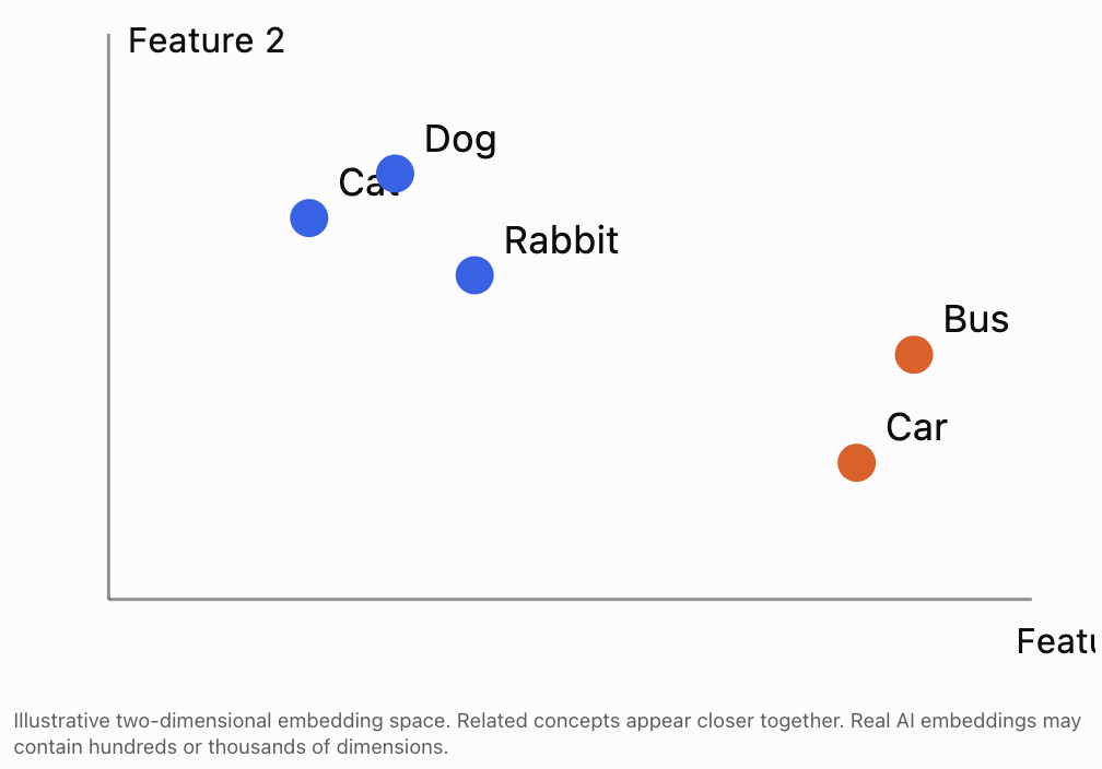
For example, a hypothetical AI system might represent three words using vectors:
These values are illustrative rather than actual embeddings from a trained model.
The vectors for cat and dog are close together, while car is farther away.
In a trained embedding system, such relationships may reflect similarities learned from data.
Why Embeddings Matter
Embeddings make it possible to compare information mathematically.
They are used in:
-
Search engines.
-
Language models.
-
Recommendation systems.
-
Image retrieval.
-
Document classification.
-
Semantic search.
However, the numerical meaning of each individual embedding coordinate is not always directly interpretable.
Matrices in Neural Networks
A neural network is a computational model containing layers of interconnected numerical operations.
Many neural networks use matrix multiplication to transform input data.
A basic layer can be written as:
where:
-
x is the input vector.
-
W is a weight matrix.
-
b is a bias vector.
-
z is the output before applying an activation function.
An activation function is often applied:
The activation function introduces nonlinearity, allowing neural networks to represent relationships more complex than a single linear transformation.
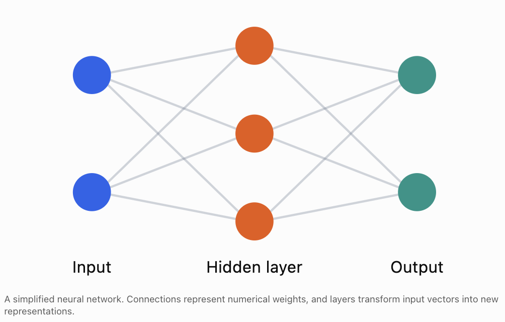
Worked Example 7: A Simple Neural Network Layer
Suppose:
Input:
Bias:
Calculate:
First multiply:
Add the bias:
If the layer uses the ReLU activation function:
then:
The output is the transformed feature vector.
How Neural Networks Learn
A neural network begins with numerical weights and biases.
During training, the network processes examples and compares its predictions with known targets.
A loss function measures prediction error.
The training process then adjusts the weights and biases to reduce the loss.
A common optimisation method is gradient descent.
For a parameter w:
where:
-
L is the loss function.
-
α is the learning rate.
-
dL/dw is the derivative of loss with respect to the weight.
For many parameters collected into a vector:
The gradient indicates how the loss changes as the parameters change.
Worked Example 8: One Gradient Descent Step
Suppose:
w = 5
Learning rate:
α = 0.1
Gradient:
dL/dw = 6
Calculate the updated weight.
The weight decreases from 5 to 4.4.
This is one small step in the training process.
Modern neural networks may contain millions or billions of parameters, and training involves many such updates.
Image Data as Matrices
Digital images are represented using numerical values.
A grayscale image can be stored as a matrix.
Each matrix entry represents the intensity of a pixel.
For a typical 8-bit grayscale image:
-
0 represents black.
-
255 represents white.
-
Values between 0 and 255 represent shades of gray.
Consider:
This represents a 3 × 3 grayscale image.
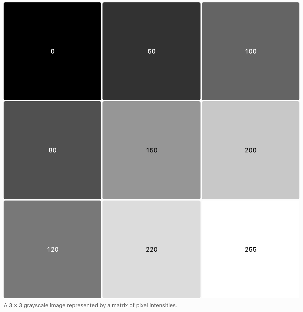
Image Brightness
To increase brightness, a positive value can be added to every pixel.
For example:
Adding 30 gives:
Pixel values must remain within the allowed range.
If a calculation produces a value greater than 255, it may be clipped to 255.
Colour Images
Colour images are commonly represented using three channels:
-
Red.
-
Green.
-
Blue.
Each channel is a matrix.
A colour image can therefore be represented as a three-dimensional array of numerical values.
This representation is used in computer vision and image-processing systems.
Data Transformations and Dimensionality Reduction
Real datasets may contain hundreds or thousands of features.
Some features may be redundant or strongly related.
Dimensionality reduction attempts to represent data using fewer variables while retaining useful information.
One important method is Principal Component Analysis (PCA).
PCA identifies directions in the data along which variation is greatest.
These directions are called principal components.
They are calculated using eigenvectors of a covariance matrix or equivalent numerical methods.
Worked Example 9: A Simple Data Projection
Suppose:
We want to project this vector onto the x-axis.
The projection matrix is:
Calculate:
Therefore:
The original two-dimensional vector has been projected onto a one-dimensional subspace.
This illustrates the basic idea of representing data using fewer dimensions.
PCA chooses projection directions based on the structure of the dataset rather than simply choosing the x-axis.
Recommendation Systems
Recommendation systems suggest products, films, music, or other content based on available information.
One approach represents users and items as vectors in a shared feature space.
For example, a user preference vector might be:
The components might represent preferences for:
-
Action.
-
Comedy.
-
Science fiction.
A film might have feature vector:
A simple compatibility score can be calculated using the dot product.
Worked Example 10: Recommendation Score
A larger dot product may indicate greater compatibility in this simplified model.
However, dot products also depend on vector magnitudes, so real recommendation systems often use normalisation or more sophisticated methods.
Matrices and Modern Computing
Matrix calculations appear throughout modern computing.
Graphics Processing Units
A GPU is a processor designed to perform many calculations in parallel.
GPUs are especially effective for operations involving large arrays and matrices.
This makes them valuable for:
-
Computer graphics.
-
Scientific simulations.
-
Image processing.
-
Neural network training.
-
Large-scale numerical computing.
Why Matrix Operations Are Efficient
Suppose a neural network needs to process 10,000 observations.
Instead of calculating each prediction separately, the observations can be arranged into a matrix.
The computer can then perform matrix operations on many observations together.
Specialised hardware and numerical libraries can carry out these operations efficiently.
Matrices in Language Models
Language models process text by converting tokens into numerical vector representations.
These vectors are transformed through multiple computational layers.
Matrix multiplication is used extensively in these transformations.
One important mechanism is attention, which helps a model combine information from different positions in a sequence.
A simplified attention calculation is:
where:
-
Q contains query vectors.
-
K contains key vectors.
-
V contains value vectors.
-
dₖ is the dimension of each key vector.
-
softmax converts numerical scores into relative weights.
This is an advanced example of how linear algebra supports modern AI.
The essential idea is that matrices allow a model to compare and combine many vector representations efficiently.
Real-World Applications
Medical Imaging
AI systems analyse numerical representations of medical images to help identify patterns that may be relevant to diagnosis. Matrix operations are central to image processing and neural networks.
Recommendation Systems
Streaming and shopping platforms use numerical representations of users and items to estimate preferences and recommend content.
Autonomous Vehicles
Cameras and sensors generate numerical data. AI systems use vectors, matrices, and transformations to analyse surroundings and support navigation decisions.
Scientific Research
Researchers use matrix methods to organise large datasets, fit models, reduce dimensionality, and investigate relationships among variables.
Robotics
Robots use matrices to transform coordinates, process sensor data, recognise objects, and calculate movement.
Limitations and Responsible Use of AI
Although vectors and matrices provide powerful tools for analysing data, mathematical models are not automatically accurate or fair.
Several important limitations must be considered.
Data Quality
A model trained using incomplete or inaccurate data may produce unreliable predictions.
Bias
If training data reflects unfair patterns or underrepresents certain groups, a model may reproduce or amplify those patterns.
Overfitting
A model may perform extremely well on training data but poorly on new observations.
This is called overfitting.
Interpretability
Some models are difficult to interpret because their predictions depend on many interacting numerical parameters.
Correlation and Causation
A model may identify statistical relationships without establishing causal explanations.
Privacy
Datasets may contain sensitive information. Responsible systems require appropriate privacy and security safeguards.
Model Evaluation
AI systems should be tested using suitable data and performance measures.
A model's usefulness depends not only on mathematical calculations but also on the quality of its assumptions, data, evaluation, and application.
Common Mistakes
Mistake 1: Assuming every vector represents a physical direction
In data science, vector components often represent features rather than spatial coordinates.
Mistake 2: Mixing up rows and columns in a data matrix
Rows commonly represent observations, while columns represent features, although other conventions are possible.
Mistake 3: Multiplying matrices with incompatible dimensions
The number of columns in the first matrix must equal the number of rows in the second.
Mistake 4: Assuming matrix multiplication is commutative
In general:
AB ≠ BA
Mistake 5: Ignoring feature scales
Features with large numerical values may dominate some calculations unless appropriate scaling is used.
Mistake 6: Confusing Euclidean distance with cosine similarity
Euclidean distance measures separation. Cosine similarity measures directional alignment.
Mistake 7: Assuming a larger dot product always means greater similarity
Dot products depend on both magnitude and direction.
Mistake 8: Thinking neural networks use only linear operations
Nonlinear activation functions are essential for representing many complex relationships.
Mistake 9: Assuming AI models automatically understand the meaning of numbers
The meaning of numerical features depends on how the data is represented and how the model is trained.
Mistake 10: Confusing training accuracy with generalisation
A model may fit training data well but perform poorly on unseen examples.
Mistake 11: Assuming PCA always preserves all information
Dimensionality reduction may discard some information.
Mistake 12: Assuming mathematical predictions are always correct
Predictions depend on the model, its assumptions, and the quality of the data.
Key Terms
-
Data Science: Study of collecting, organising, analysing, and interpreting data.
-
Artificial Intelligence: Field concerned with computational systems performing tasks associated with intelligent behaviour.
-
Machine Learning: Approach in which computational models learn patterns from data.
-
Feature: Measurable characteristic used to describe an observation.
-
Feature Vector: Ordered collection of numerical features.
-
Data Matrix: Matrix containing observations and features.
-
Weight: Numerical parameter describing the contribution of a feature or connection.
-
Bias: Additive parameter in a mathematical model.
-
Prediction: Output estimated by a model.
-
Linear Regression: Method for modelling numerical relationships using linear equations.
-
Residual: Difference between an observed value and a predicted value.
-
Loss Function: Function measuring model error.
-
Least Squares: Method that minimises the sum of squared residuals.
-
Feature Scaling: Transformation of numerical features to more suitable scales.
-
Min-Max Scaling: Method transforming values using their minimum and maximum.
-
Standardisation: Transformation expressing values relative to a mean and standard deviation.
-
Euclidean Distance: Straight-line distance between vectors.
-
Dot Product: Scalar obtained by multiplying and summing corresponding vector components.
-
Cosine Similarity: Measure of directional similarity between nonzero vectors.
-
Vector Space: Mathematical structure supporting vector addition and scalar multiplication.
-
Embedding: Numerical vector representation of an object or concept.
-
Neural Network: Computational model consisting of interconnected layers of numerical operations.
-
Activation Function: Function applied to a neuron's or layer's numerical output.
-
ReLU: Activation function defined by f(x) = max(0, x).
-
Gradient Descent: Optimisation method that updates parameters using gradients.
-
Learning Rate: Parameter controlling the size of optimisation updates.
-
Pixel: Smallest individual element of a raster image.
-
Principal Component Analysis: Technique for finding directions of greatest variation in data.
-
Dimensionality Reduction: Process of representing data using fewer features.
-
Recommendation System: System that predicts or suggests items based on available information.
-
GPU: Graphics processing unit designed for highly parallel computation.
-
Overfitting: When a model learns training-specific patterns that do not generalise well.
-
Generalisation: Ability of a model to perform effectively on new data.
-
Attention: Mechanism that combines information using learned relevance weights.
Key Takeaways
-
Vectors provide numerical representations of observations and features.
-
Data matrices organise multiple observations into rows and features into columns.
-
Matrix operations allow computers to process large datasets efficiently.
-
Weighted predictions can be calculated using dot products.
-
Linear regression uses vectors and matrices to model numerical relationships.
-
Feature scaling helps make numerical variables more comparable.
-
Euclidean distance measures separation between data vectors.
-
Cosine similarity measures directional alignment between vectors.
-
AI embeddings represent objects and concepts as vectors in high-dimensional spaces.
-
Neural networks use matrix multiplication, biases, and activation functions to transform data.
-
Gradient descent adjusts model parameters to reduce prediction error.
-
Digital images can be represented using matrices of pixel intensities.
-
PCA uses linear algebra to reduce the number of dimensions needed to represent data.
-
Recommendation systems can compare user and item vectors.
-
GPUs accelerate many large-scale matrix operations.
-
Modern language models rely heavily on vector representations and matrix calculations.
-
Responsible AI requires attention to data quality, fairness, privacy, and model evaluation.
Check Your Understanding
Questions
Question 1: Feature Vectors
A student has the following characteristics:
-
Study hours: 6
-
Assignments completed: 9
-
Test score: 78
Represent the student as a feature vector.
Question 2: Data Matrices
Three students have the following data:
|
Student |
Study hours |
Test score |
|---|---|---|
|
A |
4 |
60 |
|
B |
6 |
75 |
|
C |
8 |
90 |
Construct a data matrix.
Question 3: Matrix Dimensions
A dataset contains 200 observations and 5 numerical features.
What are the dimensions of its data matrix if observations are rows?
Question 4: Matrix Multiplication
Calculate:
Question 5: Weighted Prediction
A prediction model is:
Calculate the prediction when:
x₁ = 5
x₂ = 8
Question 6: Multiple Predictions
Given:
and:
Calculate Xw.
Question 7: Prediction Error
Actual values are:
10, 15, 20
Predicted values are:
12, 14, 18
Calculate the sum of squared errors.
Question 8: Feature Scaling
A dataset has a minimum value of 20 and maximum value of 80.
Calculate the min-max scaled value of 50.
Question 9: Euclidean Distance
Calculate the distance between:
and:
Question 10: Cosine Similarity
Calculate the cosine similarity between:
and:
Question 11: Neural Network Layer
Given:
and:
Calculate Wx + b.
Question 12: Gradient Descent
A weight has initial value 8.
The gradient is 5 and the learning rate is 0.2.
Calculate the updated weight.
Question 13: Image Processing
A grayscale image has pixel matrix:
Increase every pixel value by 20, clipping values at 255 if necessary.
Question 14: Data Science Concepts
Explain the difference between:
a) A feature vector and a data matrix.
b) Euclidean distance and cosine similarity.
c) Training performance and generalisation.
Question 15: Integrated AI Modelling Challenge
A simple AI system predicts the suitability of an educational resource using three features:
-
Content quality.
-
Difficulty match.
-
Student interest.
A resource has feature vector:
The model uses:
and bias:
b = 1
a) Calculate the weighted prediction.
b) Explain the meaning of the weights.
c) Calculate the new prediction if student interest increases from 9 to 10.
d) Explain why this model is linear.
e) Identify two limitations of using this model to recommend educational resources.
Fully Worked Answers
Answer 1: Feature Vectors
The three features are:
Study hours = 6
Assignments completed = 9
Test score = 78
Therefore:
The vector belongs to ℝ³.
Answer 2: Data Matrices
Each row represents one student.
The columns represent study hours and test score.
This is a 3 × 2 matrix.
Answer 3: Matrix Dimensions
There are:
200 observations.
5 features.
Therefore:
The matrix contains 200 rows and 5 columns.
Answer 4: Matrix Multiplication
First row:
2(5) + 3(2) = 16
Second row:
4(5) + 1(2) = 22
Therefore:
Answer 5: Weighted Prediction
Substitute:
Answer 6: Multiple Predictions
First row:
2(3) + 3(2) = 12
Second row:
4(3) + 5(2) = 22
Therefore:
Answer 7: Prediction Error
Residuals:
10 − 12 = −2
15 − 14 = 1
20 − 18 = 2
Square:
(−2)² = 4
1² = 1
2² = 4
Therefore:
Answer 8: Feature Scaling
Substitute:
Answer 9: Euclidean Distance
Answer 10: Cosine Similarity
Dot product:
Both vectors have magnitude 1.
Therefore:
The vectors are perpendicular.
Answer 11: Neural Network Layer
First calculate:
First component:
1(2) + 2(4) = 10
Second component:
3(2) + 1(4) = 10
Therefore:
Add the bias:
Answer 12: Gradient Descent
Substitute:
Answer 13: Image Processing
Original:
Add 20:
All values remain within the permitted range of 0 to 255.
Therefore:
Answer 14: Data Science Concepts
Part a: Feature vector versus data matrix
A feature vector represents the numerical characteristics of one observation.
A data matrix represents multiple observations, usually with each row corresponding to one observation and each column to one feature.
Part b: Euclidean distance versus cosine similarity
Euclidean distance measures the straight-line separation between two vectors.
Cosine similarity measures how closely their directions align.
Part c: Training performance versus generalisation
Training performance measures how well a model fits the examples used during training.
Generalisation describes how well the model performs on new, previously unseen observations.
A model may perform well during training but generalise poorly.
Answer 15: Integrated AI Modelling Challenge
Given:
and:
b = 1
Part a: Weighted prediction
Part b: Meaning of weights
The weights describe how strongly each feature contributes to the model's prediction when the other features remain fixed.
The model gives:
-
Content quality a weight of 0.4.
-
Difficulty match a weight of 0.3.
-
Student interest a weight of 0.2.
The relative importance of these weights depends on how the features are scaled.
Part c: Increased student interest
New feature vector:
Calculate:
The prediction increases by 0.2.
Part d: Why the model is linear
The model uses a weighted sum of the features, followed by addition of a constant bias.
More precisely, it is an affine model because of the nonzero bias. Its dependence on the input features is linear apart from that constant offset.
Part e: Limitations
Two limitations are:
-
The model assumes each feature contributes independently and at a constant rate. Real educational suitability may depend on interactions between features.
-
The model does not include other important factors such as learning style, prior knowledge, accessibility, or resource quality beyond the chosen numerical measures.
Therefore, the model provides a simplified estimate rather than a complete assessment of educational suitability.
Final Reflection
Vectors and matrices are essential mathematical tools in modern data science and artificial intelligence.
Vectors allow numerical information to be represented in a consistent mathematical form. Matrices organise large collections of observations and make it possible to process data efficiently.
Machine learning models use weighted combinations of features to generate predictions. Neural networks extend these ideas through repeated matrix operations and nonlinear transformations.
Vector spaces allow AI systems to represent complex information, including words, images, documents, and user preferences, using high-dimensional numerical representations.
Linear algebra also supports image processing, dimensionality reduction, recommendation systems, optimisation, and large-scale computing.
However, the mathematical power of AI must be combined with careful data collection, responsible model design, appropriate evaluation, and an understanding of limitations.
The central idea is that vectors and matrices transform information into mathematical structures that computers can analyse, compare, and use to identify patterns and generate predictions.
4. Optimisation and Mathematical Modelling
Learning outcomes
- I can model optimisation problems using vectors and matrices.
- I can analyse systems with multiple variables.
- I can evaluate mathematical models.
- I can justify modelling choices.
- I can solve authentic optimisation problems.
Introduction
Many important problems in mathematics, science, engineering, economics, and technology involve finding the best possible solution.
A company may want to maximise profit while limiting production costs. An engineer may need to minimise the weight of a structure while maintaining its strength. A transport company may want to reduce travel distances while meeting delivery requirements. A scientist may need to determine the combination of variables that produces the most accurate mathematical model.
These are examples of optimisation problems.
Optimisation involves finding the maximum or minimum value of a quantity while satisfying any necessary conditions or restrictions.
Vectors and matrices are particularly useful because they allow us to represent many variables and constraints in a compact, organised mathematical form.
In this lesson, we will investigate how to construct optimisation models, analyse systems involving multiple variables, solve linear and quadratic optimisation problems, evaluate mathematical assumptions, and apply optimisation to authentic situations.
What Is Optimisation?
Optimisation is the process of finding the best possible value of an objective, subject to any relevant constraints.
The objective may be to:
-
Maximise profit, output, efficiency, or performance.
-
Minimise cost, energy consumption, travel distance, error, or waste.
-
Find the best combination of resources.
-
Determine the most accurate parameters for a mathematical model.
An optimisation problem usually contains three important components.
Decision variables are quantities we can choose or control.
Objective function is the mathematical expression we want to maximise or minimise.
Constraints are restrictions that the solution must satisfy.
For example, suppose a company produces two products.
Let:
x = number of units of Product A.
y = number of units of Product B.
If each unit of A earns $30 profit and each unit of B earns $20 profit, the objective function is:
The company wants to maximise P.
However, production may be limited by available labour, materials, or machine time.
These limitations become constraints.
Representing Optimisation Problems Using Vectors
When an optimisation problem contains several decision variables, we can organise them into a vector.
For three variables:
The objective can also be represented using a vector of coefficients:
For a linear objective function:
we can write:
Here, cᵀ is the transpose of the coefficient vector.
This is the dot product of the coefficient vector and the decision-variable vector.
Worked Example 1: A Profit Model
A manufacturer produces three products.
|
Product |
Profit per unit |
|---|---|
|
A |
$12 |
|
B |
$18 |
|
C |
$25 |
The company produces:
-
40 units of A.
-
30 units of B.
-
20 units of C.
Represent the production and profit information using vectors, then calculate total profit.
The production vector is:
The profit coefficient vector is:
Total profit:
This example demonstrates how a dot product can calculate an objective function involving several variables.
Representing Constraints Using Matrices
Suppose a factory produces three products using two limited resources.
Each product requires different quantities of labour and material.
|
Resource |
Product A |
Product B |
Product C |
Available |
|---|---|---|---|---|
|
Labour hours |
2 |
3 |
4 |
120 |
|
Material units |
5 |
2 |
3 |
150 |
Let:
x₁ = number of units of A.
x₂ = number of units of B.
x₃ = number of units of C.
The labour constraint is:
The material constraint is:
These can be written as:
where:
The inequality is interpreted component by component.
We also require:
because production quantities cannot be negative.
General Linear Optimisation Model
A common form of a linear programming problem is:
subject to:
and:
This mathematical structure is widely used in operations research, manufacturing, transportation, logistics, and resource allocation.
Feasible Regions
The feasible region is the set of all solutions that satisfy every constraint.
In a two-variable problem, the feasible region can be represented graphically.
For example, consider:
The first inequality describes points on or below the line:
x + y = 8
The second inequality describes points on or below:
2x + y = 12
The non-negativity constraints restrict the solution to the first quadrant.
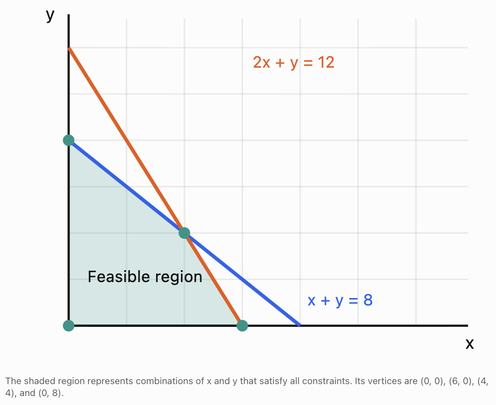
Every point inside or on the boundary of the feasible region is an allowable solution.
Points outside the region violate at least one constraint.
Linear Programming
Linear programming is the process of optimising a linear objective function subject to linear constraints.
When there are two decision variables, many problems can be solved graphically.
An important result is that if a linear objective has a maximum or minimum over a nonempty, bounded polygonal feasible region, at least one optimal solution occurs at a vertex.
This is called the corner-point principle.
Worked Example 2: Maximising Factory Profit
A factory manufactures two products.
Product A earns $40 profit per unit.
Product B earns $30 profit per unit.
The constraints are:
Find the maximum possible profit.
Step 1: Write the objective function
Step 2: Find the vertices of the feasible region
The vertices include:
(0, 0)
(50, 0)
(0, 40)
We must also find the intersection of:
2x + y = 100
x + 2y = 80
From the first equation:
y = 100 − 2x
Substitute into the second:
x + 2(100 − 2x) = 80
x + 200 − 4x = 80
−3x = −120
Then:
The intersection is:
(40, 20)
Step 3: Evaluate the objective at each vertex
|
Vertex |
Profit calculation |
Profit |
|---|---|---|
|
(0, 0) |
40(0) + 30(0) |
$0 |
|
(50, 0) |
40(50) + 30(0) |
$2,000 |
|
(0, 40) |
40(0) + 30(40) |
$1,200 |
|
(40, 20) |
40(40) + 30(20) |
$2,200 |
Step 4: Identify the maximum
The greatest profit is $2,200.
Therefore:
The factory should produce 40 units of A and 20 units of B.
Step 5: Interpret the result
Both resource constraints are fully used:
This means the optimal solution uses all available quantities of both constrained resources.
Integer Programming
Some optimisation variables must be whole numbers.
For example:
-
Number of vehicles.
-
Number of employees.
-
Number of machines.
-
Number of products.
-
Number of classrooms.
A solution such as 3.7 vehicles is not meaningful.
An integer programming problem includes restrictions requiring selected variables to be integers.
Worked Example 3: Whole-Number Production
A workshop produces chairs and tables.
Let:
x = number of chairs.
y = number of tables.
The profit is:
The constraints are:
and x and y must be integers.
The intersection of the two boundary lines is:
x + 2y = 9
2x + y = 10
Multiply the first equation by 2:
2x + 4y = 18
Subtract the second:
3y = 8
Then:
The continuous intersection is:
But fractional chairs and tables are not allowed.
We must examine feasible integer combinations.
|
Chairs |
Tables |
Profit |
|---|---|---|
|
3 |
3 |
$195 |
|
4 |
2 |
$180 |
|
2 |
3 |
$170 |
|
1 |
4 |
$185 |
|
5 |
0 |
$125 |
|
0 |
4 |
$160 |
The highest profit among these feasible combinations is $195. To verify global optimality, note that for each integer y = 0, 1, 2, 3, 4, the maximum feasible x is respectively 5, 4, 4, 3, 1. Their best profits are $125, $140, $180, $195, and $185.
Therefore:
This illustrates why integer constraints can change an optimisation problem.
Optimisation with Several Variables
Many real problems involve more than two variables.
Suppose a delivery company uses three types of vehicles.
Let:
x₁ = number of small vehicles.
x₂ = number of medium vehicles.
x₃ = number of large vehicles.
Suppose operating costs are:
$80, $120, and $180 per vehicle.
The cost function is:
In vector form:
where:
The company may need to satisfy capacity requirements:
and a vehicle availability constraint:
The objective is to minimise cost.
This model is an integer linear programming problem if all vehicle counts must be whole numbers.
In higher-dimensional problems, graphical methods become impractical.
Algorithms such as the simplex method, interior-point methods, and branch-and-bound are used to solve appropriate optimisation problems.
Quadratic Optimisation
Not all optimisation problems have linear objective functions.
A quadratic objective function contains squared variables or products of variables.
For example:
This function measures the squared distance of a point (x, y) from the origin.
To minimise it without additional constraints:
Therefore:
Matrix Form of a Quadratic Function
A quadratic function can be written using matrices:
where Q is a square matrix.
For example:
and:
Then:
Quadratic optimisation is used in:
-
Engineering design.
-
Portfolio optimisation.
-
Control systems.
-
Statistical modelling.
-
Machine learning.
Optimisation Using Calculus
Calculus provides methods for finding maximum and minimum values of differentiable functions.
For a function of one variable:
stationary points occur where:
These points may be maxima, minima, or neither.
Worked Example 4: Minimising a Cost Function
Suppose the cost of operating a machine is modelled by:
where x represents an adjustable operating setting.
Find the value of x that minimises cost.
Step 1: Differentiate
Step 2: Set the derivative equal to zero
Step 3: Confirm a minimum
Since:
the function has a minimum at x = 10.
Step 4: Calculate the minimum cost
The minimum cost is 100 cost units at operating setting x = 10.
Optimisation with Multiple Variables
For a function involving several variables:
we use partial derivatives.
The gradient is:
At an interior stationary point of a differentiable function:
Worked Example 5: Minimising a Two-Variable Function
Find the minimum of:
Step 1: Calculate partial derivatives
Step 2: Set both equal to zero
Step 3: Evaluate the function
Step 4: Confirm the minimum
Complete the square:
Since squared terms cannot be negative:
at:
This is the global minimum.
The Hessian Matrix
For functions involving multiple variables, second derivatives can be organised into a matrix called the Hessian.
For f(x, y):
For:
the Hessian is:
This matrix is positive definite.
Therefore, the stationary point is a strict local minimum.
Because the function is a convex quadratic, it is also the global minimum.
Interpreting the Hessian
At a stationary point:
-
A positive definite Hessian indicates a strict local minimum.
-
A negative definite Hessian indicates a strict local maximum.
-
An indefinite Hessian indicates a saddle point.
-
A semidefinite Hessian may require further analysis.
The Hessian connects multivariable calculus directly to matrix algebra.
Least-Squares Optimisation
A major application of optimisation is finding a mathematical model that fits observed data.
Suppose a linear model is:
We want to choose m and b so that predictions are close to the actual observations.
The least-squares objective is:
The goal is to minimise SSE.
Matrix Representation
A linear model can be written as:
where:
-
A is the design matrix.
-
β is the vector of model parameters.
-
y is the vector of observed values.
The least-squares problem is:
When A has linearly independent columns, the unique least-squares solution satisfies:
These are called the normal equations.
If AᵀA is invertible:
In practical numerical computing, QR factorisation or singular value decomposition is often preferred to explicitly forming this inverse.
Worked Example 6: Fitting a Line
Suppose the observations are:
|
x |
y |
|---|---|
|
1 |
2 |
|
2 |
3 |
|
3 |
5 |
Find the least-squares regression line.
We use:
The means are:
The slope is:
Numerator:
Denominator:
Therefore:
The intercept is:
The regression equation is:
This line minimises the sum of squared vertical residuals for the observations.
Gradient Descent
Some optimisation problems are too large or complicated to solve directly.
Gradient descent is an iterative method that adjusts variables in the direction opposite to the gradient.
The update rule is:
where:
-
xₖ is the current estimate.
-
α is the learning rate or step size.
-
∇f is the gradient.
The gradient points in the direction of steepest local increase, so moving against it can reduce the objective function.
Worked Example 7: Gradient Descent
Consider:
The derivative is:
Start with:
x₀ = 5
Use learning rate:
α = 0.1
The update rule is:
First iteration:
Second iteration:
Third iteration:
The values move toward zero, where f(x) reaches its minimum.
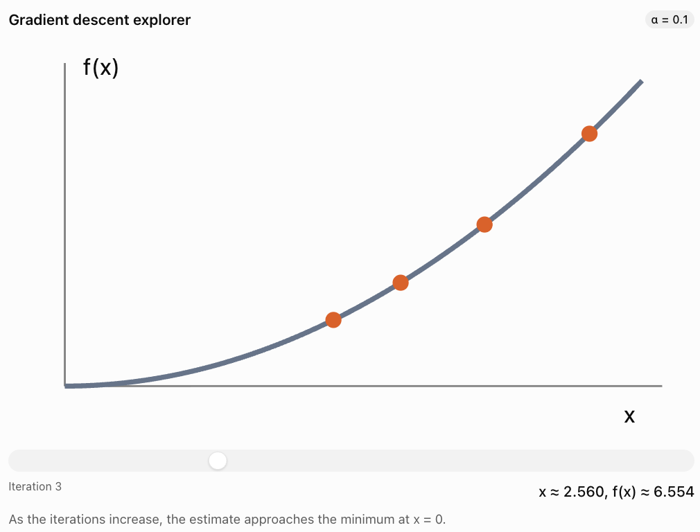
Choosing a Learning Rate
If the learning rate is too small, convergence may be slow.
If it is too large, the algorithm may overshoot the minimum or fail to converge.
Gradient descent is widely used in machine learning, optimisation, and scientific computing.
Constrained Optimisation Using Lagrange Multipliers
Some optimisation problems involve equality constraints.
For example, we may want to maximise a function:
subject to:
The method of Lagrange multipliers introduces a new variable λ.
At a suitable constrained optimum:
together with:
Worked Example 8: Maximum Product with Fixed Sum
Find the maximum value of:
subject to:
with x, y ≥ 0.
The gradients are:
Set:
Therefore:
y = λ
x = λ
Hence:
x = y
Using the constraint:
x + y = 10
2x = 10
x = 5
y = 5
Therefore:
We can verify this result using substitution:
This is a downward-opening parabola with maximum at x = 5.
The maximum product occurs when the two nonnegative numbers are equal.
Mathematical Modelling in Engineering
Engineering optimisation often involves balancing competing requirements.
For example, a structural engineer may want to minimise the mass of a component while ensuring that it can support a specified load.
A general engineering optimisation model might be:
subject to:
and:
where the decision vector x may contain dimensions, material quantities, or operating parameters.
The constraints may represent:
-
Maximum stress.
-
Minimum strength.
-
Maximum displacement.
-
Available materials.
-
Safety requirements.
-
Manufacturing limitations.
Example: Minimising Material Cost
Suppose a rectangular container has a fixed volume:
The surface area of a closed rectangular container is:
If material cost is proportional to surface area, minimising material cost means minimising S.
The constraint is:
This is a nonlinear constrained optimisation problem.
For a closed rectangular box with a fixed positive volume and no other restrictions, the minimum surface area occurs when:
The optimal shape is a cube.
This result illustrates how mathematical modelling can guide engineering design.
Optimisation in Transportation and Logistics
Transport companies frequently solve optimisation problems involving:
-
Vehicle capacity.
-
Delivery demand.
-
Fuel consumption.
-
Travel time.
-
Driver availability.
-
Storage limitations.
Worked Example 9: A Transportation Model
A supplier has two warehouses and two stores.
Warehouse A can supply 40 units.
Warehouse B can supply 60 units.
Store 1 requires 50 units.
Store 2 requires 50 units.
Shipping costs per unit are:
|
Route |
Store 1 |
Store 2 |
|---|---|---|
|
Warehouse A |
$4 |
$6 |
|
Warehouse B |
$5 |
$3 |
Let:
x₁₁ = units shipped from A to Store 1.
x₁₂ = units shipped from A to Store 2.
x₂₁ = units shipped from B to Store 1.
x₂₂ = units shipped from B to Store 2.
The objective is:
Constraints:
Warehouse A:
Warehouse B:
Store 1:
Store 2:
All variables must be nonnegative.
Step 1: Express all variables using one variable
Let:
Then:
Non-negativity requires:
Step 2: Substitute into the cost function
Expand:
Simplify:
Step 3: Minimise cost
Since the coefficient of t is negative, cost decreases as t increases.
Therefore, choose the largest feasible value:
Step 4: Calculate shipment quantities
Step 5: Calculate minimum cost
The optimal shipping plan is:
-
40 units from Warehouse A to Store 1.
-
10 units from Warehouse B to Store 1.
-
50 units from Warehouse B to Store 2.
Multi-Objective Optimisation
Some problems have more than one objective.
For example, a company may want to:
-
Minimise cost.
-
Maximise quality.
-
Minimise environmental impact.
-
Maximise customer satisfaction.
These objectives may conflict.
A cheaper solution may produce lower quality.
A more environmentally sustainable solution may have higher initial costs.
Weighted Objective Functions
One approach combines objectives using weights.
Suppose:
C = cost.
E = environmental impact.
We may minimise:
where α and β represent the relative importance of each objective.
The quantities should be scaled appropriately before combining them, especially when measured in different units.
Pareto Optimality
A solution is Pareto optimal if no objective can be improved without making at least one other objective worse.
Rather than producing a single best solution, multi-objective optimisation may produce a collection of reasonable trade-offs.
This collection is called the Pareto frontier.
Evaluating Mathematical Models
A mathematically correct solution is not necessarily a useful real-world solution.
A model must also be evaluated in terms of its assumptions, limitations, and practical meaning.
Important Questions
1. Are the assumptions reasonable?
For example, does the model assume constant costs when costs actually change with production volume?
2. Are the variables clearly defined?
Every variable should have a precise interpretation and appropriate units.
3. Are all important constraints included?
A production model may be unrealistic if it ignores storage, labour availability, or maintenance.
4. Is the objective appropriate?
Maximising short-term profit may not be the same as maximising long-term sustainability.
5. Are the data reliable?
Incorrect estimates of cost, demand, or capacity may lead to poor decisions.
6. Is the solution practical?
A mathematically optimal solution may require fractional machines, impossible schedules, or unavailable resources.
7. How sensitive is the solution?
Would a small change in input data produce a very different answer?
Sensitivity Analysis
Sensitivity analysis examines how changes in model parameters affect the optimal solution.
Suppose a company maximises:
If the profit per unit of Product B increases from $30 to $50, the objective becomes:
The best production combination may change.
Worked Example 10: Sensitivity of an Optimal Solution
Return to the feasible vertices from Worked Example 2:
(0, 0), (50, 0), (0, 40), and (40, 20).
The new profit function is:
Evaluate:
|
Vertex |
New profit |
|---|---|
|
(0, 0) |
$0 |
|
(50, 0) |
$2,000 |
|
(0, 40) |
$2,000 |
|
(40, 20) |
$2,600 |
Therefore:
The optimal production quantities remain:
Although the profit increased, the optimal production combination did not change.
This demonstrates that some optimisation solutions are stable under certain changes in model parameters.
Choosing an Appropriate Optimisation Method
Different problems require different mathematical techniques.
|
Problem type |
Common method |
|---|---|
|
Linear objective, linear constraints |
Linear programming |
|
Whole-number decision variables |
Integer programming |
|
Smooth one-variable function |
Differentiation |
|
Smooth multivariable function |
Partial derivatives and gradients |
|
Quadratic objective with suitable constraints |
Quadratic programming |
|
Equality-constrained differentiable problem |
Lagrange multipliers |
|
Fitting a linear model to data |
Least squares |
|
Large differentiable optimisation problem |
Gradient-based methods |
|
Several competing objectives |
Multi-objective optimisation |
|
Complex discrete routing or scheduling |
Integer optimisation or specialised algorithms |
The best method depends on the mathematical structure of the problem.
Real-World Applications
Manufacturing and Production
Optimisation helps determine production quantities, resource allocation, staffing, and operating schedules to reduce costs or maximise output.
Transportation and Logistics
Mathematical models determine efficient shipping plans, delivery schedules, and vehicle assignments while satisfying demand and capacity constraints.
Engineering Design
Engineers optimise structures and systems to reduce weight, cost, and energy consumption while maintaining strength, safety, and performance.
Artificial Intelligence
Machine learning algorithms optimise model parameters to reduce prediction errors and improve performance on relevant tasks.
Energy Systems
Optimisation helps balance energy production, storage, demand, and operating costs in electrical networks and renewable energy systems.
Common Mistakes
Mistake 1: Confusing decision variables with fixed parameters
Decision variables are quantities we choose. Parameters are values supplied by the model.
Mistake 2: Writing an objective function without defining the variables
Every variable must have a clear interpretation.
Mistake 3: Forgetting constraints
An unconstrained maximum may be unrealistic or unbounded.
Mistake 4: Using the wrong inequality direction
For example, a maximum resource limit requires ≤, while a minimum demand requirement often requires ≥.
Mistake 5: Forgetting non-negativity restrictions
Negative production quantities or vehicle counts are usually not meaningful.
Mistake 6: Assuming every feasible solution is optimal
A feasible solution satisfies the constraints, but it may not maximise or minimise the objective.
Mistake 7: Assuming the optimum always occurs at a corner
The corner-point principle applies to linear objectives over appropriate polyhedral feasible regions. Nonlinear objectives may have interior optima.
Mistake 8: Ignoring integer restrictions
A fractional solution may not be practical when variables represent indivisible objects.
Mistake 9: Confusing local and global optima
A local optimum is best within a nearby region. A global optimum is best over the entire feasible set.
Mistake 10: Assuming every stationary point is a minimum
Stationary points may be minima, maxima, or saddle points.
Mistake 11: Applying matrix formulas without checking dimensions
Matrix multiplication requires compatible dimensions.
Mistake 12: Assuming the inverse of AᵀA always exists
The inverse requires the columns of A to be linearly independent.
Mistake 13: Choosing a learning rate without considering convergence
An inappropriate step size can slow or destabilise gradient descent.
Mistake 14: Ignoring model assumptions
A mathematically valid answer may not represent real conditions accurately.
Mistake 15: Treating an optimal solution as permanently optimal
Changes in prices, demand, resource availability, or constraints may change the best solution.
Key Terms
-
Optimisation: Process of finding the best value of an objective under specified conditions.
-
Mathematical Model: Mathematical representation of a real-world system.
-
Decision Variable: Quantity selected or controlled in an optimisation problem.
-
Parameter: Fixed numerical value used in a model.
-
Objective Function: Function to be maximised or minimised.
-
Constraint: Restriction on allowable solutions.
-
Feasible Solution: Solution satisfying every constraint.
-
Feasible Region: Set of all feasible solutions.
-
Optimal Solution: Feasible solution producing the best objective value.
-
Linear Programming: Optimisation involving linear objectives and constraints.
-
Integer Programming: Optimisation requiring some or all decision variables to be integers.
-
Corner-Point Principle: Property that a bounded linear programming problem with an optimum has an optimal vertex solution.
-
Dot Product: Scalar obtained by multiplying and summing corresponding vector components.
-
Constraint Matrix: Matrix containing coefficients of linear constraints.
-
Quadratic Optimisation: Optimisation involving quadratic objective functions.
-
Gradient: Vector of first-order partial derivatives.
-
Stationary Point: Point where the gradient is zero, when the gradient exists.
-
Hessian Matrix: Matrix of second-order partial derivatives.
-
Positive Definite Matrix: Symmetric matrix for which xᵀAx is positive for every nonzero vector x.
-
Convex Function: Function whose graph lies below or on the line segment connecting any two points on its graph.
-
Local Minimum: Minimum within a neighbourhood of a point.
-
Global Minimum: Smallest function value over the entire feasible domain.
-
Least Squares: Method minimising the sum of squared residuals.
-
Residual: Difference between an observed value and a predicted value.
-
Design Matrix: Matrix representing predictor variables in a statistical model.
-
Gradient Descent: Iterative optimisation method using the negative gradient.
-
Learning Rate: Step size used in gradient-based optimisation.
-
Lagrange Multiplier: Auxiliary variable used to analyse constrained optima.
-
Sensitivity Analysis: Study of how changes in parameters affect model results.
-
Multi-Objective Optimisation: Optimisation involving several objectives.
-
Pareto Optimality: Condition where improving one objective necessarily worsens another.
-
Pareto Frontier: Set of non-dominated trade-off solutions.
-
Model Validation: Process of checking whether a model adequately represents the intended system.
Key Takeaways
-
Optimisation involves maximising or minimising an objective while satisfying constraints.
-
Decision variables can be organised into vectors.
-
Linear objective functions can be expressed using dot products.
-
Systems of linear constraints can be represented using matrices.
-
The feasible region contains every solution satisfying all constraints.
-
Linear programming optimises linear objectives subject to linear constraints.
-
For suitable two-variable linear programming problems, optimal solutions can be found by evaluating vertices.
-
Integer programming is necessary when some variables must represent whole-number quantities.
-
Quadratic optimisation involves squared variables and can be represented using matrix expressions.
-
Differentiation and partial derivatives help identify stationary points.
-
The Hessian matrix helps classify stationary points of multivariable functions.
-
Least-squares optimisation is used to fit mathematical models to observed data.
-
Gradient descent provides an iterative method for minimising differentiable objective functions.
-
Lagrange multipliers help solve equality-constrained optimisation problems.
-
Transportation and production problems can be modelled using matrices and linear constraints.
-
Multi-objective optimisation considers trade-offs between competing goals.
-
Sensitivity analysis reveals how model results respond to changing assumptions.
-
A mathematically optimal solution must still be evaluated for realism, feasibility, and usefulness.
Check Your Understanding
Questions
Question 1: Objective Functions
A company produces two products.
Product A earns $15 profit per unit.
Product B earns $25 profit per unit.
Write an objective function for total profit.
Question 2: Vector Representation
A manufacturer produces three products with profits of $10, $20, and $30 per unit.
Write the profit coefficient vector.
Question 3: Dot Product
Given:
and:
Calculate cᵀx.
Question 4: Matrix Constraints
Write the following system in matrix form:
Question 5: Feasibility
Determine whether the point (5, 10) satisfies:
Question 6: Linear Programming
Maximise:
subject to:
Find the maximum value of P.
Question 7: Integer Programming
Explain why a company purchasing delivery trucks may require an integer programming model.
Question 8: Quadratic Optimisation
Find the minimum value of:
Question 9: Multivariable Optimisation
Find the minimum of:
Question 10: Gradient Descent
For:
start at x = 4 with learning rate α = 0.25.
Calculate the next two iterations.
Question 11: Least Squares
Actual values are:
10, 15, 20
Predicted values are:
12, 14, 19
Calculate the sum of squared errors.
Question 12: Transportation Costs
A company ships:
-
20 units at $4 per unit.
-
30 units at $6 per unit.
-
10 units at $8 per unit.
Calculate total shipping cost using a dot product.
Question 13: Sensitivity Analysis
A product earns $20 profit per unit.
The company produces 50 units.
Calculate total profit.
Then calculate the new profit if profit per unit increases to $24.
Question 14: Model Evaluation
Explain three reasons why a mathematically optimal solution might not be suitable in practice.
Question 15: Integrated Optimisation Challenge
A company produces two products, A and B.
Profit per unit:
A: $50
B: $40
Production constraints:
a) Define the decision variables.
b) Write the objective function.
c) Express the constraints in matrix form.
d) Find the vertices of the feasible region.
e) Calculate profit at each vertex.
f) Determine the optimal production quantities.
g) Calculate maximum profit.
h) Explain two assumptions of the model.
i) Explain how the model could be improved.
Fully Worked Answers
Answer 1: Objective Functions
Let:
x = number of units of A.
y = number of units of B.
Profit from A:
15x
Profit from B:
25y
Therefore:
The objective is to maximise P.
Answer 2: Vector Representation
The profit coefficient vector is:
Answer 3: Dot Product
Answer 4: Matrix Constraints
The system is:
Therefore:
Answer 5: Feasibility
Substitute:
x = 5
y = 10
First constraint:
Since:
20 ≤ 25
the first constraint is satisfied.
Second constraint:
Since:
35 ≤ 40
the second constraint is satisfied.
Therefore:
Answer 6: Linear Programming
Objective:
Constraints:
The vertices are:
(0, 0)
(6, 0)
(6, 4)
(2, 8)
(0, 8)
Evaluate:
|
Vertex |
P |
|---|---|
|
(0, 0) |
0 |
|
(6, 0) |
30 |
|
(6, 4) |
46 |
|
(2, 8) |
42 |
|
(0, 8) |
32 |
Therefore:
at:
Answer 7: Integer Programming
Delivery trucks cannot normally be purchased in fractional quantities.
A mathematical solution such as 4.6 trucks is not physically meaningful.
Therefore, the number of trucks must be restricted to nonnegative integers.
An integer programming model includes these restrictions.
Answer 8: Quadratic Optimisation
Given:
Differentiate:
Set equal to zero:
Evaluate:
Since the coefficient of x² is positive, the parabola opens upward and this is the global minimum.
Answer 9: Multivariable Optimisation
Given:
Partial derivatives:
Set equal to zero:
Evaluate:
Complete the square:
Therefore:
at:
Answer 10: Gradient Descent
Given:
Derivative:
Update rule:
Start:
x₀ = 4
First iteration:
Second iteration:
Therefore:
Answer 11: Least Squares
Residuals:
10 − 12 = −2
15 − 14 = 1
20 − 19 = 1
Square:
4, 1, 1
Add:
Answer 12: Transportation Costs
Cost vector:
Quantity vector:
Total cost:
Answer 13: Sensitivity Analysis
Original profit:
New profit:
Increase:
The total profit increases by $200, assuming the production quantity remains unchanged.
Answer 14: Model Evaluation
Three possible reasons are:
Unrealistic assumptions: The model may assume constant costs or unlimited demand when these conditions do not hold.
Missing constraints: The model may ignore labour availability, safety requirements, storage capacity, or environmental regulations.
Practical limitations: The solution may require fractional quantities, unavailable equipment, or unrealistic operating schedules.
A useful optimisation model must represent the important features of the real system.
Answer 15: Integrated Optimisation Challenge
Part a: Define variables
Let:
x = number of units of Product A.
y = number of units of Product B.
Part b: Objective function
The objective is to maximise P.
Part c: Matrix constraints
with:
Part d: Find the vertices
On the x-axis:
2x ≤ 100
Therefore:
x ≤ 50
Vertex:
(50, 0)
On the y-axis:
2y ≤ 80
Therefore:
y ≤ 40
Vertex:
(0, 40)
The origin is:
(0, 0)
Now solve:
2x + y = 100
x + 2y = 80
From the first equation:
y = 100 − 2x
Substitute:
x + 2(100 − 2x) = 80
x + 200 − 4x = 80
−3x = −120
Then:
Intersection:
(40, 20)
Therefore, the vertices are:
(0, 0), (50, 0), (0, 40), (40, 20).
Part e: Evaluate profit
|
Vertex |
Profit |
|---|---|
|
(0, 0) |
$0 |
|
(50, 0) |
$2,500 |
|
(0, 40) |
$1,600 |
|
(40, 20) |
$2,800 |
Part f: Optimal production
Part g: Maximum profit
Part h: Two assumptions
The model assumes that profit per unit remains constant regardless of production quantity.
It also assumes that the two resource constraints represent the important limitations on production.
Part i: Improvements
The model could be improved by including additional constraints such as labour availability, storage, customer demand, and machine maintenance.
It could also include changing production costs, uncertain demand, and sensitivity analysis.
These improvements would make the model more realistic and useful for decision-making.
Final Reflection
Optimisation and mathematical modelling connect abstract mathematical ideas with practical decision-making.
Vectors provide an organised way to represent decision variables. Matrices allow many constraints to be written and analysed efficiently. Linear programming identifies optimal solutions under linear restrictions, while calculus and quadratic optimisation extend these ideas to nonlinear relationships.
Least-squares methods and gradient descent demonstrate how optimisation is used to construct mathematical models from data. Engineering, transportation, economics, and artificial intelligence all rely on these techniques.
However, finding a mathematical optimum is only one part of solving a real-world problem. A successful model must also use realistic assumptions, appropriate constraints, reliable data, and meaningful interpretations.
The central idea is that optimisation uses mathematical models to identify the best available decisions while respecting the limitations and requirements of real systems.
5. Comprehensive Problem Solving
Learning outcomes
- I can solve complex multi-step problems involving vectors and matrices.
- I can integrate concepts from throughout the course.
- I can select efficient mathematical methods.
- I can justify mathematical reasoning.
- I can communicate complete mathematical solutions.
Introduction
Vectors and matrices are among the most powerful tools in mathematics because they allow us to represent, analyse, and solve problems involving several quantities simultaneously.
Throughout this course, we have explored how vectors describe magnitude and direction, how matrices represent transformations and systems of equations, and how linear algebra supports applications in science, engineering, computer graphics, data science, and artificial intelligence.
However, real-world mathematical problems rarely require just one isolated technique.
A navigation problem might combine vector addition, trigonometry, and simultaneous equations. An engineering problem might involve matrices, forces, and equilibrium conditions. A computer graphics problem may require several transformations applied in a particular order. A data science problem may combine matrix multiplication, regression, and optimisation.
Comprehensive problem solving involves recognising these connections and selecting the most appropriate mathematical tools.
In this lesson, we will integrate the major concepts from vectors and matrices, develop systematic problem-solving strategies, examine challenging multi-step applications, and practise communicating complete mathematical solutions.
The Mathematical Problem-Solving Process
Complex mathematical problems become more manageable when approached systematically.
A useful strategy involves six stages.
-
Understand the problem. Identify the known information, unknown quantities, units, and required result.
-
Construct a mathematical representation. Choose suitable vectors, matrices, equations, diagrams, or coordinate systems.
-
Select an efficient method. Decide whether vector operations, matrix algebra, determinants, inverses, elimination, or optimisation methods are appropriate.
-
Carry out the calculations. Work systematically, showing enough intermediate steps to make the solution clear.
-
Verify the solution. Substitute results into the original equations, check dimensions, and test whether physical constraints are satisfied.
-
Interpret and communicate. State what the mathematical result means in the original context, including units and limitations.
This process is particularly important when a problem requires several different mathematical ideas.
Reviewing the Main Tools of Linear Algebra
Before solving integrated problems, we should recognise the major mathematical techniques available.
|
Mathematical concept |
Main purpose |
Typical application |
|---|---|---|
|
Vector addition |
Combine quantities with direction |
Displacement and forces |
|
Scalar multiplication |
Change vector magnitude |
Velocity and scaling |
|
Dot product |
Calculate projections, work, or angles |
Physics and similarity |
|
Cross product |
Find perpendicular vectors and moments |
Mechanics and geometry |
|
Matrix multiplication |
Combine transformations or relationships |
Graphics and data analysis |
|
Determinants |
Test invertibility and measure area or volume scaling |
Geometry and systems |
|
Inverse matrices |
Reverse an invertible transformation |
Solving systems |
|
Gaussian elimination |
Solve simultaneous linear equations |
Engineering and modelling |
|
Eigenvalues and eigenvectors |
Identify invariant directions and scaling factors |
Dynamics and data science |
|
Matrix modelling |
Represent relationships between variables |
Economics and science |
|
Optimisation |
Find the best feasible solution |
Production and resource allocation |
The key skill is not simply remembering these techniques. It is recognising which technique is appropriate and why.
Choosing an Efficient Mathematical Method
Different mathematical problems suggest different approaches.
Interactive method selector
Choose the type of problem you need to solve.
Recommended approach: Gaussian elimination or matrix methods
Represent the equations as A x = b. Row reduction is generally reliable, including when a matrix is singular. For a small invertible system, an inverse may also be useful.
Verification: Substitute the solution into every original equation.
A good mathematician selects a method based on the structure of the problem rather than applying the same procedure to every situation.
Integrated Problem 1: Navigation Using Vectors
A rescue boat travels 12 km east and then 9 km north.
A current subsequently causes an additional displacement of 3 km west and 4 km south.
Determine the boat's final displacement from its starting position.
Step 1: Choose a Coordinate System
Let:
-
East be the positive x-direction.
-
North be the positive y-direction.
The first displacement is:
The second displacement is:
The current produces:
Step 2: Add the Displacement Vectors
The boat finishes 9 km east and 5 km north of its starting position.
Step 3: Calculate the Magnitude
Step 4: Calculate the Direction
The direction is 29.1° north of east.
Final Answer
The resultant displacement is approximately 10.30 km at 29.1° north of east.
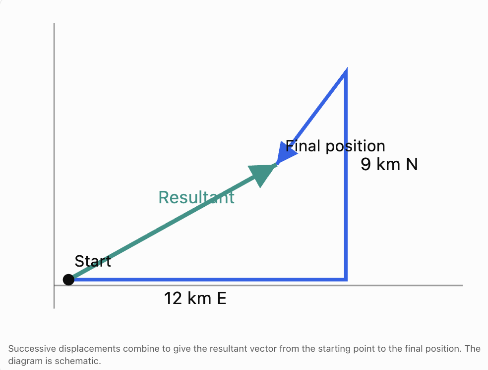
Verification
The horizontal displacement is:
12 − 3 = 9 km east.
The vertical displacement is:
9 − 4 = 5 km north.
Both components agree with the resultant vector.
Integrated Problem 2: Forces and Equilibrium
A sign with weight 120 N hangs from two cables.
The left cable makes an angle of 30° above the horizontal.
The right cable makes an angle of 60° above the horizontal.
Determine the tension in each cable.
Step 1: Define the Unknowns
Let:
T₁ = tension in the left cable.
T₂ = tension in the right cable.
The sign is stationary, so the net force is zero.
Step 2: Resolve Horizontal Forces
The horizontal components must balance:
Therefore:
Multiplying by 2:
Step 3: Resolve Vertical Forces
The upward forces must balance the weight:
Therefore:
Multiplying by 2:
Step 4: Express as a Matrix Equation
Step 5: Solve the System
From the first equation:
Substitute:
Then:
Step 6: Verify
Horizontal components:
Vertical components:
Both equilibrium conditions are satisfied.
Interpretation
The right cable has greater tension because it provides a larger share of the upward force.
This problem integrates vector resolution, trigonometry, matrix representation, and simultaneous equations.
Integrated Problem 3: Solving an Engineering System
An electrical network is modelled by three simultaneous equations:
where I₁, I₂, and I₃ are currents measured in amperes.
Find the three currents.
Step 1: Construct the Matrix Equation
where:
Step 2: Use Substitution or Elimination
From the first equation:
From the third:
Therefore:
Substitute into the middle equation:
Using I₂ = 3I₃ − 5:
Then:
And:
Final Answer
Approximately:
I₁ = 3.13 A
I₂ = 2.40 A
I₃ = 2.47 A
Verification
First equation:
Second equation:
Third equation:
All equations are satisfied.
Integrated Problem 4: Determinants and Inverse Matrices
Consider the matrix:
We want to determine whether A is invertible and use it to solve:
Step 1: Calculate the Determinant
For a 2 × 2 matrix:
Therefore:
Since the determinant is nonzero, A is invertible.
Step 2: Find the Inverse
Step 3: Solve
Step 4: Verify
The solution is correct.
Choosing an Efficient Method
For a single system, Gaussian elimination is often more efficient than calculating the inverse explicitly.
However, the inverse is useful when investigating the transformation itself or when studying how solutions depend on different right-hand-side vectors.
Integrated Problem 5: Geometric Transformations
A triangle has vertices:
A(1, 1)
B(3, 1)
C(2, 3)
It undergoes the following transformations:
-
Reflection in the y-axis.
-
Rotation of 90° anticlockwise about the origin.
-
Enlargement by scale factor 2.
Determine the final coordinates.
Step 1: Reflection Matrix
Reflection in the y-axis:
Step 2: Rotation Matrix
A 90° anticlockwise rotation:
Step 3: Enlargement Matrix
Scale factor 2:
Step 4: Combine the Transformations
The transformations are applied in the order:
Reflection, rotation, enlargement.
Therefore:
First:
Then:
Step 5: Transform Each Vertex
For any point:
Therefore:
For A(1, 1):
A′(−2, −2)
For B(3, 1):
B′(−2, −6)
For C(2, 3):
C′(−6, −4)
Final Answer
Step 6: Verify Using the Determinant
The absolute determinant is 4.
Therefore, areas are multiplied by 4.
The negative sign indicates a reversal of orientation.
This is consistent with the reflection.
Integrated Problem 6: Eigenvalues and Long-Term Behaviour
Consider a system described by:
where:
The matrix represents movement between two categories.
Each column sums to 1, so A is a column-stochastic transition matrix.
Suppose:
Step 1: Calculate the First State
Step 2: Calculate the Second State
Step 3: Find the Steady State
A steady-state vector satisfies:
Therefore:
Let:
Then:
Therefore:
The total population is 100:
Final Answer
The system approaches a steady-state distribution of 60 in the first category and 40 in the second.
Interpretation
The steady-state vector is an eigenvector associated with eigenvalue 1.
The other eigenvalue is 0.5, so deviations from the steady state decrease over time.
This connects matrix multiplication, eigenvalues, eigenvectors, and mathematical modelling.
Integrated Problem 7: Data Science and Least Squares
A scientist measures how a quantity y changes with x.
The observations are:
|
x |
y |
|---|---|
|
1 |
3 |
|
2 |
5 |
|
3 |
7 |
The scientist wants to fit a linear model:
Step 1: Construct the Design Matrix
The parameter vector is:
The observation vector is:
Step 2: Form the Normal Equations
Calculate:
and:
Therefore:
Step 3: Solve
The equations are:
Multiply the second equation by 2:
Subtract:
Then:
Final Model
Step 4: Verify
For x = 1:
y = 3
For x = 2:
y = 5
For x = 3:
y = 7
All observations lie exactly on the fitted line.
The residuals are all zero.
Therefore:
This example integrates matrices, simultaneous equations, and statistical modelling.
Integrated Problem 8: Optimisation and Resource Allocation
A company produces two products.
Product A earns $30 profit per unit.
Product B earns $50 profit per unit.
The constraints are:
Find the maximum profit.
Step 1: Write the Objective Function
Step 2: Determine the Vertices
The feasible region has vertices:
(0, 0)
(50, 0)
(0, 40)
and the intersection of:
2x + y = 100
x + 2y = 80
Solving gives:
Step 3: Evaluate the Objective
|
Vertex |
Profit |
|---|---|
|
(0, 0) |
$0 |
|
(50, 0) |
$1,500 |
|
(0, 40) |
$2,000 |
|
(40, 20) |
$2,200 |
Final Answer
Interpretation
The company should produce 40 units of A and 20 units of B.
Both constraints are active at the optimum:
The solution is feasible and maximises the linear objective.
Integrated Problem 9: Three-Dimensional Geometry
Consider the vectors:
Find:
-
Their dot product.
-
The angle between them.
-
Their cross product.
-
The area of the parallelogram they form.
Step 1: Dot Product
Therefore, the vectors are perpendicular.
Step 2: Angle
Since the dot product is zero:
Step 3: Cross Product
Calculate:
Step 4: Parallelogram Area
The parallelogram has an area of approximately 17.15 square units.
Verification
Because the vectors are perpendicular:
Therefore:
Both methods agree.
Integrated Problem 10: A Mathematical Modelling Investigation
A delivery drone must travel from a warehouse to a destination.
The destination is located:
-
6 km east.
-
8 km north.
A steady wind produces a velocity of:
The drone must arrive in exactly 1 hour.
Determine the required air-velocity vector and its magnitude.
Step 1: Define the Required Ground Velocity
The displacement vector is:
Since the journey takes 1 hour:
Step 2: Relate Ground Velocity, Air Velocity, and Wind
Therefore:
Step 3: Calculate Air Velocity
Step 4: Calculate Airspeed
Step 5: Calculate Heading
The drone must head approximately 41.2° north of east relative to the air.
Step 6: Verify
Over one hour, this produces the required displacement.
Model Evaluation
This solution assumes:
-
Wind velocity is constant.
-
The drone maintains a constant air velocity.
-
The route is unobstructed.
-
Acceleration and takeoff time are negligible.
-
The drone can maintain the required airspeed.
A more realistic model might include changing wind, energy consumption, battery limits, and flight restrictions.
Mathematical Communication and Justification
A complete mathematical solution should communicate more than a final number.
A strong solution contains:
-
Clearly defined variables.
-
Appropriate mathematical representations.
-
A justified choice of method.
-
Correct algebraic or numerical working.
-
Suitable units.
-
Verification of results.
-
Interpretation in context.
-
Recognition of assumptions and limitations.
Example: Weak and Strong Communication
Weak response:
x = 40, y = 20.
Stronger response:
Let x and y represent the numbers of units of Products A and B. The objective is to maximise P = 30x + 50y subject to the production constraints. Evaluating the objective at the feasible vertices gives the maximum profit of $2,200 at (40, 20). Therefore, the company should produce 40 units of A and 20 units of B. Both resource constraints are satisfied with equality.
The second response explains the meaning of the variables, the mathematical method, the result, and its interpretation.
Common Mistakes
Mistake 1: Choosing a method before understanding the problem
Always identify the mathematical structure before deciding on a technique.
Mistake 2: Confusing scalar and vector quantities
Vectors have magnitude and direction, while scalars have magnitude only.
Mistake 3: Adding vectors without considering direction
Vector components must be added using a consistent coordinate system.
Mistake 4: Using the wrong matrix multiplication order
In general:
AB ≠ BA
For column vectors, the rightmost transformation matrix acts first.
Mistake 5: Assuming every square matrix is invertible
A matrix is invertible only when its determinant is nonzero.
Mistake 6: Using an inverse without checking dimensions
The inverse method requires an appropriate square, invertible coefficient matrix.
Mistake 7: Confusing dot products and cross products
A dot product produces a scalar. A three-dimensional cross product produces a vector.
Mistake 8: Misinterpreting eigenvectors
Eigenvectors retain their direction or line under a transformation, but may change magnitude or reverse orientation.
Mistake 9: Forgetting constraints in optimisation
An unconstrained solution may not be feasible.
Mistake 10: Assuming numerical results are automatically meaningful
A mathematical solution must be interpreted in the original context.
Mistake 11: Rounding too early
Keep exact values or sufficient decimal precision during intermediate calculations.
Mistake 12: Failing to verify solutions
Substitution and alternative methods help identify mistakes.
Mistake 13: Ignoring units
Physical quantities must be reported using appropriate units.
Mistake 14: Confusing local and global solutions
A local optimum may not be the best solution over the entire feasible region.
Mistake 15: Presenting answers without justification
Mathematical communication should explain why the method works and what the result means.
Key Terms
-
Vector: Quantity represented by magnitude and direction, or more generally an element of a vector space.
-
Scalar: Single numerical quantity.
-
Component: Coordinate of a vector along a specified axis.
-
Resultant Vector: Vector obtained by combining two or more vectors.
-
Magnitude: Length or size of a vector.
-
Unit Vector: Vector with magnitude 1.
-
Dot Product: Scalar obtained from corresponding vector components.
-
Cross Product: Vector perpendicular to two three-dimensional vectors.
-
Projection: Component of one vector along another direction.
-
Matrix: Rectangular arrangement of numerical entries.
-
Matrix Multiplication: Operation combining rows and columns of compatible matrices.
-
Transpose: Matrix obtained by interchanging rows and columns.
-
Determinant: Scalar associated with a square matrix that indicates invertibility and geometric scaling.
-
Inverse Matrix: Matrix that reverses the effect of an invertible matrix.
-
Identity Matrix: Matrix that leaves vectors unchanged under multiplication.
-
Gaussian Elimination: Method of solving linear systems using row operations.
-
Rank: Number of linearly independent rows or columns of a matrix.
-
Linear Independence: Condition where no vector in a collection can be formed as a linear combination of the others.
-
Basis: Linearly independent set of vectors spanning a vector space.
-
Eigenvalue: Scalar describing how an eigenvector is scaled by a transformation.
-
Eigenvector: Nonzero vector whose direction remains along the same line under a linear transformation.
-
Transformation Matrix: Matrix representing a linear transformation.
-
Composite Transformation: Combination of two or more transformations.
-
Equilibrium: State in which the resultant force is zero.
-
Steady State: State unchanged by repeated application of a transition model.
-
Transition Matrix: Matrix describing movement between states.
-
Least Squares: Method that minimises the sum of squared residuals.
-
Residual: Difference between an observed and predicted value.
-
Optimisation: Process of finding the best value of an objective.
-
Objective Function: Function to be maximised or minimised.
-
Constraint: Restriction on possible solutions.
-
Feasible Region: Set of all solutions satisfying the constraints.
-
Mathematical Model: Mathematical representation of a real system.
-
Verification: Process of checking whether a result satisfies the original conditions.
-
Mathematical Justification: Explanation showing why a method or conclusion is valid.
Key Takeaways
-
Complex problems often require several mathematical concepts to be combined.
-
The first step is to understand the problem and identify the relevant variables.
-
Vectors are useful for representing displacement, velocity, force, and other multicomponent quantities.
-
Dot products help calculate angles, projections, and physical work.
-
Cross products help calculate perpendicular directions, areas, and moments.
-
Matrices provide compact representations of simultaneous equations and transformations.
-
Gaussian elimination is a versatile method for solving linear systems.
-
Determinants help determine whether square matrices are invertible.
-
Matrix multiplication allows transformations to be combined.
-
The order of transformations matters.
-
Eigenvalues and eigenvectors describe important properties of repeated linear transformations.
-
Matrix models are useful for analysing systems that evolve over time.
-
Least-squares methods use matrices to fit mathematical models to data.
-
Optimisation identifies the best feasible solution to a mathematical problem.
-
Efficient problem solving involves selecting methods suited to the mathematical structure.
-
Verification is essential for detecting errors and confirming results.
-
Mathematical communication should include definitions, reasoning, calculations, and interpretations.
-
Real-world models must be evaluated for assumptions, limitations, and practical usefulness.
Check Your Understanding
Questions
Question 1: Vector Addition
Given:
and:
Calculate 2a + b.
Question 2: Resultant Displacement
A person walks 8 km east and 6 km north.
Calculate the magnitude and direction of the resultant displacement.
Question 3: Dot Product
Given:
and:
Calculate their dot product and determine the angle between them.
Question 4: Cross Product
Calculate:
Question 5: Matrix Multiplication
Calculate:
Question 6: Determinants
Calculate the determinant of:
Determine whether A is invertible.
Question 7: Inverse Matrix
Find the inverse of:
Question 8: Solving Systems
Solve:
Question 9: Geometric Transformations
A point P(2, 3) is reflected in the x-axis and then rotated 90° anticlockwise.
Find its final coordinates.
Question 10: Eigenvalues
Find the eigenvalues of:
Question 11: Matrix Modelling
Given:
and:
Calculate the next state.
Question 12: Least Squares
A model predicts:
5, 7, 9
Actual observations are:
6, 8, 8
Calculate the sum of squared errors.
Question 13: Optimisation
Maximise:
subject to:
Question 14: Engineering Equilibrium
Two horizontal forces act on an object:
Find the third force required for equilibrium.
Question 15: Comprehensive Integrated Challenge
A robot operates in a two-dimensional coordinate system.
Its initial position is:
The robot performs the following operations:
-
Rotates 90° anticlockwise about the origin.
-
Enlarges its position vector by scale factor 2.
-
Moves 4 units east and 3 units north.
a) Write the rotation matrix.
b) Write the scaling matrix.
c) Calculate the composite linear transformation matrix.
d) Find the position after the first two transformations.
e) Find the final position after translation.
f) Calculate the distance from the origin to the final position.
g) Explain why translation cannot be represented by a standard 2 × 2 linear transformation matrix.
h) Explain how homogeneous coordinates could represent all three transformations using matrices.
Fully Worked Answers
Answer 1: Vector Addition
Answer 2: Resultant Displacement
The resultant vector is:
Magnitude:
Direction:
The displacement is 10 km at 36.9° north of east.
Answer 3: Dot Product
Since both vectors are nonzero and their dot product is zero, they are perpendicular.
Answer 4: Cross Product
Let:
Then:
Answer 5: Matrix Multiplication
First row:
2(1) + 1(0) = 2
2(2) + 1(3) = 7
Second row:
3(1) + 4(0) = 3
3(2) + 4(3) = 18
Therefore:
Answer 6: Determinants
Since the determinant is nonzero, A is invertible.
Answer 7: Inverse Matrix
Determinant:
Therefore:
Answer 8: Solving Systems
Given:
From the first equation:
Substitute:
Then:
Answer 9: Geometric Transformations
Initial point:
P(2, 3)
Reflection in the x-axis:
Therefore:
P′(2, −3)
Rotation 90° anticlockwise:
Therefore:
Answer 10: Eigenvalues
For a diagonal matrix, the eigenvalues are its diagonal entries.
Therefore:
Answer 11: Matrix Modelling
First component:
0.7(60) + 0.2(40) = 42 + 8 = 50
Second component:
0.3(60) + 0.8(40) = 18 + 32 = 50
Therefore:
Answer 12: Least Squares
Actual values:
6, 8, 8
Predicted values:
5, 7, 9
Residuals:
6 − 5 = 1
8 − 7 = 1
8 − 9 = −1
Square:
1, 1, 1
Therefore:
Answer 13: Optimisation
Objective:
Constraints:
The feasible vertices are:
(0, 0)
(5, 0)
(5, 3)
(2, 6)
(0, 6)
Evaluate:
|
Vertex |
P |
|---|---|
|
(0, 0) |
0 |
|
(5, 0) |
20 |
|
(5, 3) |
29 |
|
(2, 6) |
26 |
|
(0, 6) |
18 |
Therefore:
at:
Answer 14: Engineering Equilibrium
For equilibrium:
Therefore:
Calculate:
Therefore:
Its magnitude is:
Answer 15: Comprehensive Integrated Challenge
Initial position:
Part a: Rotation matrix
A 90° anticlockwise rotation is:
Part b: Scaling matrix
Scale factor 2:
Part c: Composite matrix
Rotation occurs first, followed by scaling.
Therefore:
Part d: Position after rotation and scaling
Part e: Final position after translation
Translation vector:
Therefore:
Final position:
Part f: Distance from the origin
Part g: Why translation cannot be represented by a standard 2 × 2 matrix
A linear transformation must map the zero vector to the zero vector.
However, a translation moves the origin:
Therefore, a nonzero translation is not a linear transformation in ordinary two-dimensional coordinates.
Part h: Homogeneous coordinates
Homogeneous coordinates add a third coordinate:
The rotation, scaling, and translation can be combined into a single 3 × 3 matrix:
Apply H to the initial point:
This confirms the final position:
Final Reflection
Vectors and matrices provide a unified mathematical language for solving problems across mathematics, physics, engineering, economics, computer science, and artificial intelligence.
Vector operations describe movement, forces, geometry, and spatial relationships. Matrix methods allow simultaneous equations, transformations, and dynamic systems to be represented and solved efficiently. Determinants, inverses, eigenvalues, and eigenvectors reveal deeper structural properties of mathematical systems.
More advanced applications combine these ideas with statistics, calculus, optimisation, and mathematical modelling.
The most important skill is not simply performing calculations correctly. It is recognising the structure of a problem, choosing an appropriate method, explaining the reasoning, checking the solution, and interpreting the result.
Successful comprehensive problem solving requires mathematical knowledge, logical reasoning, efficient strategy selection, and clear communication.