Matrix Transformations and Applications

Introduction

Matrices are among the most useful mathematical tools in science and engineering. They allow scientists and engineers to organise large amounts of information, describe relationships between variables, solve simultaneous equations, and predict how physical systems will behave.

Consider some important questions:

• How can engineers calculate the forces acting on a bridge?

• How can electrical engineers determine currents in a complicated circuit?

• How can scientists analyse measurements from several experiments?

• How can engineers predict the movement of a mechanical system?

• How can environmental scientists model the movement of pollutants?

• How can researchers use data to identify relationships between physical quantities?

Although these problems involve different scientific disciplines, many can be represented using the same mathematical structure:

where:

• A is a matrix containing the relationships between variables.

• x is a vector containing unknown quantities.

• b is a vector containing known values.

Once a problem has been represented using matrices, mathematical methods can be used to calculate unknown quantities, analyse relationships, and evaluate possible solutions.

In this lesson, we will explore how matrices are applied to engineering systems, mechanics, electrical circuits, scientific data, population models, and other authentic STEM problems.

Why Matrices Are Important in STEM

Scientific and engineering problems often involve several variables that interact with one another.

For example, the movement of an object may depend on:

• Position

• Velocity

• Acceleration

• Applied forces

• Mass

• Time

An electrical circuit may involve:

• Voltage

• Current

• Resistance

• Multiple branches

• Several connected components

A matrix provides an organised way to represent these relationships.

The General Matrix Model

Consider the simultaneous equations:

2x + 3y = 12

4x − y = 5

These can be written as:

Or:

The coefficient matrix is:

The unknown vector is:

The known vector is:

If A is invertible:

For larger systems, engineers usually use numerical methods such as matrix factorisation rather than calculating the inverse explicitly.

Worked Example 1: Solving an Engineering System

Solve:

3x + 2y = 16

x + 4y = 12

Write the matrix equation:

Calculate the determinant:

det(A) = 3(4) − 2(1) = 10

The inverse is:

Therefore:

Therefore:

Verify:

3(4) + 2(2) = 16

4 + 4(2) = 12

Both equations are satisfied.

Matrices in Structural Engineering

Structural engineers analyse buildings, bridges, towers, and other structures to ensure they can support applied forces.

Forces may include:

• The weight of the structure.

• The weight of people and vehicles.

• Wind loads.

• Earthquake forces.

• Tension and compression in structural members.

A structure must satisfy the conditions of equilibrium.

For a stationary object in two dimensions:

For a rigid body, rotational equilibrium is also required:

These equations can be combined into matrix form.

Worked Example 2: Forces in Two Supporting Cables

A 100 N load is supported by two cables.

Cable A makes an angle of 30° above the horizontal.

Cable B makes an angle of 60° above the horizontal on the opposite side.

Find the tension in each cable.

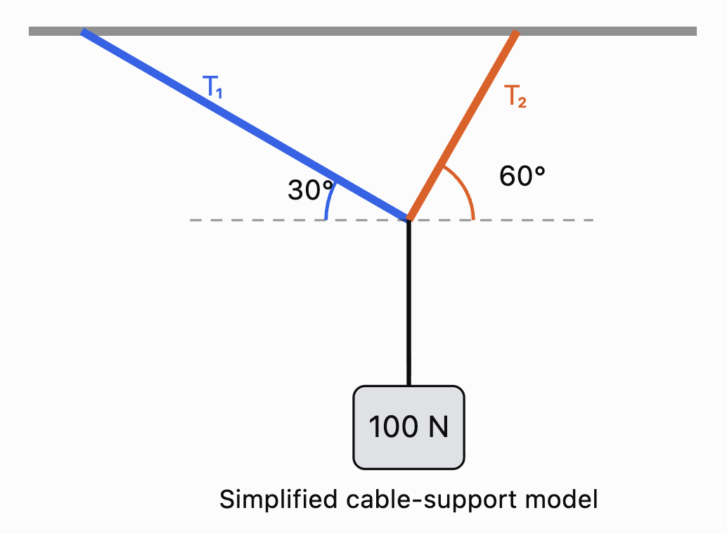
Let:

T₁ = tension in Cable A

T₂ = tension in Cable B

Step 1: Horizontal Equilibrium

The horizontal forces must balance.

Rearrange:

Step 2: Vertical Equilibrium

The upward forces must equal the weight.

Step 3: Write the Matrix Equation

Substitute approximate trigonometric values:

Step 4: Solve

From the horizontal equation:

0.866T₁ = 0.5T₂

Therefore:

T₂ ≈ 1.732T₁

Substitute into the vertical equation:

0.5T₁ + 0.866(1.732T₁) = 100

0.5T₁ + 1.5T₁ = 100

2T₁ = 100

T₁ = 50 N

Then:

T₂ ≈ 1.732(50)

T₂ ≈ 86.6 N

Therefore:

Interpretation

The cable at 60° has the greater tension.

The two cables together provide sufficient upward force to support the 100 N load while their horizontal components cancel.

Matrix methods become particularly valuable when a structure contains many connected members and unknown forces.

Matrices in Electrical Engineering

Electrical engineers use matrices to analyse circuits containing multiple resistors, voltage sources, and branches.

Two important principles are:

Ohm's Law

where:

• V = voltage (V)

• I = current (A)

• R = resistance (Ω)

Kirchhoff's Voltage Law

The algebraic sum of voltage changes around a closed loop is zero.

Kirchhoff's Current Law states that the total current entering a junction equals the total current leaving it.

These laws produce systems of linear equations that can be solved using matrices.

Worked Example 3: A Two-Loop Circuit

Consider two adjacent circuit loops sharing a resistor.

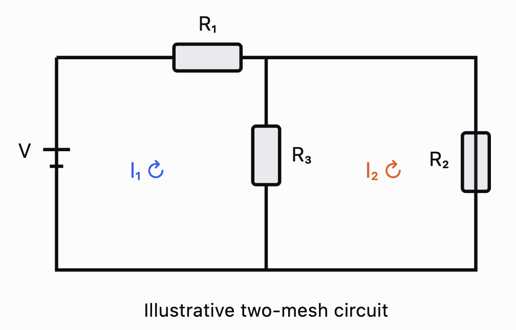
Suppose the mesh-current equations obtained from Kirchhoff's laws are:

5I₁ − 2I₂ = 12

−2I₁ + 6I₂ = 6

Here, the coefficients represent resistances in ohms and the constants represent voltages.

Write the system as:

Step 1: Calculate the Determinant

det(A) = 5(6) − (−2)(−2)

= 30 − 4

= 26

Step 2: Calculate the Inverse

Step 3: Solve for the Currents

Therefore:

Interpretation

The two mesh currents are approximately 3.23 A and 2.08 A.

If the mesh currents pass through the shared resistor in opposite directions, the current through that resistor is:

I₁ − I₂ ≈ 1.15 A

The matrix method provides an organised way to calculate multiple currents simultaneously.

Matrices in Mechanical Engineering

Mechanical engineers use matrices to model systems involving forces, motion, deformation, and vibration.

A common example is a system of masses connected by springs.

Hooke's Law

For an ideal spring:

where:

• F = restoring force

• k = spring constant

• x = displacement from equilibrium

The negative sign indicates that the restoring force acts opposite to the displacement.

Coupled Spring Systems

Suppose two movable masses are connected to fixed walls and to each other by springs.

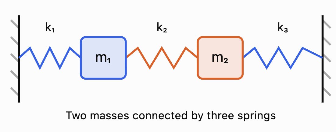
Let:

x₁ = displacement of Mass 1

x₂ = displacement of Mass 2

If the system is displaced slightly from equilibrium, the restoring-force equations can be written:

In matrix form:

where:

and:

M is called the mass matrix.

K is called the stiffness matrix.

This matrix equation describes how the masses move together.

It is important in the study of:

• Vehicle suspension systems.

• Building vibrations.

• Earthquake engineering.

• Mechanical resonance.

• Aircraft structures.

• Industrial machinery.

Worked Example 4: Static Spring Displacements

Consider a simplified spring system whose static equilibrium is described by:

The stiffness coefficients are measured in N/m, the applied forces in N, and the displacements in m.

This gives:

30x₁ − 10x₂ = 50

−10x₁ + 20x₂ = 20

Divide both equations by 10:

3x₁ − x₂ = 5

−x₁ + 2x₂ = 2

From the first equation:

x₂ = 3x₁ − 5

Substitute into the second:

−x₁ + 2(3x₁ − 5) = 2

−x₁ + 6x₁ − 10 = 2

5x₁ = 12

x₁ = 2.4

Then:

x₂ = 3(2.4) − 5

x₂ = 2.2

Therefore:

These are the displacements predicted by the ideal linear spring model.

In a real engineering application, such large displacements might exceed the range where Hooke's law is valid. Engineers would need to check whether the model's assumptions remain reasonable.

Matrices in Scientific Data Analysis

Scientists frequently collect measurements from experiments.

Matrices allow data to be organised and analysed efficiently.

Suppose an experiment measures the temperature and pressure of a gas at several times.

The data can be represented by:

Each row represents an observation.

Each column represents a measured variable.

Matrices are particularly useful when datasets contain many observations and several variables.

Data Transformations

Suppose all temperatures must be converted from kelvin to degrees Celsius.

The conversion is:

°C = K − 273.15

The temperature column can be transformed by subtracting 273.15 from each entry.

More generally, data can be transformed using matrix operations to:

• Change units.

• Centre variables around their means.

• Standardise measurements.

• Combine datasets.

• Calculate predictions.

• Identify patterns.

Matrices and Linear Regression

One of the most important applications of matrices in scientific data analysis is linear regression.

Linear regression finds a mathematical relationship between variables.

Suppose we believe the relationship between two quantities is approximately linear:

where:

• m = gradient

• c = intercept

If several measurements are available, we can construct a matrix equation.

For observations (x₁, y₁), (x₂, y₂), ..., (xₙ, yₙ):

The unknown parameter vector is:

The observed values are:

We model:

The least-squares solution minimises the sum of squared residuals.

When X has full column rank:

This formula is called the normal-equation solution.

For numerical work, QR factorisation or other stable methods are often preferred over explicitly forming the inverse.

Worked Example 5: Finding a Line of Best Fit

A student measures the extension of a spring under different forces.

We want to model:

y = mx + c

Construct:

and:

Calculate:

Also:

The normal equations are:

This gives:

14m + 6c = 25

6m + 3c = 11

Multiply the second equation by 2:

12m + 6c = 22

Subtract:

2m = 3

m = 1.5

Substitute:

6(1.5) + 3c = 11

9 + 3c = 11

c = 2/3

Therefore:

The model predicts an extension of approximately 1.5 cm for every additional newton of force, with an intercept of approximately 0.667 cm.

In a perfectly calibrated Hooke's law experiment, extension would be expected to be zero at zero applied force. The nonzero intercept may reflect measurement error, a zero offset, or limitations in the data.

Visualising Scientific Regression

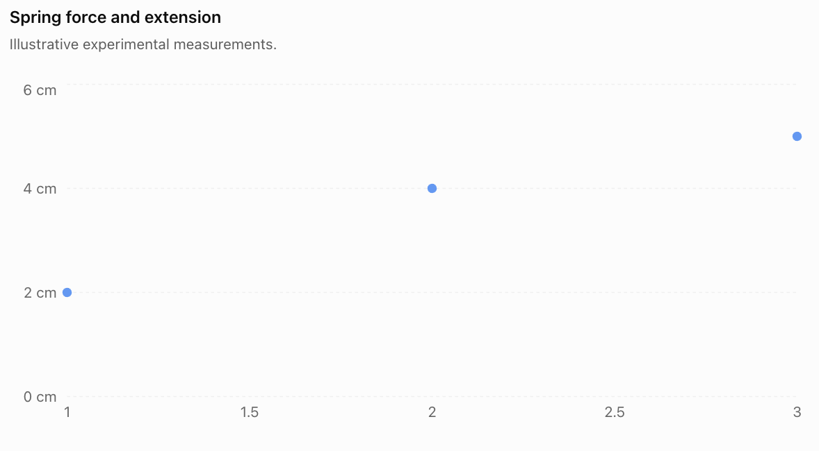
The matrix regression model allows scientists to estimate a relationship even when measurements do not lie exactly on a straight line.

This is useful because real experimental data almost always contains uncertainty.

Matrices in Population and Environmental Science

Matrices can also model how populations change over time.

Suppose a population contains two age groups:

• Juveniles

• Adults

The number of individuals in each group can be represented by a population vector:

where:

• Jₙ = number of juveniles at time n.

• Aₙ = number of adults at time n.

A transition matrix describes survival, reproduction, and movement between age groups.

Worked Example 6: Population Growth

Suppose:

• Each adult produces an average of 2 juveniles per year.

• 50% of juveniles survive to become adults.

• 80% of adults survive into the following year.

• Juveniles do not remain in the juvenile category after one year.

The population matrix is:

Initially, there are:

100 juveniles

50 adults

Therefore:

The next year's population is:

Juveniles:

0(100) + 2(50) = 100

Adults:

0.5(100) + 0.8(50) = 90

Therefore:

After one year, the model predicts:

• 100 juveniles

• 90 adults

Total population = 190

Predicting the Second Year

Juveniles:

0(100) + 2(90) = 180

Adults:

0.5(100) + 0.8(90) = 122

Therefore:

Total population = 302

Interpretation

The model predicts population growth.

However, this does not guarantee that the real population will continue increasing indefinitely.

The model assumes constant reproduction and survival rates and does not account for limited food, disease, competition, or environmental changes.

Notice that this is not a probability transition matrix: the first column and second column do not both sum to 1. Reproduction can add new individuals, so total population is not necessarily conserved.

Matrices in Chemical Engineering

Chemical engineers use matrices to model chemical reactions, material flows, and industrial production processes.

One important application is balancing chemical equations.

Representing Chemical Reactions with Matrices

Consider the combustion of methane:

CH₄ + O₂ → CO₂ + H₂O

Let the unknown coefficients be:

aCH₄ + bO₂ → cCO₂ + dH₂O

Conservation of atoms gives three equations.

Carbon:

a − c = 0

Hydrogen:

4a − 2d = 0

Oxygen:

2b − 2c − d = 0

These can be represented as:

This is a homogeneous system of linear equations.

Worked Example 7: Balancing a Chemical Equation

From carbon conservation:

a = c

From hydrogen conservation:

4a = 2d

Therefore:

d = 2a

From oxygen conservation:

2b = 2c + d

Substitute c = a and d = 2a:

2b = 2a + 2a

2b = 4a

b = 2a

Choose the smallest positive integer value:

a = 1

Then:

b = 2

c = 1

d = 2

Therefore:

Why Matrices Are Useful

For simple chemical reactions, balancing by inspection is often faster.

However, complicated chemical reactions may contain many elements and compounds.

Matrix methods allow the conservation equations to be organised and solved systematically.

This is especially useful in chemical engineering software and reaction-network modelling.

Matrices in Computer Science and Engineering

Matrices are used extensively in computing, particularly in graphics, machine learning, image processing, and robotics.

A digital image can be represented as a matrix of pixel values.

For a grayscale image, each matrix entry represents the brightness of a pixel.

For example:

Here, pixel values range from 0 to 255.

• 0 represents black.

• 255 represents white.

• Intermediate values represent shades of gray.

  

  Matrix operations can be used to:

  • Increase or decrease brightness.

  • Rotate and resize images.

  • Detect edges.

  • Reduce noise.

  • Apply filters.

  • Analyse image patterns.

  Worked Example 8: Increasing Image Brightness

  Suppose an image has pixel matrix:

  \[ I=\begin{bmatrix} 50&100\\ 150&200 \end{bmatrix} \]

  We want to increase every pixel value by 30.

  Add:

  \[ B=\begin{bmatrix} 30&30\\ 30&30 \end{bmatrix} \]

  Then:

  \[ I'=I+B \]

  \[ I'= \begin{bmatrix} 80&130\\ 180&230 \end{bmatrix} \]

  Therefore:

  \[ \boxed{ I'=\begin{bmatrix} 80&130\\ 180&230 \end{bmatrix} } \]

  The image becomes brighter.

  If a calculation produces a value above 255, an 8-bit image-processing system must handle the value appropriately, often by clipping it to 255.

   

  Matrices in Fluid Flow and Environmental Modelling

  Environmental scientists and engineers use matrices to model the movement of water, air, pollutants, and other substances.

  Suppose a lake is divided into two regions.

  Each day:

  • 80% of the pollutant in Region A remains there.

  • 20% moves from A to B.

  • 10% of the pollutant in Region B moves to A.

  • 90% remains in B.

  The transition matrix is:

  \[ T=\begin{bmatrix} 0.8&0.1\\ 0.2&0.9 \end{bmatrix} \]

  Suppose initially:

  Region A contains 100 kg of pollutant.

  Region B contains 50 kg.

  Then:

  \[ \mathbf{P}_0=\begin{bmatrix}100\\50\end{bmatrix} \]

  Worked Example 9: Pollutant Movement

  Calculate:

  \[ \mathbf{P}_1=T\mathbf{P}_0 \]

  \[ \mathbf{P}_1= \begin{bmatrix} 0.8&0.1\\ 0.2&0.9 \end{bmatrix} \begin{bmatrix} 100\\50 \end{bmatrix} \]

  Region A:

  0.8(100) + 0.1(50)

  = 80 + 5

  = 85 kg

  Region B:

  0.2(100) + 0.9(50)

  = 20 + 45

  = 65 kg

  Therefore:

  \[ \boxed{\mathbf{P}_1=\begin{bmatrix}85\\65\end{bmatrix}\text{ kg}} \]

  The total remains:

  85 + 65 = 150 kg

  This is consistent with the model's assumption that pollutant moves between regions but is not created or destroyed.

  Model Limitations

  The model does not include:

  • Chemical decomposition.

  • Evaporation.

  • New pollution sources.

  • Changes in water flow.

  • Seasonal weather patterns.

  • Pollutant absorption by sediments or organisms.

  A more advanced model could include additional regions and processes.

   

  Analysing and Interpreting Matrix Models

  A mathematical model is useful only when its results can be interpreted meaningfully.

  Scientists and engineers must consider several important questions.

  Are the Units Consistent?

  Suppose a stiffness matrix is measured in N/m and a displacement vector is measured in m.

  Then:

  \[ K\mathbf{x}=\mathbf{F} \]

  The units are:

  (N/m) × m = N

  This produces a force vector, as expected.

  Dimensional analysis helps identify errors in scientific models.

  Does the Solution Make Physical Sense?

  A mathematical solution may be correct but physically impossible.

  Examples include:

  • A negative mass.

  • A probability greater than 1.

  • A robotic arm reaching beyond its maximum length.

  • A structural member carrying a force beyond its safe capacity.

  • A predicted temperature outside the model's valid range.

  Solutions must be checked against physical constraints.

  Is the Model Sensitive to Changes?

  A model may be highly sensitive to small changes in its inputs.

  For example, a small measurement error may produce a large change in the calculated solution if the coefficient matrix is nearly singular.

  The condition number of a matrix is one measure of this sensitivity.

  A large condition number indicates that small errors in the data may cause relatively large errors in the calculated solution.

  Is the Model Appropriate?

  A linear matrix model may work well for small changes but fail for larger changes.

  For example:

  • Springs may stop obeying Hooke's law.

  • Air resistance may depend nonlinearly on speed.

  • Population growth may be limited by resources.

  • Material properties may change with temperature.

  Scientists must choose models appropriate to the situation.

   

  Sensitivity Analysis: An Engineering Example

  Consider the system:

  \[ \begin{bmatrix} 1&1\\ 1&1.01 \end{bmatrix} \begin{bmatrix} x\\y \end{bmatrix} = \begin{bmatrix} 2\\2.01 \end{bmatrix} \]

  The equations are:

  x + y = 2

  x + 1.01y = 2.01

  Subtract the first equation from the second:

  0.01y = 0.01

  y = 1

  Therefore:

  x = 1

  The solution is:

  \[ \boxed{(x,y)=(1,1)} \]

  Now suppose the second measured value changes slightly from 2.01 to 2.02.

  The new system is:

  x + y = 2

  x + 1.01y = 2.02

  Subtract:

  0.01y = 0.02

  y = 2

  Then:

  x = 0

  The new solution is:

  \[ \boxed{(x,y)=(0,2)} \]

  A change of only 0.01 in the measured value produced a large change in the solution.

  This happens because the equations are nearly dependent.

  The example demonstrates why scientists and engineers must consider measurement uncertainty and numerical sensitivity.

   

  Choosing the Correct Matrix Method

  Different STEM problems require different matrix techniques.

  Problem	Matrix technique
  Simultaneous engineering equations	Gaussian elimination or matrix factorisation
  Small invertible linear systems	Inverse matrix
  Structural force calculations	Equilibrium equations in matrix form
  Electrical circuits	Kirchhoff's laws and linear systems
  Spring and vibration systems	Mass and stiffness matrices
  Scientific regression	Least squares
  Population growth	Matrix recurrence models
  Chemical equation balancing	Null space of a matrix
  Image processing	Matrix and array operations
  Environmental transport	Transition and flow matrices
  Stability of dynamic systems	Eigenvalues and eigenvectors

  The appropriate method depends on the mathematical structure of the problem.

  A key skill in applied mathematics is recognising which matrix method best represents the situation.

   

  Common Mistakes

  Mistake 1: Constructing the matrix incorrectly

  Rows and columns must represent the intended variables and relationships. Incorrect placement of coefficients produces incorrect results.

  Mistake 2: Ignoring the order of matrix multiplication

  In general, AB ≠ BA. The order must reflect the physical or mathematical process.

  Mistake 3: Forgetting units

  A numerical answer without appropriate units may be meaningless in an engineering context.

  Mistake 4: Assuming every matrix has an inverse

  A matrix must be square and nonsingular to have an inverse.

  Mistake 5: Using an inverse when a more suitable method is available

  Large engineering systems are generally solved using numerical factorisation methods rather than explicitly calculating inverse matrices.

  Mistake 6: Confusing a population matrix with a probability transition matrix

  A population matrix may include reproduction and growth. Its columns do not necessarily sum to 1.

  Mistake 7: Assuming experimental measurements are exact

  Real scientific data contains measurement uncertainty and possible systematic errors.

  Mistake 8: Confusing correlation with causation

  A relationship identified using matrix regression does not automatically establish that one variable causes another.

  Mistake 9: Ignoring physical constraints

  A mathematical solution may violate real-world limits such as material strength, capacity, or conservation laws.

  Mistake 10: Treating model predictions as guaranteed outcomes

  Models depend on assumptions and available data. Predictions should be interpreted as estimates.

  Mistake 11: Ignoring numerical sensitivity

  Nearly singular matrices can produce solutions that are highly sensitive to small measurement errors.

  Mistake 12: Failing to verify results

  Solutions should be substituted into the original equations and checked against the physical situation.

   

  Key Terms

  • Mathematical Model: Mathematical representation of a real-world system.

  • Coefficient Matrix: Matrix containing the coefficients of a system of equations.

  • Variable Vector: Column vector containing unknown quantities.

  • Inverse Matrix: Matrix that reverses the effect of an invertible matrix.

  • Singular Matrix: Square matrix with determinant zero.

  • Gaussian Elimination: Method of solving linear systems using row operations.

  • Matrix Factorisation: Representation of a matrix as a product of simpler matrices.

  • Equilibrium: Condition in which net force and net torque are zero.

  • Tension: Pulling force transmitted through a cable or similar component.

  • Kirchhoff's Voltage Law: Principle that the algebraic sum of voltage changes around a closed loop is zero.

  • Kirchhoff's Current Law: Principle that total current entering a junction equals total current leaving.

  • Mesh Current: Assigned circulating current used to analyse a circuit loop.

  • Hooke's Law: Relationship between restoring force and displacement for an ideal spring.

  • Stiffness Matrix: Matrix relating displacements to forces in a linear mechanical system.

  • Mass Matrix: Matrix representing the mass properties of a mechanical system.

  • Linear Regression: Method for modelling a linear relationship between variables.

  • Least Squares: Method that minimises the sum of squared residuals.

  • Residual: Difference between an observed value and a predicted value.

  • Normal Equations: Matrix equations used to obtain a least-squares solution.

  • Population Matrix: Matrix describing survival, reproduction, or movement between population groups.

  • Homogeneous System: Linear system of the form Ax = 0.

  • Null Space: Set of vectors mapped to zero by a matrix.

  • Transition Matrix: Matrix describing changes between states.

  • Pixel Matrix: Array of numerical values representing image pixels.

  • Eigenvalue: Scalar describing how an eigenvector is scaled by a matrix.

  • Condition Number: Measure of sensitivity to errors in inputs or calculations.

  • Dimensional Analysis: Checking relationships using physical units.

  • Model Validation: Comparing model predictions with observed evidence.

  • Sensitivity Analysis: Investigating how changes in inputs affect outputs.

  • Conservation Law: Scientific principle stating that a quantity is conserved under specified conditions.

   

  Key Takeaways

  • Matrices provide an organised way to represent complex scientific and engineering systems.

  • Many STEM problems can be expressed as Ax = b.

  • Structural engineers use matrices to calculate forces and support loads.

  • Electrical engineers use matrices to solve circuit equations.

  • Mechanical engineers use mass and stiffness matrices to model motion and vibration.

  • Scientific datasets can be organised into matrices for analysis.

  • Matrix least-squares methods help determine relationships between measured variables.

  • Population matrices can model survival, reproduction, and population growth.

  • Chemical equations can be balanced using homogeneous linear systems.

  • Images can be represented and processed using matrices of pixel values.

  • Transition matrices can model the movement of pollutants between regions.

  • Eigenvalues can help analyse the stability and behaviour of physical systems.

  • Nearly singular matrices can produce solutions sensitive to measurement errors.

  • Scientific models must be interpreted using correct units, physical constraints, and realistic assumptions.

   

  Check Your Understanding

  Questions

  Question 1: Matrix Representation

  Represent the following system in matrix form:

  3x + 2y = 14

  5x − y = 8

  Question 2: Engineering Equations

  Solve the system from Question 1.

  Question 3: Structural Engineering

  A load is supported by two vertical cables carrying tensions T₁ and T₂.

  The total upward force is 200 N.

  Cable 1 carries 40 N more tension than Cable 2.

  Construct a matrix equation and calculate both tensions.

  Question 4: Electrical Engineering

  Two mesh currents satisfy:

  4I₁ − I₂ = 11

  −I₁ + 3I₂ = 7

  Calculate I₁ and I₂.

  Question 5: Spring Systems

  A mechanical system is represented by:

  \[ \begin{bmatrix} 20&-5\\ -5&15 \end{bmatrix} \begin{bmatrix} x_1\\x_2 \end{bmatrix} = \begin{bmatrix} 35\\25 \end{bmatrix} \]

  Calculate the two displacements. Assume stiffness coefficients are in N/m and forces in N.

  Question 6: Scientific Data

  A scientist records the following measurements:

  Time (s)	Distance (m)
  1	3
  2	6
  3	9

  Represent the measurements using a 3 × 2 data matrix.

  Question 7: Linear Regression

  The points (1, 2), (2, 4), and (3, 6) lie on a straight line.

  Determine the regression equation y = mx + c.

  Question 8: Population Modelling

  A population is modelled by:

  \[ L=\begin{bmatrix} 0&3\\ 0.4&0.7 \end{bmatrix} \]

  Initially:

  \[ \mathbf{P}_0=\begin{bmatrix} 50\\40 \end{bmatrix} \]

  Calculate the population after one year.

  Question 9: Chemical Engineering

  Balance the chemical equation using conservation of atoms:

  Fe + O₂ → Fe₂O₃

  Question 10: Image Processing

  An image has pixel matrix:

  \[ I=\begin{bmatrix} 40&80\\ 120&160 \end{bmatrix} \]

  Increase every pixel value by 20.

  Question 11: Environmental Modelling

  A pollutant transition matrix is:

  \[ T=\begin{bmatrix} 0.9&0.2\\ 0.1&0.8 \end{bmatrix} \]

  Initially:

  \[ \mathbf{P}_0=\begin{bmatrix} 80\\20 \end{bmatrix} \]

  Calculate the pollutant distribution after one time period.

  Question 12: Model Interpretation

  Explain why a mathematical model may produce a correct numerical solution but an unrealistic physical prediction.

  Question 13: Matrix Sensitivity

  Explain why a nearly singular coefficient matrix can be problematic when analysing experimental data.

  Question 14: Choosing Matrix Methods

  Identify an appropriate matrix technique for each situation:

  a) Calculating currents in an electrical circuit.

  b) Finding a line of best fit for experimental measurements.

  c) Predicting population changes over several years.

  d) Balancing a complicated chemical equation.

  Question 15: Integrated STEM Challenge

  An engineering laboratory manufactures two types of components, A and B.

  Each unit requires:

  Resource	Component A	Component B
  Labour hours	3	2
  Material units	2	4

  The laboratory has:

  • 160 labour hours available.

  • 160 material units available.

  a) Construct a resource matrix.

  b) Write a matrix equation describing production.

  c) Calculate the number of components of each type that can be manufactured if both resources are used completely.

  d) Verify the solution.

  e) Explain two limitations of this model.

   

  Fully Worked Answers

  Answer 1: Matrix Representation

  The equations are:

  3x + 2y = 14

  5x − y = 8

  Therefore:

  \[ \boxed{ \begin{bmatrix} 3&2\\ 5&-1 \end{bmatrix} \begin{bmatrix} x\\y \end{bmatrix} = \begin{bmatrix} 14\\8 \end{bmatrix} } \]

  Answer 2: Engineering Equations

  From the second equation:

  y = 5x − 8

  Substitute into the first:

  3x + 2(5x − 8) = 14

  3x + 10x − 16 = 14

  13x = 30

  \[ x=\frac{30}{13} \]

  Then:

  \[ y=5\left(\frac{30}{13}\right)-8 \]

  \[ y=\frac{150}{13}-\frac{104}{13} \]

  \[ y=\frac{46}{13} \]

  Therefore:

  \[ \boxed{x=\frac{30}{13},\quad y=\frac{46}{13}} \]

  Approximately:

  x ≈ 2.308

  y ≈ 3.538

  Answer 3: Structural Engineering

  The conditions are:

  T₁ + T₂ = 200

  T₁ − T₂ = 40

  Matrix form:

  \[ \begin{bmatrix} 1&1\\ 1&-1 \end{bmatrix} \begin{bmatrix} T_1\\T_2 \end{bmatrix} = \begin{bmatrix} 200\\40 \end{bmatrix} \]

  Add the equations:

  2T₁ = 240

  T₁ = 120 N

  Then:

  T₂ = 200 − 120 = 80 N

  \[ \boxed{T_1=120\text{ N},\quad T_2=80\text{ N}} \]

  Answer 4: Electrical Engineering

  Given:

  4I₁ − I₂ = 11

  −I₁ + 3I₂ = 7

  From the first equation:

  I₂ = 4I₁ − 11

  Substitute:

  −I₁ + 3(4I₁ − 11) = 7

  −I₁ + 12I₁ − 33 = 7

  11I₁ = 40

  \[ I_1=\frac{40}{11}\text{ A} \]

  Then:

  \[ I_2=4\left(\frac{40}{11}\right)-11 \]

  \[ I_2=\frac{39}{11}\text{ A} \]

  Therefore:

  \[ \boxed{I_1\approx3.64\text{ A},\quad I_2\approx3.55\text{ A}} \]

  Answer 5: Spring Systems

  The equations are:

  20x₁ − 5x₂ = 35

  −5x₁ + 15x₂ = 25

  Divide both by 5:

  4x₁ − x₂ = 7

  −x₁ + 3x₂ = 5

  From the first:

  x₂ = 4x₁ − 7

  Substitute:

  −x₁ + 3(4x₁ − 7) = 5

  −x₁ + 12x₁ − 21 = 5

  11x₁ = 26

  \[ x_1=\frac{26}{11}\text{ m} \]

  Then:

  \[ x_2=4\left(\frac{26}{11}\right)-7 \]

  \[ x_2=\frac{27}{11}\text{ m} \]

  Therefore:

  \[ \boxed{x_1\approx2.36\text{ m},\quad x_2\approx2.45\text{ m}} \]

  These are mathematical predictions of the idealised spring model.

  Answer 6: Scientific Data

  Each row represents one observation.

  The first column represents time.

  The second column represents distance.

  \[ \boxed{ D=\begin{bmatrix} 1&3\\ 2&6\\ 3&9 \end{bmatrix} } \]

  Answer 7: Linear Regression

  The points are:

  (1, 2)

  (2, 4)

  (3, 6)

  The gradient is:

  \[ m=\frac{4-2}{2-1}=2 \]

  Using y = mx + c and (1, 2):

  2 = 2(1) + c

  c = 0

  Therefore:

  \[ \boxed{y=2x} \]

  Since all three points lie exactly on this line, it is also their least-squares regression line.

  Answer 8: Population Modelling

  Given:

  \[ L=\begin{bmatrix} 0&3\\ 0.4&0.7 \end{bmatrix} \]

  and:

  \[ \mathbf{P}_0=\begin{bmatrix} 50\\40 \end{bmatrix} \]

  Calculate:

  \[ \mathbf{P}_1=L\mathbf{P}_0 \]

  Juveniles:

  0(50) + 3(40) = 120

  Adults:

  0.4(50) + 0.7(40)

  = 20 + 28

  = 48

  Therefore:

  \[ \boxed{\mathbf{P}_1=\begin{bmatrix}120\\48\end{bmatrix}} \]

  Total population = 168

  Answer 9: Chemical Engineering

  Unbalanced equation:

  Fe + O₂ → Fe₂O₃

  Let:

  aFe + bO₂ → cFe₂O₃

  Conservation of iron:

  a = 2c

  Conservation of oxygen:

  2b = 3c

  Choose c = 2 to obtain integer coefficients.

  Then:

  a = 4

  b = 3

  Therefore:

  \[ \boxed{\mathrm{4Fe+3O_2\rightarrow2Fe_2O_3}} \]

  Check:

  Iron atoms: 4 on each side.

  Oxygen atoms: 6 on each side.

  The equation is balanced.

  Answer 10: Image Processing

  Original matrix:

  \[ I=\begin{bmatrix} 40&80\\ 120&160 \end{bmatrix} \]

  Add 20 to each entry:

  \[ I'= \begin{bmatrix} 40+20&80+20\\ 120+20&160+20 \end{bmatrix} \]

  Therefore:

  \[ \boxed{ I'=\begin{bmatrix} 60&100\\ 140&180 \end{bmatrix} } \]

  Answer 11: Environmental Modelling

  \[ \mathbf{P}_1=T\mathbf{P}_0 \]

  \[ \mathbf{P}_1= \begin{bmatrix} 0.9&0.2\\ 0.1&0.8 \end{bmatrix} \begin{bmatrix} 80\\20 \end{bmatrix} \]

  First region:

  0.9(80) + 0.2(20) = 76

  Second region:

  0.1(80) + 0.8(20) = 24

  Therefore:

  \[ \boxed{\mathbf{P}_1=\begin{bmatrix}76\\24\end{bmatrix}} \]

  The total remains 100 units.

  Answer 12: Model Interpretation

  A model may produce a mathematically correct solution but still be unrealistic because its assumptions do not accurately represent the physical system.

  For example, a spring model may predict a displacement so large that the spring would permanently deform or break.

  The calculations may be correct for the mathematical equations, but the equations may no longer describe the real spring.

  Therefore, scientists must evaluate whether a model remains valid under the conditions being studied.

  Answer 13: Matrix Sensitivity

  A nearly singular matrix has rows or columns that are close to being linearly dependent.

  This means that small changes in measured values may produce large changes in the calculated solution.

  Such systems can be difficult to solve accurately because measurement errors and numerical rounding may be amplified.

  Scientists can investigate this using condition numbers, measurement uncertainty, and numerical stability checks.

  Answer 14: Choosing Matrix Methods

  a) Electrical circuit currents: Linear systems using Kirchhoff's laws, solved by elimination or matrix factorisation.

  b) Line of best fit: Least-squares regression.

  c) Population changes: Repeated multiplication by a population matrix.

  d) Chemical equation balancing: Solving a homogeneous system using the matrix null space.

  Answer 15: Integrated STEM Challenge

  Part a: Resource matrix

  Rows represent labour and materials.

  Columns represent Components A and B.

  \[ \boxed{ R=\begin{bmatrix} 3&2\\ 2&4 \end{bmatrix} } \]

  Part b: Matrix equation

  Let:

  x = number of Component A units.

  y = number of Component B units.

  Then:

  \[ \boxed{ \begin{bmatrix} 3&2\\ 2&4 \end{bmatrix} \begin{bmatrix} x\\y \end{bmatrix} = \begin{bmatrix} 160\\160 \end{bmatrix} } \]

  Part c: Calculate production quantities

  The equations are:

  3x + 2y = 160

  2x + 4y = 160

  Divide the second equation by 2:

  x + 2y = 80

  Subtract from the first equation:

  (3x + 2y) − (x + 2y) = 160 − 80

  2x = 80

  x = 40

  Substitute:

  40 + 2y = 80

  2y = 40

  y = 20

  Therefore:

  \[ \boxed{x=40,\quad y=20} \]

  The laboratory can manufacture:

  • 40 units of Component A.

  • 20 units of Component B.

  Part d: Verify the solution

  Labour hours:

  3(40) + 2(20)

  = 120 + 40

  = 160 hours

  Material units:

  2(40) + 4(20)

  = 80 + 80

  = 160 units

  Both resources are used completely.

  Part e: Limitations

  Two limitations are:

  1. The model assumes each component always requires the same quantity of labour and materials. In reality, production efficiency and material waste may vary.

  2. The model does not account for machine capacity, worker availability, defective products, or production costs.

  Therefore, the solution is mathematically valid but may need further adjustment before being used in a real manufacturing plan.

   

  Final Reflection

  Matrices are essential tools in modern science and engineering because they allow complicated relationships to be represented and analysed systematically.

  Structural engineers use matrices to calculate forces in buildings and bridges. Electrical engineers use them to determine currents and voltages in circuits. Mechanical engineers model vibrations and displacements using mass and stiffness matrices.

  Scientists use matrices to analyse experimental measurements, identify mathematical relationships, model population changes, and study the movement of substances through the environment.

  In chemistry, matrices help balance complex reactions. In computer science, they support image processing, computer graphics, and the analysis of large datasets.

  However, applying matrices successfully requires more than performing calculations. Scientists and engineers must construct appropriate models, check units, interpret results, evaluate uncertainty, and recognise the limitations of their assumptions.

  The central idea is that matrices connect mathematical reasoning with real-world scientific and engineering problems, allowing us to describe complex systems, calculate unknown quantities, analyse data, and make informed predictions.