Matrix Transformations and Applications
| Website: | Young Education |
| Kurs: | Vectors and Matrices |
| Buch: | Matrix Transformations and Applications |
| Gedruckt von: | Guest user |
| Datum: | Montag, 9. November 2026, 16:37 |
1. Geometric Transformations
Learning outcomes
- I can apply matrices to rotations.
- I can apply matrices to reflections.
- I can apply matrices to enlargements and shears.
- I can combine transformations using matrix multiplication.
- I can interpret transformation matrices geometrically.
Introduction
Geometric transformations change the position, orientation, size, or shape of an object.
In coordinate geometry, we can describe these changes using mathematical rules. For example, a rotation through 90° counterclockwise about the origin changes the point (3, 2) into (−2, 3).
Matrices provide a powerful way to represent such transformations.
Instead of applying separate coordinate rules to every point, we can multiply each position vector by a transformation matrix.
Matrix transformations are widely used in:
-
Computer graphics and animation
-
Video game development
-
Architecture and engineering
-
Robotics and navigation
-
Image processing
-
Scientific modelling
In this lesson, we will investigate rotations, reflections, enlargements, stretches, shears, and combinations of transformations. We will also explore how the entries of a matrix determine the geometric effect of a transformation.
Representing Points as Column Vectors
A point P(x, y) can be represented by a column vector:
For example, the point P(3, 2) is represented by:
A two-dimensional linear transformation can be represented by a 2 × 2 matrix:
The transformed point P′ is calculated using:
Multiplying gives:
Therefore:
x′ = ax + by
y′ = cx + dy
These two equations describe how the original coordinates are transformed.
Worked Example: A Simple Transformation
Consider:
Apply A to P(2, 1).
The original point (2, 1) becomes (4, 3).
The x-coordinate has doubled, while the y-coordinate has tripled.
This is a non-uniform stretch.
Visualising Matrix Transformations
The following interactive explorer shows how a matrix transforms a shape. Change the transformation type to compare the original and transformed shapes.
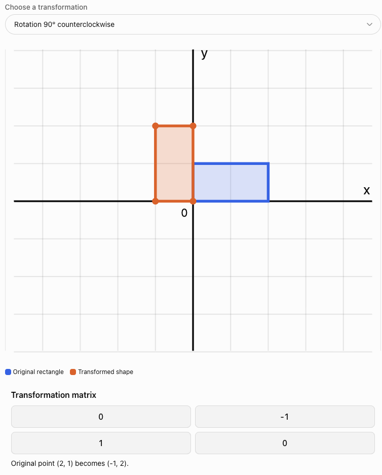
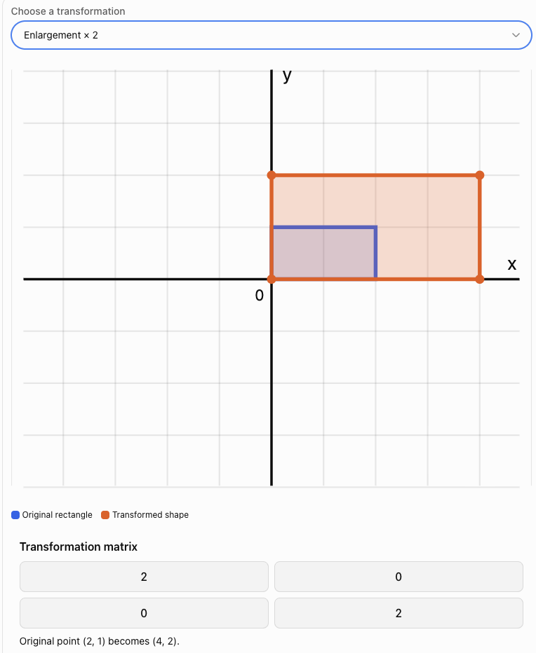
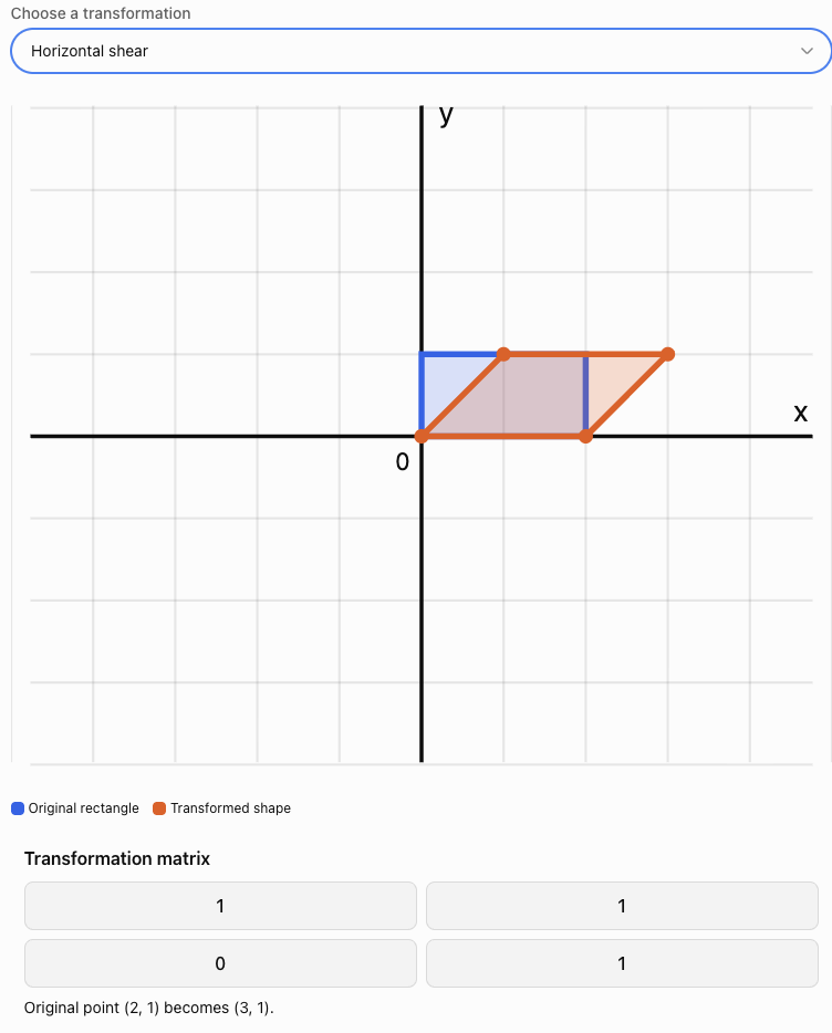
Rotation Matrices
A rotation turns an object through a specified angle around a fixed point.
For the standard 2 × 2 rotation matrix, the centre of rotation is the origin.
A positive angle represents a counterclockwise rotation.
A negative angle represents a clockwise rotation.
General rotation matrix
For a counterclockwise rotation through an angle θ:
The transformed coordinates are:
x′ = x cos θ − y sin θ
y′ = x sin θ + y cos θ
This formula works for any angle.
Rotation through 90° counterclockwise
Since:
cos 90° = 0
sin 90° = 1
the matrix becomes:
The coordinate rule is:
(x, y) → (−y, x)
Rotation through 180°
Since:
cos 180° = −1
sin 180° = 0
The coordinate rule is:
(x, y) → (−x, −y)
Rotation through 270° counterclockwise
The coordinate rule is:
(x, y) → (y, −x)
This is equivalent to a 90° clockwise rotation.
Summary of common rotation matrices
|
Rotation |
Matrix |
|---|---|
|
90° counterclockwise |
[[0, −1], [1, 0]] |
|
180° |
[[−1, 0], [0, −1]] |
|
270° counterclockwise |
[[0, 1], [−1, 0]] |
|
360° |
[[1, 0], [0, 1]] |
Worked Example 1: Rotation Through 90°
Rotate P(4, 2) through 90° counterclockwise about the origin.
Step 1: Write the rotation matrix.
Step 2: Write the position vector.
Step 3: Multiply.
x′ = 0(4) − 1(2) = −2
y′ = 1(4) + 0(2) = 4
Therefore:
Verification
The distance from the origin before rotation is:
√(4² + 2²) = √20
After rotation:
√((−2)² + 4²) = √20
The distance remains unchanged.
This is expected because rotations preserve distances.
Worked Example 2: Rotation Through 45°
Rotate P(2, 0) through 45° counterclockwise.
The rotation matrix is:
Multiply:
Therefore:
x′ = √2
y′ = √2
Approximately:
P′ ≈ (1.414, 1.414)
The point remains 2 units from the origin.
Reflection Matrices
A reflection produces a mirror image across a specified line.
Unlike rotations, reflections reverse orientation.
The shape and size remain unchanged.
Reflection in the x-axis
Coordinate rule:
(x, y) → (x, −y)
Reflection in the y-axis
Coordinate rule:
(x, y) → (−x, y)
Reflection in the line y = x
Coordinate rule:
(x, y) → (y, x)
Reflection in the line y = −x
Coordinate rule:
(x, y) → (−y, −x)
Worked Example 3: Reflection in the x-axis
Reflect P(3, 5) in the x-axis.
Therefore:
The x-coordinate remains unchanged, while the y-coordinate changes sign.
Worked Example 4: Reflection in the Line y = x
Reflect the point P(−2, 6) in the line y = x.
The matrix is:
Multiply:
Therefore:
The x- and y-coordinates exchange positions.
Enlargement Matrices
An enlargement changes the size of an object.
For an enlargement with scale factor k about the origin:
The coordinate rule is:
(x, y) → (kx, ky)
Interpreting the scale factor
-
k > 1: enlargement
-
0 < k < 1: reduction
-
k = 1: identity transformation
-
k = 0: collapse to the origin
-
k < 0: scaling combined with a 180° reversal in direction
Worked Example 5: Enlargement by Scale Factor 3
Enlarge P(2, −1) by scale factor 3 about the origin.
Therefore:
The distance from the origin becomes three times as large.
The area of any two-dimensional shape becomes 3² = 9 times as large.
Non-Uniform Stretches
A non-uniform stretch changes horizontal and vertical dimensions by different factors.
The general matrix is:
where:
-
a is the horizontal scale factor.
-
b is the vertical scale factor.
The coordinate rule is:
(x, y) → (ax, by)
Worked Example 6: Horizontal Stretch and Vertical Compression
A rectangle has vertices:
A(0, 0)
B(2, 0)
C(2, 4)
D(0, 4)
Apply:
This stretches horizontally by a factor of 3 and compresses vertically by a factor of 1/2.
The new vertices are:
A′(0, 0)
B′(6, 0)
C′(6, 2)
D′(0, 2)
Original area:
2 × 4 = 8 square units
Transformed area:
6 × 2 = 12 square units
Area scale factor:
12/8 = 1.5
This agrees with:
det(S) = 3(1/2) = 1.5
The determinant describes the signed area scale factor.
Shear Transformations
A shear changes the shape of an object by shifting points parallel to a particular axis.
A square may become a parallelogram.
Unlike an enlargement, a shear does not necessarily change the area.
Horizontal shear
The matrix is:
The coordinate rules are:
x′ = x + ky
y′ = y
Here, k is the shear factor.
A point moves horizontally by an amount proportional to its y-coordinate.
Vertical shear
The matrix is:
The coordinate rules are:
x′ = x
y′ = kx + y
A point moves vertically by an amount proportional to its x-coordinate.
Worked Example 7: Horizontal Shear
Apply the matrix:
to the point P(3, 2).
x′ = 3 + 2(2) = 7
y′ = 2
Therefore:
The point moves 4 units to the right.
Shearing a square
Consider the unit square with vertices:
(0, 0), (1, 0), (1, 1), (0, 1)
Apply a horizontal shear with k = 1.
The new vertices are:
(0, 0), (1, 0), (2, 1), (1, 1)
The square becomes a parallelogram.
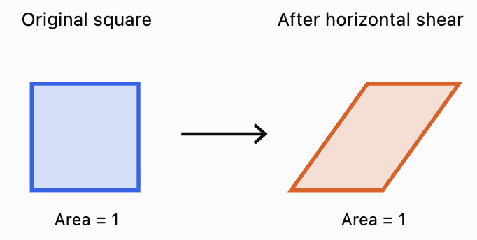
The shear changes the angles but preserves the area.
For a horizontal shear:
det(H) = 1(1) − k(0) = 1
Therefore, the area scale factor is 1.
Combining Transformations
One of the greatest advantages of matrix methods is that several transformations can be combined into a single matrix.
Suppose a point is first transformed by matrix A and then by matrix B.
The first transformation gives:
P′ = AP
The second gives:
P″ = BP′
Substitute:
P″ = B(AP)
Therefore:
The combined transformation matrix is BA, not AB.
The matrix closest to the original vector acts first.
Why order matters
Matrix multiplication is generally not commutative:
AB ≠ BA
Consequently, changing the order of geometric transformations may produce a different result.
Worked Example 8: Reflection Followed by Rotation
A point P(2, 3) is:
-
Reflected in the x-axis.
-
Rotated 90° counterclockwise about the origin.
Find its final coordinates.
Step 1: Write the reflection matrix.
Step 2: Write the rotation matrix.
Step 3: Construct the combined matrix.
Because the reflection happens first:
Combined matrix = RM
Multiplying:
Step 4: Apply the combined transformation.
Therefore:
Geometric interpretation
The combined matrix:
represents a reflection in the line y = x.
Therefore, reflecting in the x-axis and then rotating 90° counterclockwise is equivalent to reflecting in the line y = x.
Worked Example 9: Why Transformation Order Matters
Consider P(1, 2).
Let:
represent a 90° counterclockwise rotation.
Let:
represent a horizontal stretch by factor 2.
Case A: Stretch first, then rotate
The combined matrix is:
RS
Apply to P:
Final point:
(−2, 2)
Case B: Rotate first, then stretch
The combined matrix is:
SR
Apply to P:
Final point:
(−4, 1)
The results are different.
Therefore:
RS ≠ SR
The order of transformations is important.
Interpreting Transformation Matrices Geometrically
A transformation matrix contains information about how the coordinate axes are transformed.
Consider:
The first column:
shows where the unit vector (1, 0) is sent.
The second column:
shows where the unit vector (0, 1) is sent.
This gives a powerful method for understanding any 2 × 2 transformation.
Worked Example 10: Interpreting a Matrix
Consider:
Apply A to the unit vector e₁ = (1, 0):
Apply A to the unit vector e₂ = (0, 1):
Therefore:
-
The original horizontal unit vector becomes (2, 0).
-
The original vertical unit vector becomes (1, 3).
The unit square becomes a parallelogram with vertices:
(0, 0), (2, 0), (3, 3), (1, 3)
The transformation combines stretching and shearing.
The determinant and area
The determinant is:
det(A) = 2(3) − 1(0)
= 6
Therefore, areas are multiplied by 6.
A unit square with area 1 becomes a parallelogram with area 6.
Determinants and Geometric Transformations
The determinant of a 2 × 2 transformation matrix provides important geometric information.
For:
the determinant is:
det(A) = ad − bc
Geometric meaning
The absolute value of the determinant gives the area scale factor:
The sign of the determinant describes orientation.
|
Determinant |
Geometric meaning |
|---|---|
|
det(A) > 0 |
Orientation is preserved |
|
det(A) < 0 |
Orientation is reversed |
|
det(A) = 0 |
Area collapses to zero; transformation is singular |
|
det(A) = 1 |
Area and orientation are preserved |
|
det(A) = −1 |
Area is preserved but orientation is reversed |
Examples
Rotation matrix
det(R) = 1
Rotations preserve area and orientation.
Reflection matrix
det(M) = −1
Reflections preserve area but reverse orientation.
Enlargement by factor k
det(E) = k²
Areas are multiplied by k².
Horizontal shear
det(H) = 1
A shear preserves area and orientation.
Inverse Transformations
An inverse transformation reverses the effect of the original transformation.
If:
P′ = AP
then:
provided A is invertible.
Examples
-
The inverse of a 90° counterclockwise rotation is a 90° clockwise rotation.
-
The inverse of a reflection is the same reflection.
-
The inverse of an enlargement by factor 3 is an enlargement by factor 1/3.
-
The inverse of a horizontal shear with factor k is a horizontal shear with factor −k.
Worked Example 11: Reversing a Shear
A point is transformed using:
The transformed point is P′(9, 3).
Find the original point.
Step 1: Find the inverse.
Since det(H) = 1:
Step 2: Apply the inverse.
Therefore:
Transformations About Points Other Than the Origin
Ordinary 2 × 2 matrices describe linear transformations that leave the origin fixed.
However, we may want to rotate or enlarge a shape about another point.
For example, suppose we want to rotate P(x, y) through an angle θ about C(h, k).
We can perform three steps:
-
Translate the centre C to the origin.
-
Apply the rotation.
-
Translate back.
The formula is:
Worked Example 12: Rotation About Another Point
Rotate P(5, 3) through 90° counterclockwise about C(2, 1).
Step 1: Subtract the centre.
P − C = (5 − 2, 3 − 1)
= (3, 2)
Step 2: Rotate through 90°.
(3, 2) → (−2, 3)
Step 3: Add the centre back.
P′ = (−2 + 2, 3 + 1)
Therefore:
Homogeneous coordinates
Translations can also be represented using matrices by introducing a third coordinate.
The point (x, y) becomes:
A translation by (h, k) is represented by:
This method is called homogeneous coordinates.
It is widely used in computer graphics because rotations, translations, stretches, and other affine transformations can then be combined through matrix multiplication.
Real-World Applications
Computer Graphics and Animation
Computer graphics systems use matrices to move, rotate, resize, and distort objects.
A video game character may be represented by thousands of vertices.
Instead of transforming each vertex using separate geometric constructions, the computer applies transformation matrices.
A character can be:
-
Rotated to face a new direction.
-
Enlarged or reduced.
-
Reflected to create a mirrored appearance.
-
Sheared to produce visual effects.
-
Moved through a scene using homogeneous transformation matrices.
Multiple transformations can be combined into one matrix, improving computational efficiency.
Robotics
Robotic arms contain joints that rotate and move.
Matrices describe how the position of one joint relates to another.
By combining transformation matrices, engineers can calculate the position and orientation of a robot's end effector.
This is important for:
-
Manufacturing
-
Surgical robotics
-
Automated warehouses
-
Space exploration
-
Precision engineering
Architecture and Engineering
Architects use geometric transformations when creating and modifying designs.
A structural component may need to be rotated, reflected, or scaled.
Shear transformations are also important in understanding how shapes deform under certain loads.
Image Processing
Digital images can be transformed using matrices.
Examples include:
-
Rotating photographs
-
Reflecting images
-
Resizing images
-
Correcting perspective
-
Creating visual effects
In practical image processing, transformed pixel positions are calculated and image values are resampled to produce the final image.
Common Mistakes
Mistake 1: Multiplying matrices in the wrong order
If A happens first and B second, the combined matrix is BA.
Mistake 2: Confusing clockwise and counterclockwise rotation
A positive angle in the standard rotation matrix means counterclockwise.
Mistake 3: Using row vectors instead of column vectors without adjusting the convention
The matrices in this lesson assume column vectors.
Mistake 4: Forgetting that standard 2 × 2 transformations are about the origin
Transformations about other points require translations or homogeneous coordinates.
Mistake 5: Confusing reflections in the x-axis and y-axis
Reflection in the x-axis changes the sign of y. Reflection in the y-axis changes the sign of x.
Mistake 6: Assuming every transformation preserves area
Rotations, reflections, and standard shears preserve area. Enlargements and non-uniform stretches may change area.
Mistake 7: Confusing scale factor with area scale factor
An enlargement by factor k changes area by k².
Mistake 8: Assuming matrix multiplication is commutative
In general, AB ≠ BA.
Mistake 9: Ignoring the determinant
The determinant gives useful information about area, orientation, and invertibility.
Mistake 10: Assuming every matrix represents a pure rotation or reflection
Some matrices combine several geometric effects.
Mistake 11: Rounding trigonometric values too early
Keep exact values where possible to avoid unnecessary errors.
Mistake 12: Forgetting to transform every vertex
To transform a polygon, apply the matrix to all its vertices.
Key Terms
-
Geometric Transformation: Change in the position, orientation, size, or shape of an object.
-
Transformation Matrix: Matrix representing a geometric transformation.
-
Position Vector: Vector representing a point relative to the origin.
-
Image: Result of applying a transformation to a point or shape.
-
Preimage: Original point or shape before transformation.
-
Rotation: Transformation turning an object through an angle.
-
Centre of Rotation: Fixed point around which a rotation occurs.
-
Reflection: Transformation producing a mirror image.
-
Line of Reflection: Line acting as the mirror.
-
Enlargement: Transformation changing an object's size by a scale factor.
-
Scale Factor: Number describing how lengths change.
-
Uniform Scaling: Scaling equally in every direction.
-
Non-Uniform Stretch: Scaling by different factors in different directions.
-
Compression: Transformation reducing lengths in a particular direction.
-
Shear: Transformation shifting points parallel to an axis by an amount dependent on position.
-
Horizontal Shear: Shear that changes x-coordinates.
-
Vertical Shear: Shear that changes y-coordinates.
-
Composite Transformation: Combination of two or more transformations.
-
Identity Matrix: Matrix representing no change.
-
Inverse Transformation: Transformation reversing an original transformation.
-
Determinant: Scalar describing area scaling, orientation, and invertibility.
-
Orientation: Directional ordering of points in a shape.
-
Area Scale Factor: Factor by which areas change.
-
Singular Matrix: Matrix with determinant zero.
-
Unit Vector: Vector of length one.
-
Linear Transformation: Transformation preserving vector addition and scalar multiplication.
-
Affine Transformation: Transformation combining a linear transformation and translation.
-
Homogeneous Coordinates: Coordinate system allowing translations to be represented using matrices.
-
Translation: Transformation shifting every point by the same displacement.
-
Invariant Point: Point unchanged by a transformation.
Key Takeaways
-
Geometric transformations can be represented using matrices.
-
A point P is transformed using P′ = AP.
-
Rotation matrices use sine and cosine functions.
-
A positive rotation angle represents counterclockwise rotation.
-
Reflections reverse orientation but preserve distances and area.
-
Enlargements change lengths according to a scale factor.
-
A uniform enlargement by factor k changes areas by k².
-
Non-uniform stretches scale horizontal and vertical dimensions differently.
-
Shears change shape while preserving area.
-
Composite transformations are calculated using matrix multiplication.
-
The order of transformations matters.
-
The columns of a transformation matrix show where the coordinate unit vectors are sent.
-
The absolute determinant gives the area scale factor.
-
A negative determinant indicates reversed orientation.
-
An inverse matrix reverses an invertible transformation.
-
Transformations about other centres can be handled using translations.
-
Homogeneous coordinates allow affine transformations to be combined using matrices.
-
Matrix transformations are important in computer graphics, engineering, robotics, and image processing.
Check Your Understanding
Questions
Question 1: Rotation
Rotate P(3, 4) through 90° counterclockwise about the origin.
Question 2: Rotation Through 180°
Rotate P(−5, 2) through 180° about the origin.
Question 3: Reflection in the x-axis
Reflect P(4, −7) in the x-axis.
Question 4: Reflection in y = x
Reflect P(−3, 6) in the line y = x.
Question 5: Enlargement
Enlarge P(2, −4) by scale factor 3 about the origin.
Question 6: Non-Uniform Stretch
Apply:
to P(3, 8).
Question 7: Horizontal Shear
Apply:
to P(2, 4).
Question 8: Vertical Shear
Apply:
to P(3, 1).
Question 9: Combined Transformations
A point is reflected in the x-axis and then rotated through 90° counterclockwise.
Find the combined transformation matrix.
Question 10: Transformation Order
Explain why the order of transformations matters.
Question 11: Determinant and Area
A transformation matrix is:
Determine the area scale factor.
Question 12: Orientation
Determine whether:
preserves or reverses orientation.
Question 13: Inverse Transformation
Find the inverse of:
Question 14: Rotation About Another Point
Rotate P(6, 4) through 90° counterclockwise about C(2, 2).
Question 15: Integrated Challenge
A triangle has vertices:
A(1, 1)
B(3, 1)
C(2, 4)
The triangle is first enlarged by scale factor 2 about the origin and then reflected in the y-axis.
a) Write the enlargement matrix.
b) Write the reflection matrix.
c) Find the combined transformation matrix.
d) Calculate the transformed vertices.
e) Calculate the original and transformed areas.
f) Explain the geometric meaning of the determinant.
Fully Worked Answers
Answer 1: Rotation
A 90° counterclockwise rotation uses:
Answer: (−4, 3)
Answer 2: Rotation Through 180°
A 180° rotation changes the signs of both coordinates.
(−5, 2) → (5, −2)
Answer: (5, −2)
Answer 3: Reflection in the x-axis
The x-coordinate stays the same.
The y-coordinate changes sign.
(4, −7) → (4, 7)
Answer: (4, 7)
Answer 4: Reflection in y = x
The coordinates exchange positions.
(−3, 6) → (6, −3)
Answer: (6, −3)
Answer 5: Enlargement
Scale factor = 3
Multiply both coordinates by 3.
(2, −4) → (6, −12)
Answer: (6, −12)
Answer 6: Non-Uniform Stretch
x′ = 2(3) = 6
y′ = (1/2)(8) = 4
Answer: (6, 4)
Answer 7: Horizontal Shear
x′ = 2 + 3(4) = 14
y′ = 4
Answer: (14, 4)
Answer 8: Vertical Shear
x′ = 3
y′ = 2(3) + 1 = 7
Answer: (3, 7)
Answer 9: Combined Transformations
Reflection in x-axis:
Rotation 90° counterclockwise:
Reflection happens first, so:
Combined matrix = RM
This is equivalent to reflection in y = x.
Answer 10: Transformation Order
Matrix multiplication is generally not commutative.
Therefore:
AB ≠ BA
Applying A first and then B gives BA.
Applying B first and then A gives AB.
These may produce different transformed coordinates.
Answer: The order matters because different transformation sequences can produce different final positions and shapes.
Answer 11: Determinant and Area
det(A) = 3(2) − 1(0)
= 6
Area scale factor = |6|
Answer: 6
Areas become six times as large.
Answer 12: Orientation
det(A) = −1(1) − 0
= −1
The determinant is negative.
Answer: Orientation is reversed.
The transformation is a reflection in the y-axis.
Answer 13: Inverse Transformation
The inverse reverses the stretches.
Answer 14: Rotation About Another Point
Point:
P(6, 4)
Centre:
C(2, 2)
Subtract the centre:
P − C = (4, 2)
Rotate 90° counterclockwise:
(4, 2) → (−2, 4)
Add the centre back:
(−2 + 2, 4 + 2)
Answer: (0, 6)
Answer 15: Integrated Challenge
Original vertices:
A(1, 1)
B(3, 1)
C(2, 4)
Part a: Enlargement matrix
Scale factor = 2
Part b: Reflection matrix
Reflection in the y-axis:
Part c: Combined matrix
Enlargement happens first, then reflection.
Therefore:
Combined matrix = ME
Part d: Transformed vertices
Apply:
(x, y) → (−2x, 2y)
A(1, 1) → A′(−2, 2)
B(3, 1) → B′(−6, 2)
C(2, 4) → C′(−4, 8)
Therefore:
A′(−2, 2), B′(−6, 2), C′(−4, 8)
Part e: Areas
Original triangle:
Base = 3 − 1 = 2
Height = 4 − 1 = 3
Area = 1/2 × 2 × 3
= 3 square units
Transformed triangle:
Base = |−6 − (−2)| = 4
Height = 8 − 2 = 6
Area = 1/2 × 4 × 6
= 12 square units
Area scale factor:
12/3 = 4
Part f: Determinant
The combined matrix is:
det(A) = (−2)(2) − 0
= −4
The absolute determinant is 4, so areas are multiplied by 4.
The negative sign indicates that orientation is reversed.
This agrees with the transformation: enlargement changes area by factor 4, while reflection reverses orientation.
Final Reflection
Matrices provide an efficient and systematic way to describe geometric transformations.
Rotations and reflections change the orientation or position of shapes while preserving their size. Enlargements and stretches change dimensions, while shears alter shape by shifting points in a particular direction.
Combining transformations through matrix multiplication allows complicated geometric operations to be represented by a single matrix.
The order of multiplication is essential because transformations generally do not commute.
The determinant provides a further connection between algebra and geometry, describing area scaling, orientation, and whether a transformation can be reversed.
These ideas form an important foundation for computer graphics, robotics, engineering, and advanced geometry.
The central idea is that a transformation matrix encodes a geometric rule, allowing points and entire shapes to be transformed, combined, analysed, and reversed using matrix operations.
2. Eigenvalues and Eigenvectors
Learning outcomes
- I can define eigenvalues and eigenvectors.
- I can calculate simple eigenvalues.
- I can determine corresponding eigenvectors.
- I can interpret their geometric meaning.
- I can recognise applications of eigenvalues.
Introduction
When a matrix transforms a vector, it usually changes both the vector's length and its direction. However, some vectors behave differently: after the transformation, they remain on the same line through the origin.
These special vectors are called eigenvectors, and the numbers describing how they are scaled are called eigenvalues.
Eigenvalues and eigenvectors are important because they reveal the underlying behaviour of matrix transformations. They help mathematicians and scientists understand how systems change, which directions remain unchanged, and whether processes grow, shrink, or remain stable.
They are used in many areas, including:
-
Physics: vibrations, forces, and quantum mechanics.
-
Engineering: structural stability and mechanical systems.
-
Computer science: image processing and machine learning.
-
Biology: population growth and ecological models.
-
Economics: long-term behaviour of economic systems.
-
Data science: principal component analysis and dimensionality reduction.
In this lesson, we will investigate how to identify, calculate, and interpret eigenvalues and eigenvectors, beginning with simple 2 × 2 matrices and progressing to practical applications.
What Are Eigenvalues and Eigenvectors?
Consider a square matrix A acting on a nonzero vector v.
Normally, multiplying A by v changes the direction and magnitude of v.
However, for certain vectors, the result is simply a scalar multiple of the original vector.
This relationship is written as:
where:
-
A is a square matrix representing a linear transformation.
-
v is a nonzero eigenvector.
-
λ (lambda) is the corresponding eigenvalue.
-
Av is the transformed vector.
An eigenvector is a nonzero vector whose direction stays on the same line after the transformation.
An eigenvalue is the scalar by which that eigenvector is multiplied.
Interpreting the eigenvalue
|
Eigenvalue |
Geometric meaning |
|---|---|
|
λ > 1 |
Vector becomes longer, same direction |
|
λ = 1 |
Vector remains unchanged |
|
0 < λ < 1 |
Vector becomes shorter, same direction |
|
λ = 0 |
Vector collapses to the zero vector |
|
−1 < λ < 0 |
Vector becomes shorter and reverses direction |
|
λ = −1 |
Vector reverses direction, same length |
|
λ < −1 |
Vector becomes longer and reverses direction |
The eigenvector must be nonzero. Otherwise, every matrix would trivially satisfy A0 = λ0 for any λ.
A Geometric Illustration
Consider the transformation:
This stretches the x-direction by a factor of 2 and compresses the y-direction by a factor of 1/2.
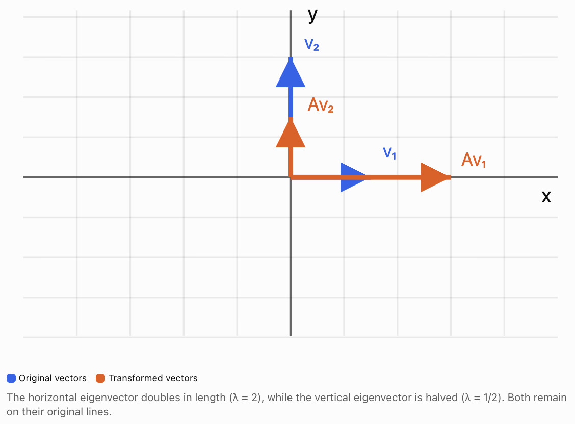
The x-axis and y-axis are special directions for this transformation.
Any nonzero vector along the x-axis is an eigenvector with eigenvalue 2.
Any nonzero vector along the y-axis is an eigenvector with eigenvalue 1/2.
Vectors that do not lie along these axes generally change direction.
Identifying Eigenvalues from Simple Matrices
Some matrices have eigenvalues that can be recognised immediately.
Diagonal matrices
Consider:
The matrix multiplies horizontal components by 4 and vertical components by 3.
Therefore:
-
λ₁ = 4, corresponding to horizontal eigenvectors.
-
λ₂ = 3, corresponding to vertical eigenvectors.
For a diagonal matrix, the diagonal entries are its eigenvalues.
Identity matrix
For every vector v:
Iv = v
Therefore, every nonzero vector is an eigenvector with eigenvalue 1.
Zero matrix
For every vector v:
Ov = 0v
Therefore, every nonzero vector is an eigenvector with eigenvalue 0.
Calculating Eigenvalues
For a general matrix, eigenvalues can be found using the characteristic equation.
Start with:
Since I is the identity matrix:
Rearrange:
For a nonzero solution v to exist, the matrix A − λI must be singular.
Therefore:
This is called the characteristic equation.
The expression det(A − λI) is the characteristic polynomial.
Its roots are the eigenvalues.
General formula for a 2 × 2 matrix
Let:
Then:
Calculate the determinant:
Expand:
ad − aλ − dλ + λ² − bc = 0
Rearrange:
Since a + d is the trace of A and ad − bc is its determinant:
This provides a useful connection between eigenvalues, trace, and determinant.
Worked Example 1: Calculating Eigenvalues
Find the eigenvalues of:
Step 1: Construct A − λI.
Step 2: Calculate the determinant.
Expand:
9 − 6λ + λ² − 1 = 0
Therefore:
λ² − 6λ + 8 = 0
Step 3: Factorise.
(λ − 2)(λ − 4) = 0
Therefore:
These are the eigenvalues of A.
Verification using trace and determinant
Trace:
tr(A) = 3 + 3 = 6
Sum of eigenvalues:
2 + 4 = 6
Determinant:
det(A) = 3(3) − 1(1) = 8
Product of eigenvalues:
2 × 4 = 8
Both relationships are satisfied.
Calculating Eigenvectors
After finding an eigenvalue, we determine its corresponding eigenvectors.
We use:
For a 2 × 2 matrix, write:
Substitute the eigenvalue and solve the resulting homogeneous system.
Eigenvectors are not unique.
If v is an eigenvector, then any nonzero scalar multiple kv is also an eigenvector corresponding to the same eigenvalue.
The set of all eigenvectors associated with an eigenvalue, together with the zero vector, forms an eigenspace.
Worked Example 2: Finding Corresponding Eigenvectors
Continue with:
We found:
λ₁ = 2
λ₂ = 4
Eigenvector for λ = 2
Substitute into:
(A − 2I)v = 0
This gives:
x + y = 0
Therefore:
y = −x
Choose x = 1.
Then y = −1.
An eigenvector is:
Any nonzero multiple of this vector is also valid.
Eigenvector for λ = 4
Substitute into:
(A − 4I)v = 0
This gives:
−x + y = 0
Therefore:
y = x
Choose x = 1.
Then y = 1.
An eigenvector is:
Verification
For v₁:
For v₂:
Both eigenvectors are correct.
Geometric Meaning of Eigenvectors
Eigenvectors identify directions that are preserved by a linear transformation, although the vector may reverse direction or become zero.
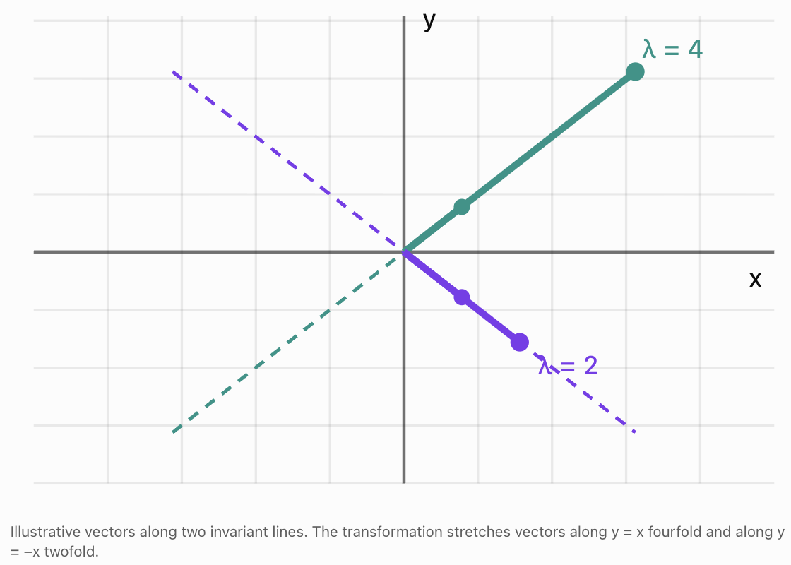
Consider again:
Its eigenvectors lie along:
y = x
and:
y = −x
Along y = x, the matrix stretches vectors by factor 4.
Along y = −x, it stretches vectors by factor 2.
Why this is important
A complicated transformation may behave simply along its eigenvector directions.
If we can identify those directions, we can understand the transformation more easily.
This becomes especially useful when the same matrix is applied repeatedly.
Worked Example 3: A Matrix with a Negative Eigenvalue
Consider:
The eigenvalues are:
λ₁ = −2
λ₂ = 3
For λ₁ = −2, an eigenvector is:
Apply the matrix:
The vector doubles in length and reverses direction.
For λ₂ = 3:
Apply the matrix:
The vector triples in length without reversing direction.
A negative eigenvalue therefore indicates reversal along the corresponding eigenvector line.
Repeated Matrix Transformations
Eigenvalues are particularly useful when the same transformation is applied repeatedly.
Suppose:
Apply A again:
Since λ is a scalar:
Therefore:
Repeating this process gives:
This means we can predict the effect of repeated transformations on eigenvectors without calculating large matrix powers.
Worked Example 4: Repeated Transformations
Suppose:
Find A⁴v.
Using the eigenvalue relationship:
A⁴v = 3⁴v
Therefore:
After four applications, the vector is 81 times its original length, with the same direction.
Growth and decay
If |λ| > 1, repeated transformations increase the vector's magnitude.
If 0 < |λ| < 1, repeated transformations decrease its magnitude.
If |λ| = 1, the magnitude remains unchanged.
If λ = 0, the vector becomes zero after one transformation.
Negative eigenvalues cause the direction to alternate with successive transformations.
Eigenvalues and Matrix Properties
Eigenvalues are connected to several important properties of matrices.
Trace and eigenvalues
For a 2 × 2 matrix:
the trace is:
tr(A) = a + d
The sum of the eigenvalues, counting multiplicity, is:
Determinant and eigenvalues
The product of the eigenvalues is:
Worked Example 5: Using Trace and Determinant
A 2 × 2 matrix has:
tr(A) = 9
det(A) = 20
Find its eigenvalues.
We know:
λ₁ + λ₂ = 9
λ₁λ₂ = 20
The characteristic equation is:
λ² − 9λ + 20 = 0
Factorise:
(λ − 4)(λ − 5) = 0
Therefore:
This method avoids calculating the characteristic determinant from scratch.
Eigenvalues and Singular Matrices
A square matrix is singular if its determinant is zero.
Since the determinant equals the product of the eigenvalues:
for a 2 × 2 matrix, if either eigenvalue is zero:
det(A) = 0
Therefore, the matrix is singular.
Worked Example 6: A Zero Eigenvalue
Consider:
Calculate the determinant:
det(A) = 2(2) − 4(1)
= 0
The matrix is singular.
Its characteristic equation is:
λ² − 4λ = 0
Factorise:
λ(λ − 4) = 0
Therefore:
The zero eigenvalue indicates that some nonzero vectors are transformed into the zero vector.
For example:
Then:
This confirms that v is an eigenvector with eigenvalue zero.
Matrices with Repeated Eigenvalues
A matrix may have the same eigenvalue more than once.
Consider:
Its characteristic equation is:
(3 − λ)² = 0
Therefore:
λ = 3 is a repeated eigenvalue.
Every nonzero vector is an eigenvector because:
Av = 3v
However, repeated eigenvalues do not always mean every vector is an eigenvector.
For example:
also has eigenvalue 3 repeated twice.
But:
The eigenvector equation gives:
y = 0
Therefore, its eigenvectors are only the nonzero vectors along the x-axis.
This distinction becomes important when studying diagonalisation.
Eigenvalues and Diagonalisation
Some matrices can be rewritten in a simpler form using their eigenvectors.
If a 2 × 2 matrix has two linearly independent eigenvectors, we can form a matrix P using those eigenvectors as columns.
The matrix can then be expressed as:
where D is a diagonal matrix containing the corresponding eigenvalues.
For example, if:
λ₁ = 2
λ₂ = 5
then:
Diagonalisation is useful because powers of diagonal matrices are easy to calculate:
Therefore:
This provides an efficient method for studying repeated transformations and long-term behaviour.
Not every matrix is diagonalizable, but many important matrices are.
Complex Eigenvalues
Not every real matrix has real eigenvalues.
Consider a rotation through 90° counterclockwise:
Its characteristic equation is:
λ² + 1 = 0
Therefore:
λ² = −1
The eigenvalues are:
where i² = −1.
This explains why a 90° rotation has no nonzero real eigenvectors: every nonzero real vector changes direction.
Complex eigenvalues are important in advanced mathematics, oscillations, electrical engineering, and dynamical systems.
Real-World Application 1: Population Growth
Eigenvalues can be used to predict how populations change over time.
Consider a simplified population divided into two age groups:
-
Juveniles
-
Adults
Suppose the population changes each year according to:
The matrix describes reproduction and survival.
Its characteristic equation is:
Therefore:
−λ(0.5 − λ) − 1 = 0
λ² − 0.5λ − 1 = 0
Using the quadratic formula:
Approximately:
λ₁ ≈ 1.281
λ₂ ≈ −0.781
The dominant eigenvalue is approximately 1.281.
In this simplified model, the long-term population grows by approximately 28.1% per year, provided the model remains valid and the initial population has a positive contribution along the dominant eigenvector.
The corresponding eigenvector describes the stable proportion of juveniles and adults approached over time.
Why this matters
Population models can help scientists investigate:
-
Species conservation
-
Wildlife management
-
Fisheries
-
Age distributions
-
Long-term population trends
The results depend on the assumptions and accuracy of the model.
Real-World Application 2: Mechanical Vibrations
Engineers study how buildings, bridges, vehicles, and machines vibrate.
A mechanical system may have several possible vibration patterns.
Each natural vibration pattern is called a mode shape.
Eigenvectors describe these mode shapes, while eigenvalues are related to the corresponding natural frequencies.
For a simple undamped system:
where:
-
K is the stiffness matrix.
-
M is the mass matrix.
-
v is a mode shape.
-
ω is the angular frequency.
This is a generalised eigenvalue problem.
Engineers use these calculations to help prevent dangerous resonance and improve structural designs.
Real-World Application 3: Data Science and Principal Component Analysis
Principal component analysis (PCA) is a technique used to identify important patterns in data.
Suppose a dataset contains two related variables, such as height and arm span.
The data points may form an elongated cloud.
A covariance matrix describes how the variables vary together.
The eigenvectors of this matrix identify the principal directions of variation.
The corresponding eigenvalues describe how much variance lies along those directions.
The eigenvector with the largest eigenvalue identifies the direction of greatest variation.
This is useful for:
-
Reducing the number of variables in datasets.
-
Visualising high-dimensional data.
-
Identifying patterns.
-
Compressing information.
-
Preparing data for machine learning.
Real-World Application 4: Search Engines and Networks
Large networks can be represented using matrices.
For example, a network may represent:
-
Webpages and hyperlinks.
-
People and social connections.
-
Transport routes.
-
Communication systems.
Eigenvectors can help identify important or influential nodes in a network.
In eigenvector centrality, a node is considered important when it is connected to other important nodes.
Related ideas are used in ranking algorithms and network analysis.
Common Mistakes
Mistake 1: Confusing eigenvalues with eigenvectors
An eigenvalue is a scalar. An eigenvector is a nonzero vector.
Mistake 2: Forgetting that eigenvectors must be nonzero
The zero vector is not an eigenvector.
Mistake 3: Calculating det(A) instead of det(A − λI)
The characteristic equation requires subtracting λ from the diagonal entries.
Mistake 4: Making sign errors in determinants
For a 2 × 2 matrix, the determinant is ad − bc.
Mistake 5: Finding eigenvalues but not eigenvectors
Each eigenvalue must be substituted into (A − λI)v = 0 to find corresponding eigenvectors.
Mistake 6: Assuming eigenvectors are unique
Any nonzero scalar multiple of an eigenvector is also an eigenvector.
Mistake 7: Assuming all matrices have real eigenvalues
Some real matrices have complex eigenvalues.
Mistake 8: Assuming every vector is an eigenvector
Only vectors satisfying Av = λv for some scalar λ are eigenvectors.
Mistake 9: Misinterpreting negative eigenvalues
A negative eigenvalue reverses direction along the eigenvector line.
Mistake 10: Assuming repeated eigenvalues always provide multiple independent eigenvectors
Some matrices have repeated eigenvalues but only one independent eigenvector.
Mistake 11: Forgetting to verify eigenvectors
Always check Av = λv.
Mistake 12: Confusing eigenvalue magnitude with vector length
The eigenvalue is a scaling factor, not necessarily the length of the eigenvector.
Key Terms
-
Eigenvalue: Scalar describing how an eigenvector is scaled by a matrix.
-
Eigenvector: Nonzero vector transformed into a scalar multiple of itself.
-
Linear Transformation: Transformation preserving vector addition and scalar multiplication.
-
Characteristic Equation: Equation det(A − λI) = 0 used to find eigenvalues.
-
Characteristic Polynomial: Polynomial obtained from det(A − λI).
-
Identity Matrix: Matrix that leaves vectors unchanged when multiplied.
-
Determinant: Scalar associated with a square matrix, indicating invertibility and geometric scaling.
-
Trace: Sum of the diagonal entries of a square matrix.
-
Eigenspace: Set of eigenvectors associated with an eigenvalue, together with the zero vector.
-
Scalar Multiple: Vector obtained by multiplying another vector by a number.
-
Singular Matrix: Square matrix with determinant zero.
-
Non-Singular Matrix: Square matrix with a nonzero determinant.
-
Repeated Eigenvalue: Eigenvalue appearing more than once as a root of the characteristic polynomial.
-
Diagonal Matrix: Matrix with zeros outside its main diagonal.
-
Diagonalisation: Process of expressing a matrix as PDP⁻¹.
-
Dominant Eigenvalue: Eigenvalue with the greatest absolute value, when one is strictly greatest.
-
Matrix Power: Repeated multiplication of a matrix by itself.
-
Stable Distribution: Long-term relative distribution approached in certain population models.
-
Principal Component Analysis: Data analysis technique using eigenvectors and eigenvalues of a covariance matrix.
-
Covariance Matrix: Matrix describing variances and covariances between variables.
-
Mode Shape: Natural pattern of vibration in a mechanical system.
-
Natural Frequency: Frequency at which a system naturally oscillates.
-
Complex Eigenvalue: Eigenvalue containing an imaginary component.
-
Invariant Direction: Direction preserved by a linear transformation.
-
Dynamical System: System describing how quantities change over time.
Key Takeaways
-
Eigenvectors are nonzero vectors that remain on the same line after a matrix transformation.
-
Eigenvalues describe the scaling of corresponding eigenvectors.
-
The defining equation is Av = λv.
-
Eigenvalues are found using det(A − λI) = 0.
-
Eigenvectors are found by solving (A − λI)v = 0.
-
A matrix may have several eigenvalues and corresponding eigenspaces.
-
Any nonzero scalar multiple of an eigenvector is also an eigenvector.
-
Positive eigenvalues preserve direction along an eigenvector.
-
Negative eigenvalues reverse direction.
-
Zero eigenvalues indicate that some nonzero vectors collapse to zero.
-
The sum of eigenvalues equals the trace, counting multiplicity.
-
The product of eigenvalues equals the determinant, counting multiplicity.
-
Repeated transformations satisfy Aⁿv = λⁿv.
-
Eigenvalues help explain growth, decay, and long-term behaviour.
-
Eigenvectors reveal important directions in geometric transformations.
-
Eigenvalues and eigenvectors are widely used in physics, engineering, biology, economics, and data science.
Check Your Understanding
Questions
Question 1: Definition
Explain the difference between an eigenvalue and an eigenvector.
Question 2: Recognising Eigenvalues
Find the eigenvalues of:
Question 3: Checking an Eigenvector
Determine whether:
is an eigenvector of:
If so, find the eigenvalue.
Question 4: Characteristic Equation
Write the characteristic equation for:
Question 5: Calculating Eigenvalues
Find the eigenvalues of:
Question 6: Calculating Eigenvectors
Find eigenvectors corresponding to the eigenvalues in Question 5.
Question 7: Geometric Meaning
Explain what an eigenvalue of −3 means geometrically.
Question 8: Repeated Transformations
If Av = 2v, calculate A⁵v.
Question 9: Trace and Determinant
A 2 × 2 matrix has eigenvalues 3 and 7.
Find its trace and determinant.
Question 10: Singular Matrices
Explain why a matrix with eigenvalue zero must be singular.
Question 11: Repeated Eigenvalues
Find the eigenvalues of:
Describe its eigenvectors.
Question 12: Rotation Matrix
Explain why a 90° rotation matrix has no nonzero real eigenvectors.
Question 13: Growth Model
A population model has dominant eigenvalue 1.05.
Interpret this value.
Question 14: Data Science
Explain how eigenvectors and eigenvalues are used in principal component analysis.
Question 15: Integrated Challenge
Consider:
a) Calculate the characteristic polynomial.
b) Find the eigenvalues.
c) Find an eigenvector for each eigenvalue.
d) Verify both eigenvectors.
e) Calculate the trace and determinant.
f) Explain the geometric meaning of the transformation.
Fully Worked Answers
Answer 1: Definition
An eigenvector is a nonzero vector that is transformed into a scalar multiple of itself.
An eigenvalue is the scalar multiplying that eigenvector.
They satisfy:
Av = λv
For example, if Av = 4v, then v is an eigenvector and 4 is its eigenvalue.
Answer 2: Recognising Eigenvalues
This is a diagonal matrix.
Its eigenvalues are its diagonal entries.
Answer 3: Checking an Eigenvector
Multiply:
This equals:
Therefore:
Yes, v is an eigenvector with eigenvalue 4.
Answer 4: Characteristic Equation
Calculate:
(2 − λ)² − 1 = 0
Expand:
4 − 4λ + λ² − 1 = 0
Therefore:
Answer 5: Calculating Eigenvalues
Characteristic equation:
Expand:
12 − 7λ + λ² − 2 = 0
Therefore:
λ² − 7λ + 10 = 0
Factorise:
(λ − 5)(λ − 2) = 0
Answer 6: Calculating Eigenvectors
For λ = 5:
The eigenvector equation gives:
−x + y = 0
Therefore:
y = x
Choose:
For λ = 2:
The equation gives:
2x + y = 0
Therefore:
y = −2x
Choose:
Answer 7: Geometric Meaning
An eigenvalue of −3 means:
-
The eigenvector becomes three times as long.
-
Its direction is reversed.
-
It remains on the same line through the origin.
Answer 8: Repeated Transformations
Given:
Av = 2v
Then:
A⁵v = 2⁵v
Therefore:
Answer 9: Trace and Determinant
Eigenvalues:
3 and 7
Trace:
3 + 7 = 10
Determinant:
3 × 7 = 21
Answer: Trace = 10, determinant = 21.
Answer 10: Singular Matrices
The determinant of a square matrix equals the product of its eigenvalues, counting multiplicity.
If one eigenvalue is zero, the product is zero.
Therefore:
det(A) = 0
A matrix with determinant zero is singular.
Answer 11: Repeated Eigenvalues
The characteristic equation is:
(6 − λ)² = 0
Therefore:
λ = 6 is repeated twice.
Since A = 6I:
Av = 6v
for every vector v.
Answer: Every nonzero vector is an eigenvector with eigenvalue 6.
Answer 12: Rotation Matrix
A 90° rotation changes the direction of every nonzero real vector.
Therefore, no nonzero real vector remains on its original line.
Consequently, the matrix has no real eigenvectors.
Its eigenvalues are complex:
λ = i and λ = −i.
Answer 13: Growth Model
A dominant eigenvalue of 1.05 indicates that the dominant long-term population growth factor is approximately 1.05 per time period.
This corresponds to approximately 5% growth per period.
The interpretation assumes the model remains valid and the dominant eigenvalue controls the long-term population behaviour.
Answer 14: Data Science
In principal component analysis:
-
Eigenvectors of the covariance matrix identify directions of variation.
-
Eigenvalues describe the amount of variance along those directions.
-
The eigenvector with the largest eigenvalue identifies the direction of greatest variance.
PCA can reduce the number of variables while preserving much of the important information.
Answer 15: Integrated Challenge
Given:
Part a: Characteristic polynomial
Calculate:
(2 − λ)² − 1
= λ² − 4λ + 3
Therefore:
Part b: Eigenvalues
Solve:
λ² − 4λ + 3 = 0
Factorise:
(λ − 1)(λ − 3) = 0
Therefore:
Part c: Eigenvectors
For λ = 1:
Therefore:
x + y = 0
Choose:
For λ = 3:
Therefore:
y = x
Choose:
Part d: Verification
For λ = 1:
Therefore:
Av₁ = 1v₁
For λ = 3:
Therefore:
Av₂ = 3v₂
Both eigenvectors are correct.
Part e: Trace and determinant
Trace:
tr(A) = 2 + 2 = 4
Sum of eigenvalues:
1 + 3 = 4
Determinant:
det(A) = 2(2) − 1(1) = 3
Product of eigenvalues:
1 × 3 = 3
Both relationships are satisfied.
Part f: Geometric meaning
The eigenvector (1, −1) lies along y = −x.
Its eigenvalue is 1, so vectors along this direction remain unchanged.
The eigenvector (1, 1) lies along y = x.
Its eigenvalue is 3, so vectors along this direction are stretched by factor 3.
Therefore, the transformation stretches space along y = x while leaving vectors along y = −x unchanged.
The area scale factor is:
|det(A)| = 3
Thus, areas become three times as large.
Final Reflection
Eigenvalues and eigenvectors reveal important information about matrix transformations.
Although a matrix may change most vectors in complicated ways, eigenvectors identify directions along which the transformation acts simply as multiplication by a scalar.
The eigenvalues describe the scaling along those directions, including growth, compression, reversal, or collapse.
By solving the characteristic equation, we can determine the eigenvalues of a matrix. By solving the corresponding homogeneous systems, we can identify its eigenvectors.
These concepts also connect to determinants, traces, matrix powers, diagonalisation, and long-term system behaviour.
Their applications extend far beyond geometry, helping scientists and engineers analyse populations, vibrations, networks, and large datasets.
The central idea is that eigenvalues and eigenvectors reveal the special directions and scaling factors hidden inside a matrix transformation.
3. Matrix Modelling
Learning outcomes
- I can represent practical systems using matrices.
- I can interpret transition matrices.
- I can model simple networks.
- I can analyse matrix-based systems.
- I can solve applied modelling problems.
Introduction
Matrices are much more than tools for organising numbers or solving equations. They can be used to construct mathematical models of real-world systems, helping us describe relationships, predict future behaviour, and make informed decisions.
Consider the following situations:
-
A school wants to predict how students move between different courses.
-
A transport company needs to analyse connections between cities.
-
A business wants to estimate how customers switch between competing products.
-
An ecologist wants to predict changes in an animal population.
-
A social network wants to identify connections between users.
-
A manufacturer needs to calculate the resources required for different products.
Each situation involves quantities that are related to one another. Matrices allow these relationships to be represented systematically.
A matrix model uses one or more matrices to describe a system mathematically. By multiplying, adding, or analysing these matrices, we can investigate how the system behaves.
In this lesson, we will explore practical matrix representations, transition matrices, network models, repeated transformations, and the interpretation of results. We will also investigate how matrix modelling can be used to solve authentic problems and evaluate the limitations of mathematical models.
What Is Matrix Modelling?
A mathematical model is a simplified representation of a real-world situation.
A matrix model uses rows and columns to organise information about relationships between quantities.
For example, a factory produces three products using two resources.
|
Resource |
Product A |
Product B |
Product C |
|---|---|---|---|
|
Labour hours |
2 |
3 |
4 |
|
Material units |
5 |
2 |
3 |
We can represent this information using:
Each column represents a product.
Each row represents a resource.
Suppose the factory plans to produce:
-
10 units of Product A
-
20 units of Product B
-
15 units of Product C
The production vector is:
The total resources required are:
Calculate each row:
Labour:
2(10) + 3(20) + 4(15) = 140
Materials:
5(10) + 2(20) + 3(15) = 135
Therefore:
The factory requires 140 labour hours and 135 material units.
This illustrates how a matrix can transform a production plan into a resource requirement.
The Matrix Modelling Process
A successful matrix model generally follows a sequence of steps.
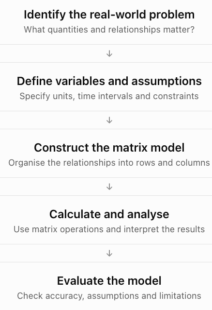
The calculations are only one part of the modelling process. A useful model must also make sense in the context of the original problem.
Transition Matrices
A transition matrix describes how a system changes from one state to another.
Transition matrices are particularly useful when individuals or quantities move between categories over time.
Examples include:
-
Customers switching between brands.
-
Students moving between courses.
-
Animals moving between habitats.
-
Workers changing employment categories.
-
Weather changing between sunny and rainy conditions.
-
Machines changing between operating states.
Understanding states
A state is a category or condition that a system can occupy.
For example, a simple weather model may have two states:
-
Sunny
-
Rainy
Suppose the probabilities of tomorrow's weather are:
|
Today's weather |
Sunny tomorrow |
Rainy tomorrow |
|---|---|---|
|
Sunny |
0.8 |
0.2 |
|
Rainy |
0.3 |
0.7 |
If today is sunny, there is an 80% probability that tomorrow will also be sunny.
If today is rainy, there is a 30% probability that tomorrow will be sunny.
Constructing a transition matrix
In this lesson, we use column state vectors and column-stochastic transition matrices.
This means:
-
Each column represents the current state.
-
Each row represents the next state.
-
Every column sums to 1.
The weather transition matrix is:
The first column represents transitions from sunny weather.
The second column represents transitions from rainy weather.
The columns sum to 1:
0.8 + 0.2 = 1
0.3 + 0.7 = 1
Some textbooks use row-stochastic matrices instead. Both conventions are valid, but the matrix and state-vector orientation must be consistent.
Transition Diagrams
A transition diagram shows states as circles and probabilities as arrows.
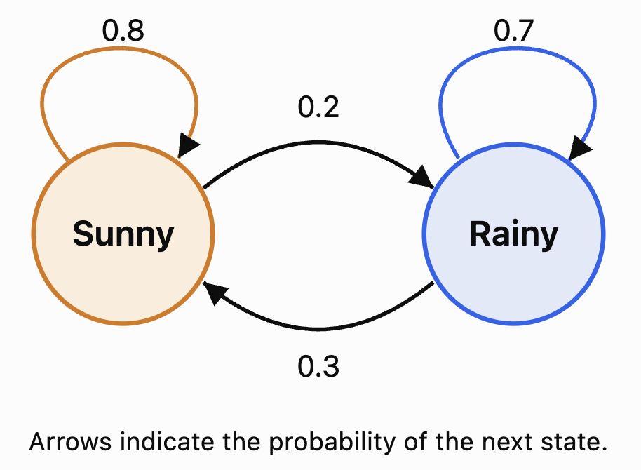
A transition diagram is useful because it provides a visual representation of the same information contained in the matrix.
State Vectors
A state vector describes the current distribution of a system across its states.
For example, suppose the probability of today's weather is:
70% sunny
30% rainy
The state vector is:
To calculate tomorrow's weather probabilities:
More generally:
where:
-
Sₙ is the state vector at time n.
-
T is the transition matrix.
-
Sₙ₊₁ is the state vector at the next time step.
Worked Example 1: Predicting Tomorrow's Weather
Given:
and:
Calculate:
Sunny:
0.8(0.7) + 0.3(0.3) = 0.65
Rainy:
0.2(0.7) + 0.7(0.3) = 0.35
Therefore:
Tomorrow's predicted probabilities are:
-
Sunny: 65%
-
Rainy: 35%
Check:
0.65 + 0.35 = 1
The probabilities are valid.
Repeated Transitions
To predict the state after two time periods:
Since S₁ = TS₀:
Therefore:
After n time periods:
This is one of the most important formulas in transition matrix modelling.
Worked Example 2: Weather After Two Days
Using the previous model:
Calculate:
Sunny:
0.8(0.65) + 0.3(0.35)
= 0.52 + 0.105
= 0.625
Rainy:
0.2(0.65) + 0.7(0.35)
= 0.13 + 0.245
= 0.375
Therefore:
After two days:
-
Sunny probability: 62.5%
-
Rainy probability: 37.5%
The model predicts a gradual movement towards a stable distribution.
Exploring a Transition Model
Use the interactive model below to change the transition probabilities and observe how the state distribution evolves.
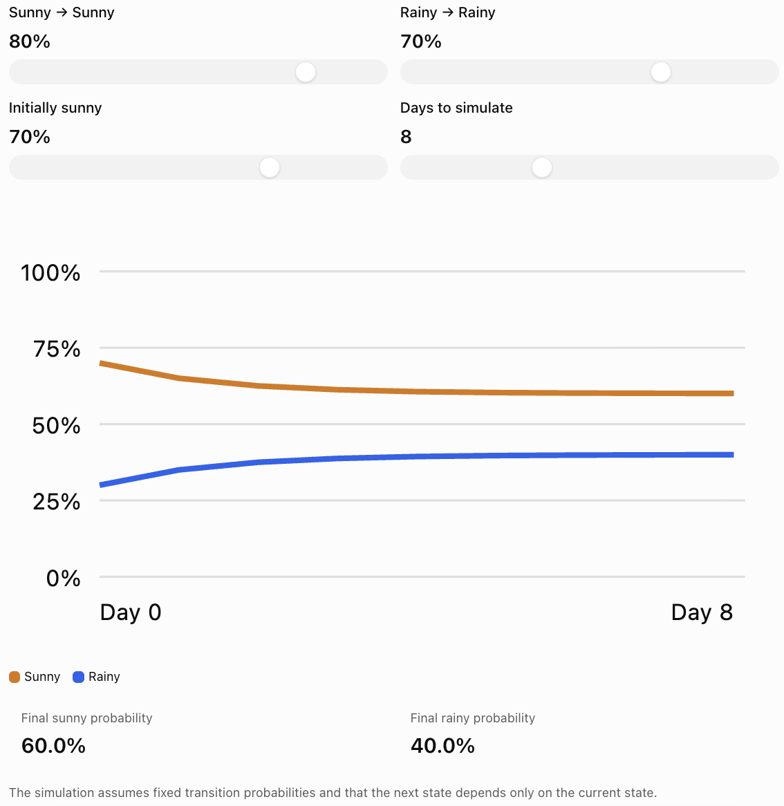
Notice that different starting distributions may approach the same long-term distribution, depending on the transition probabilities.
Steady-State Distributions
A steady-state distribution is a state vector that remains unchanged after applying the transition matrix.
If S is a steady-state vector:
This is also an eigenvector equation with eigenvalue 1.
For a probability transition matrix, the entries of S must be nonnegative and sum to 1.
Worked Example 3: Finding a Steady-State Distribution
Consider:
Let:
We require:
TS = S
Therefore:
0.8x + 0.3y = x
0.2x + 0.7y = y
Rearrange the first equation:
0.3y = 0.2x
Therefore:
3y = 2x
We also know:
x + y = 1
From 3y = 2x:
x = 1.5y
Substitute:
1.5y + y = 1
2.5y = 1
y = 0.4
Then:
x = 0.6
Therefore:
The steady-state distribution is:
-
Sunny: 60%
-
Rainy: 40%
Interpretation
Under this model, the long-term weather distribution approaches 60% sunny and 40% rainy, regardless of the initial probability distribution.
This convergence occurs because the transition matrix has suitable properties, including positive transition probabilities.
Not every transition matrix has a unique steady state or converges to one.
Markov Chains
A Markov chain is a mathematical model describing transitions between states in which the next state depends only on the current state.
This is called the Markov property.
For example, in a simplified weather model, tomorrow's weather depends on today's weather but not directly on the weather several days ago.
A Markov chain consists of:
-
A set of states.
-
Transition probabilities.
-
An initial state or probability distribution.
-
A rule for updating the distribution.
Transition matrices are a convenient way to represent finite Markov chains.
Limitations of Markov models
Real systems may depend on more information than the current state.
For example, weather also depends on:
-
Season
-
Temperature
-
Atmospheric pressure
-
Geographic location
-
Large-scale weather systems
A two-state model is therefore a simplified representation, not a complete weather forecasting system.
Real-World Application 1: Customer Brand Switching
Suppose a market contains two competing brands, A and B.
Each month:
-
85% of Brand A customers remain with A.
-
15% switch from A to B.
-
25% of Brand B customers switch to A.
-
75% remain with B.
The transition matrix is:
Suppose initially:
-
Brand A has 600 customers.
-
Brand B has 400 customers.
The initial state vector is:
Worked Example 4: Predicting Market Shares
Calculate:
Brand A:
0.85(600) + 0.25(400)
= 510 + 100
= 610
Brand B:
0.15(600) + 0.75(400)
= 90 + 300
= 390
Therefore:
After one month, the expected customer counts are:
-
Brand A: 610
-
Brand B: 390
The total remains 1,000.
Long-term interpretation
At steady state:
0.15x = 0.25y
Therefore:
3x = 5y
Since x + y = 1:
x = 0.625
y = 0.375
The long-term market shares are:
-
Brand A: 62.5%
-
Brand B: 37.5%
This assumes customers remain in the two-brand market and the transition probabilities remain constant.
Network Modelling
A network is a collection of objects connected by relationships.
Networks appear in many real-world situations:
-
Cities connected by roads.
-
Airports connected by flights.
-
People connected through social relationships.
-
Computers connected through communication links.
-
Power stations connected by transmission lines.
-
Webpages connected by hyperlinks.
In mathematics, networks are often represented using graphs.
A graph consists of:
-
Vertices (nodes): Objects in the network.
-
Edges: Connections between objects.
Matrices provide an efficient way to represent these connections.
Adjacency Matrices
An adjacency matrix records which vertices in a network are connected.
For a network with n vertices, its adjacency matrix is an n × n matrix.
For a simple undirected graph:
-
Entry 1 indicates a connection.
-
Entry 0 indicates no connection.
-
The matrix is symmetric.
-
Diagonal entries are zero when there are no self-loops.
Example Network
Suppose four locations are connected as follows:
-
A connects to B and C.
-
B connects to A, C, and D.
-
C connects to A and B.
-
D connects only to B.
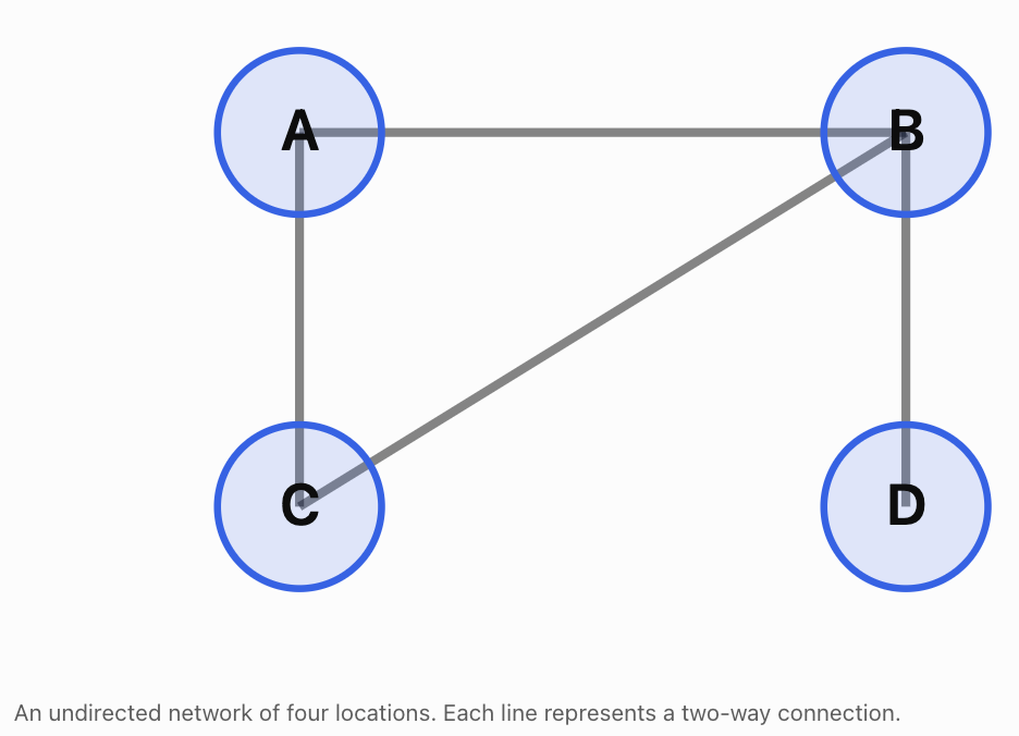
Using the order A, B, C, D, the adjacency matrix is:
\[ \boxed{ M=\begin{bmatrix} 0&1&1&0\\ 1&0&1&1\\ 1&1&0&0\\ 0&1&0&0 \end{bmatrix} } \]Interpreting the matrix
Row A:
0, 1, 1, 0
This means A connects to B and C.
Row B:
1, 0, 1, 1
This means B connects to A, C, and D.
Because the graph is undirected:
Mᵀ = M
The adjacency matrix is symmetric.
Degree of a Vertex
The degree of a vertex is the number of edges connected to it.
For a simple undirected graph, we can calculate the degree by adding the entries in its corresponding adjacency matrix row.
Using the previous network:
Degree of A = 2
Degree of B = 3
Degree of C = 2
Degree of D = 1
Vertex B has the greatest degree.
Therefore, B is the most directly connected vertex in this network.
This type of analysis is useful in transport planning, social networks, and communication systems.
Matrix Powers and Network Paths
An important property of adjacency matrices is that their powers contain information about walks through a network.
If M is the adjacency matrix of a graph, then:
The entry (i, j) of Mⁿ counts the number of walks of length n from vertex i to vertex j.
A walk may revisit vertices or edges, so it is not necessarily a simple path.
Worked Example 5: Counting Two-Step Walks
Consider a network with three vertices:
A — B — C
Its adjacency matrix is:
\[ M=\begin{bmatrix} 0&1&0\\ 1&0&1\\ 0&1&0 \end{bmatrix} \]Calculate M²:
\[ M^2= \begin{bmatrix} 0&1&0\\ 1&0&1\\ 0&1&0 \end{bmatrix} \begin{bmatrix} 0&1&0\\ 1&0&1\\ 0&1&0 \end{bmatrix} \]The result is:
\[ \boxed{ M^2=\begin{bmatrix} 1&0&1\\ 0&2&0\\ 1&0&1 \end{bmatrix} } \]Interpret the entry in row A, column C.
It equals 1.
Therefore, there is exactly one two-step walk from A to C:
A → B → C
The entry in row B, column B equals 2.
There are two two-step walks from B back to B:
B → A → B
B → C → B
This demonstrates how matrix multiplication can reveal indirect connections.
Directed Networks
Some networks contain connections that operate in only one direction.
Examples include:
-
One-way roads.
-
Flights operating in one direction.
-
Social media following relationships.
-
Webpage hyperlinks.
-
Supply chains.
These are called directed graphs.
For a directed graph, the adjacency matrix does not need to be symmetric.
Suppose:
A → B
B → C
C → A
The adjacency matrix is:
\[ M=\begin{bmatrix} 0&1&0\\ 0&0&1\\ 1&0&0 \end{bmatrix} \]Here, rows represent starting vertices and columns represent destination vertices.
For example:
M₁₂ = 1
means there is a directed edge from A to B.
But:
M₂₁ = 0
means there is no directed edge from B to A.
The direction of connections matters.
Weighted Networks
Not all connections are equally important.
Some networks assign numerical values to edges.
These values are called weights.
Weights may represent:
-
Distance
-
Travel time
-
Cost
-
Capacity
-
Strength of a relationship
-
Amount of information transferred
Example: Transport Network
Suppose three cities are connected by roads.
Route
Distance
A to B
40 km
A to C
70 km
B to C
30 km
A weighted adjacency matrix is:
\[ W=\begin{bmatrix} 0&40&70\\ 40&0&30\\ 70&30&0 \end{bmatrix} \]The entry in row A, column B is 40, indicating a distance of 40 km.
For this particular network, zero on the diagonal represents the distance from a city to itself.
When zero is also used to represent no connection, care is needed to distinguish missing routes from zero-weight routes.
Why weighted networks are useful
They allow us to investigate:
-
Shortest routes.
-
Lowest-cost connections.
-
Transport efficiency.
-
Communication capacity.
-
Resource distribution.
However, ordinary matrix multiplication does not directly calculate shortest routes. Shortest-path problems generally require specialised algorithms or alternative matrix operations.
Real-World Application 2: School Course Enrolment
A school offers three elective courses:
-
Art
-
Music
-
Technology
At the beginning of a semester, enrolment is:
Course
Students
Art
80
Music
60
Technology
100
The initial enrolment vector is:
\[ S_0=\begin{bmatrix}80\\60\\100\end{bmatrix} \]Suppose the school estimates the following transition percentages between semesters.
Current course
Next: Art
Next: Music
Next: Technology
Art
70%
20%
10%
Music
10%
80%
10%
Technology
20%
10%
70%
Using our column-vector convention, the transition matrix is:
\[ T=\begin{bmatrix} 0.7&0.1&0.2\\ 0.2&0.8&0.1\\ 0.1&0.1&0.7 \end{bmatrix} \]Worked Example 6: Predicting Enrolment
Calculate:
\[ S_1=TS_0 \]\[ S_1= \begin{bmatrix} 0.7&0.1&0.2\\ 0.2&0.8&0.1\\ 0.1&0.1&0.7 \end{bmatrix} \begin{bmatrix} 80\\60\\100 \end{bmatrix} \]Art:
0.7(80) + 0.1(60) + 0.2(100)
= 56 + 6 + 20
= 82
Music:
0.2(80) + 0.8(60) + 0.1(100)
= 16 + 48 + 10
= 74
Technology:
0.1(80) + 0.1(60) + 0.7(100)
= 8 + 6 + 70
= 84
Therefore:
\[ \boxed{S_1=\begin{bmatrix}82\\74\\84\end{bmatrix}} \]Interpretation
The model predicts:
-
Art: 82 students
-
Music: 74 students
-
Technology: 84 students
The total remains:
82 + 74 + 84 = 240
This agrees with the original total of 240 students.
Evaluating the model
The model assumes:
-
Students select exactly one of these electives.
-
No students enter or leave the group.
-
The transition probabilities remain constant.
-
Student decisions can be represented using the estimated percentages.
In reality, course popularity, teacher availability, timetabling, and student preferences may change.
Therefore, the predictions should be treated as estimates.
Real-World Application 3: Input–Output Economic Models
Matrices can describe how different industries depend on one another.
For example, agriculture may require manufacturing products, while manufacturing may require agricultural resources.
These relationships can be represented using an input–output model.
Suppose an economy has two industries:
-
Agriculture
-
Manufacturing
For each unit of agricultural output, production requires:
-
0.2 units of agricultural output.
-
0.1 units of manufacturing output.
For each unit of manufacturing output, production requires:
-
0.3 units of agricultural output.
-
0.2 units of manufacturing output.
The input coefficient matrix is:
\[ A=\begin{bmatrix} 0.2&0.3\\ 0.1&0.2 \end{bmatrix} \]The columns represent the industries producing output, while the rows represent the inputs required.
Suppose final consumer demand is:
\[ D=\begin{bmatrix}100\\80\end{bmatrix} \]Let X represent the total production required.
The model is:
\[ X=AX+D \]Rearrange:
\[ X-AX=D \]\[ (I-A)X=D \]Therefore:
\[ \boxed{X=(I-A)^{-1}D} \]provided I − A is invertible.
Worked Example 7: Calculating Required Production
First:
\[ I-A= \begin{bmatrix} 0.8&-0.3\\ -0.1&0.8 \end{bmatrix} \]Calculate the determinant:
det(I − A) = 0.8(0.8) − (−0.3)(−0.1)
= 0.64 − 0.03
= 0.61
Therefore:
\[ (I-A)^{-1}= \frac1{0.61} \begin{bmatrix} 0.8&0.3\\ 0.1&0.8 \end{bmatrix} \]Multiply:
\[ X=\frac1{0.61} \begin{bmatrix} 0.8&0.3\\ 0.1&0.8 \end{bmatrix} \begin{bmatrix}100\\80\end{bmatrix} \]\[ X=\frac1{0.61} \begin{bmatrix} 104\\74 \end{bmatrix} \]Therefore:
\[ \boxed{ X\approx\begin{bmatrix} 170.49\\ 121.31 \end{bmatrix} } \]The economy must produce approximately:
-
170.49 units of agricultural output.
-
121.31 units of manufacturing output.
These totals exceed final consumer demand because each industry also supplies inputs needed for production.
This simplified model assumes fixed input requirements and sufficient production capacity.
Analysing Matrix-Based Systems
Once a matrix model has been constructed, we can investigate more than its immediate numerical results.
We can examine its stability, sensitivity, connectivity, and long-term behaviour.
Stability
A system is stable when its behaviour remains controlled or approaches a predictable state.
For a repeated linear system:
\[ X_{n+1}=AX_n \]the magnitudes of eigenvalues help determine long-term behaviour.
-
Eigenvalues with absolute value less than 1 correspond to directions that decay.
-
Eigenvalues with absolute value greater than 1 correspond to directions that grow.
-
Eigenvalues with absolute value equal to 1 require closer analysis.
If all eigenvalues have absolute value less than 1, then repeated application of A drives every state vector towards zero.
Transition matrices behave differently because they have an eigenvalue of 1, and may approach a nonzero steady-state distribution.
Sensitivity
A model is sensitive when small changes in inputs or assumptions produce large changes in its predictions.
For example, changing a customer retention rate from 85% to 80% may affect long-term market shares substantially.
Sensitivity analysis helps answer questions such as:
-
What happens if costs increase?
-
What happens if transition probabilities change?
-
What happens if demand rises?
-
Which assumptions have the greatest influence?
Connectivity
In network models, we can investigate how well the system is connected.
Useful measurements include:
-
Degree of a vertex.
-
Number of walks between vertices.
-
Whether one vertex can be reached from another.
-
Importance of particular connections.
-
Whether removing an edge disconnects part of the network.
Model validity
A matrix calculation may be mathematically correct but still produce a poor real-world prediction.
A model should be evaluated by asking:
-
Are the assumptions realistic?
-
Are the input values reliable?
-
Are the units consistent?
-
Are important factors missing?
-
Does the model agree with observed data?
-
How far into the future can the predictions reasonably be trusted?
Worked Example 8: Evaluating a Population Model
A population contains two groups of animals.
The population changes according to:
\[ X_{n+1}= \begin{bmatrix} 0.8&0\\ 0&1.2 \end{bmatrix}X_n \]Initially:
\[ X_0=\begin{bmatrix}100\\50\end{bmatrix} \]Calculate the population after two periods.
Step 1: Calculate the first period.
\[ X_1= \begin{bmatrix} 0.8&0\\ 0&1.2 \end{bmatrix} \begin{bmatrix}100\\50\end{bmatrix} \]\[ X_1=\begin{bmatrix}80\\60\end{bmatrix} \]Step 2: Calculate the second period.
\[ X_2= \begin{bmatrix} 0.8&0\\ 0&1.2 \end{bmatrix} \begin{bmatrix}80\\60\end{bmatrix} \]\[ \boxed{X_2=\begin{bmatrix}64\\72\end{bmatrix}} \]Interpretation
The first group decreases by 20% each period.
The second group increases by 20% each period.
The eigenvalues are:
λ₁ = 0.8
λ₂ = 1.2
These values explain the different long-term behaviours.
Limitations
The model assumes fixed growth rates and no interaction between the groups.
Real populations may be affected by food availability, disease, migration, competition, and environmental changes.
Choosing an Appropriate Matrix Model
Different problems require different types of matrices.
Situation
Suitable model
Calculating resources for production
Resource coefficient matrix
Predicting movement between categories
Transition matrix
Representing connections between locations
Adjacency matrix
Representing distances or costs
Weighted network matrix
Analysing relationships between industries
Input–output matrix
Predicting repeated growth or decay
Repeated matrix transformation
Finding long-term probability distributions
Steady-state transition model
The most important modelling decision is identifying what the rows, columns, and matrix entries represent.
A well-constructed matrix model should have a clear interpretation for every entry.
Common Mistakes
Mistake 1: Reversing rows and columns in a transition matrix
Always establish whether rows or columns represent the current state.
Mistake 2: Forgetting that transition probabilities must sum to 1
Under the column-stochastic convention, each column must sum to 1.
Mistake 3: Multiplying matrices in the wrong order
For column state vectors, use Sₙ₊₁ = TSₙ.
Mistake 4: Confusing a state vector with a transition matrix
The state vector describes the current distribution. The transition matrix describes how that distribution changes.
Mistake 5: Assuming all transition matrices converge to one steady state
Some systems cycle or have multiple steady states.
Mistake 6: Confusing paths and walks
Matrix powers count walks, which may revisit vertices or edges.
Mistake 7: Assuming adjacency matrices must be symmetric
Only undirected networks have symmetric adjacency matrices under the standard convention.
Mistake 8: Confusing weighted networks with ordinary adjacency matrices
Weighted matrices contain values such as distances or costs, not simply zeros and ones.
Mistake 9: Ignoring units
A resource matrix may contain hours, kilograms, or monetary amounts. These must be interpreted consistently.
Mistake 10: Assuming model predictions are guaranteed outcomes
Models describe expected or estimated behaviour based on assumptions.
Mistake 11: Applying matrix operations without checking dimensions
Matrix multiplication requires compatible dimensions.
Mistake 12: Ignoring model limitations
Real systems may contain factors not represented by the matrix.
Key Terms
-
Matrix Model: Mathematical representation of a system using matrices.
-
State: Category or condition occupied by a system.
-
State Vector: Vector describing the current distribution across states.
-
Transition Matrix: Matrix describing movement between states.
-
Transition Probability: Probability of moving from one state to another.
-
Column-Stochastic Matrix: Nonnegative matrix whose columns each sum to 1.
-
Row-Stochastic Matrix: Nonnegative matrix whose rows each sum to 1.
-
Markov Chain: Model in which the next state depends only on the current state.
-
Markov Property: Assumption that future transitions depend only on the present state.
-
Steady-State Distribution: Probability distribution unchanged by the transition matrix.
-
Matrix Power: Repeated multiplication of a matrix by itself.
-
Network: Collection of objects connected by relationships.
-
Graph: Mathematical structure consisting of vertices and edges.
-
Vertex: Node representing an object in a network.
-
Edge: Connection between two vertices.
-
Adjacency Matrix: Matrix recording connections between vertices.
-
Directed Graph: Graph whose edges have directions.
-
Undirected Graph: Graph whose edges do not have directions.
-
Weighted Graph: Graph whose edges have numerical values.
-
Degree: Number of edges incident to a vertex in an undirected graph.
-
Walk: Sequence of connected vertices that may repeat vertices or edges.
-
Path: Walk with no repeated vertices, under the standard simple-path definition.
-
Connectivity: Description of how vertices are linked.
-
Input–Output Model: Economic model describing relationships between industries.
-
Eigenvalue: Scalar describing how an eigenvector is scaled.
-
Stability: Behaviour of a system over time.
-
Sensitivity Analysis: Investigation of how changes in inputs affect outputs.
-
Model Assumption: Simplification or condition used to construct a model.
-
Model Validation: Process of comparing a model with real-world observations.
Key Takeaways
-
Matrices can represent practical systems involving several related quantities.
-
Matrix multiplication can calculate resource requirements and other outputs.
-
Transition matrices describe movement between states.
-
State vectors represent the current distribution of a system.
-
Repeated transitions are calculated using Sₙ = TⁿS₀.
-
A steady-state distribution satisfies TS = S.
-
Markov chains describe transitions that depend only on the current state.
-
Networks can be represented using adjacency matrices.
-
Matrix powers can count walks of specified lengths in a network.
-
Directed networks may have non-symmetric adjacency matrices.
-
Weighted networks represent quantities such as distance, cost, or capacity.
-
Matrix models can describe population changes, market shares, and economic relationships.
-
Eigenvalues help explain growth, decay, and stability.
-
Mathematical models depend on assumptions and may not perfectly represent reality.
-
Results must always be interpreted in the context of the original problem.
Check Your Understanding
Questions
Question 1: Resource Modelling
A factory produces two products.
Product A requires 3 labour hours and 4 material units.
Product B requires 5 labour hours and 2 material units.
Write the resource matrix.
Question 2: Matrix Multiplication
Using Question 1, calculate the resources required to produce 10 units of A and 20 units of B.
Question 3: Transition Matrix
A system has two states, A and B.
-
80% of A remains in A.
-
20% of A moves to B.
-
30% of B moves to A.
-
70% of B remains in B.
Write the column-stochastic transition matrix.
Question 4: One-Step Transition
Using Question 3, calculate the next state if:
\[ S_0=\begin{bmatrix}100\\200\end{bmatrix} \]Question 5: Two-Step Transition
Using the same transition matrix and initial state, calculate S₂.
Question 6: Steady State
Find the steady-state probability distribution for:
\[ T=\begin{bmatrix} 0.7&0.2\\ 0.3&0.8 \end{bmatrix} \]Question 7: Adjacency Matrix
A network contains three vertices:
A connects to B.
B connects to A and C.
C connects to B.
Write its adjacency matrix.
Question 8: Vertex Degree
Using Question 7, determine the degree of each vertex.
Question 9: Matrix Powers
Calculate M² for the adjacency matrix in Question 7.
Interpret the entry in row A, column C.
Question 10: Directed Network
A directed network has connections:
A → B
B → C
C → A
Write its adjacency matrix.
Question 11: Weighted Network
Three cities have the following direct road distances:
A–B: 50 km
A–C: 80 km
B–C: 40 km
Write a symmetric weighted adjacency matrix.
Question 12: Population Model
A population is modelled by:
\[ X_{n+1}= \begin{bmatrix} 0.9&0\\ 0&1.1 \end{bmatrix}X_n \]If:
\[ X_0=\begin{bmatrix}200\\100\end{bmatrix} \]calculate X₂.
Question 13: Economic Modelling
An economy has:
\[ A=\begin{bmatrix} 0.2&0\\ 0&0.25 \end{bmatrix} \]and final demand:
\[ D=\begin{bmatrix}80\\60\end{bmatrix} \]Solve X = AX + D.
Question 14: Evaluating Models
Explain three limitations of using a fixed transition matrix to predict customer behaviour over several years.
Question 15: Integrated Challenge
A school has 500 students choosing between two clubs, Science and Mathematics.
Initially:
-
300 students choose Science.
-
200 students choose Mathematics.
Each semester:
-
80% of Science students remain in Science.
-
20% move to Mathematics.
-
30% of Mathematics students move to Science.
-
70% remain in Mathematics.
a) Construct the transition matrix.
b) Write the initial state vector.
c) Calculate the expected club membership after one semester.
d) Calculate the expected membership after two semesters.
e) Find the steady-state distribution.
f) Explain two assumptions of the model.
Fully Worked Answers
Answer 1: Resource Modelling
Rows represent labour and materials.
Columns represent Products A and B.
\[ \boxed{ R=\begin{bmatrix} 3&5\\ 4&2 \end{bmatrix} } \]Answer 2: Matrix Multiplication
Production vector:
\[ P=\begin{bmatrix}10\\20\end{bmatrix} \]Calculate:
\[ RP= \begin{bmatrix} 3&5\\ 4&2 \end{bmatrix} \begin{bmatrix}10\\20\end{bmatrix} \]Labour:
3(10) + 5(20) = 130
Materials:
4(10) + 2(20) = 80
\[ \boxed{RP=\begin{bmatrix}130\\80\end{bmatrix}} \]Answer: 130 labour hours and 80 material units.
Answer 3: Transition Matrix
Using columns for current states:
\[ \boxed{ T=\begin{bmatrix} 0.8&0.3\\ 0.2&0.7 \end{bmatrix} } \]Each column sums to 1.
Answer 4: One-Step Transition
\[ S_1=TS_0 \]\[ S_1= \begin{bmatrix} 0.8&0.3\\ 0.2&0.7 \end{bmatrix} \begin{bmatrix}100\\200\end{bmatrix} \]First component:
0.8(100) + 0.3(200) = 140
Second component:
0.2(100) + 0.7(200) = 160
\[ \boxed{S_1=\begin{bmatrix}140\\160\end{bmatrix}} \]Answer 5: Two-Step Transition
Use the result from Question 4:
\[ S_1=\begin{bmatrix}140\\160\end{bmatrix} \]Then:
\[ S_2=TS_1 \]First component:
0.8(140) + 0.3(160) = 160
Second component:
0.2(140) + 0.7(160) = 140
\[ \boxed{S_2=\begin{bmatrix}160\\140\end{bmatrix}} \]Answer 6: Steady State
Given:
\[ T=\begin{bmatrix}0.7&0.2\\0.3&0.8\end{bmatrix} \]Let:
\[ S=\begin{bmatrix}x\\y\end{bmatrix} \]Solve:
TS = S
From the first row:
0.7x + 0.2y = x
Therefore:
0.2y = 0.3x
2y = 3x
y = 1.5x
Also:
x + y = 1
Therefore:
x + 1.5x = 1
2.5x = 1
x = 0.4
y = 0.6
\[ \boxed{S=\begin{bmatrix}0.4\\0.6\end{bmatrix}} \]Answer: 40% in A and 60% in B.
Answer 7: Adjacency Matrix
Connections:
A–B
B–C
The adjacency matrix is:
\[ \boxed{ M=\begin{bmatrix} 0&1&0\\ 1&0&1\\ 0&1&0 \end{bmatrix} } \]Answer 8: Vertex Degree
Add the entries in each row.
A: 0 + 1 + 0 = 1
B: 1 + 0 + 1 = 2
C: 0 + 1 + 0 = 1
Answer: Degree(A) = 1, Degree(B) = 2, Degree(C) = 1.
Answer 9: Matrix Powers
\[ M=\begin{bmatrix} 0&1&0\\ 1&0&1\\ 0&1&0 \end{bmatrix} \]Multiplying M by itself gives:
\[ \boxed{ M^2=\begin{bmatrix} 1&0&1\\ 0&2&0\\ 1&0&1 \end{bmatrix} } \]The entry in row A, column C equals 1.
Therefore, there is one two-step walk from A to C:
A → B → C
Answer 10: Directed Network
Using rows as starting vertices and columns as destinations:
\[ \boxed{ M=\begin{bmatrix} 0&1&0\\ 0&0&1\\ 1&0&0 \end{bmatrix} } \]This matrix is not symmetric because the connections are directed.
Answer 11: Weighted Network
Using the order A, B, C:
\[ \boxed{ W=\begin{bmatrix} 0&50&80\\ 50&0&40\\ 80&40&0 \end{bmatrix} } \]The matrix is symmetric because the distances are the same in both directions.
Answer 12: Population Model
Given:
\[ A=\begin{bmatrix}0.9&0\\0&1.1\end{bmatrix} \]and:
\[ X_0=\begin{bmatrix}200\\100\end{bmatrix} \]After one period:
\[ X_1=\begin{bmatrix}180\\110\end{bmatrix} \]After two periods:
\[ X_2=AX_1 \]\[ X_2= \begin{bmatrix} 0.9(180)\\ 1.1(110) \end{bmatrix} \]\[ \boxed{X_2=\begin{bmatrix}162\\121\end{bmatrix}} \]The first group decreases while the second increases.
Answer 13: Economic Modelling
Given:
\[ A=\begin{bmatrix}0.2&0\\0&0.25\end{bmatrix} \]and:
\[ D=\begin{bmatrix}80\\60\end{bmatrix} \]The model is:
X = AX + D
Therefore:
(I − A)X = D
\[ I-A=\begin{bmatrix}0.8&0\\0&0.75\end{bmatrix} \]This gives:
0.8x = 80
0.75y = 60
Therefore:
x = 100
y = 80
\[ \boxed{X=\begin{bmatrix}100\\80\end{bmatrix}} \]Answer 14: Evaluating Models
Three limitations include:
-
Changing preferences: Customer choices may change because of advertising, prices, or new products.
-
Fixed probabilities: The model assumes transition probabilities remain constant, which may be unrealistic over several years.
-
Missing factors: Economic conditions, competitors, and population changes may affect customer behaviour.
Therefore, predictions become less reliable if the model assumptions no longer reflect reality.
Answer 15: Integrated Challenge
Part a: Transition matrix
Using Science first and Mathematics second:
\[ \boxed{ T=\begin{bmatrix} 0.8&0.3\\ 0.2&0.7 \end{bmatrix} } \]Part b: Initial state vector
\[ \boxed{ S_0=\begin{bmatrix}300\\200\end{bmatrix} } \]Part c: After one semester
\[ S_1=TS_0 \]Science:
0.8(300) + 0.3(200)
= 240 + 60
= 300
Mathematics:
0.2(300) + 0.7(200)
= 60 + 140
= 200
Therefore:
\[ \boxed{S_1=\begin{bmatrix}300\\200\end{bmatrix}} \]The membership distribution remains unchanged.
Part d: After two semesters
Since S₁ = S₀:
\[ S_2=TS_1 \]\[ \boxed{S_2=\begin{bmatrix}300\\200\end{bmatrix}} \]The distribution remains unchanged again.
Part e: Steady-state distribution
Let:
\[ S=\begin{bmatrix}x\\y\end{bmatrix} \]Solve:
TS = S
From the first row:
0.8x + 0.3y = x
Therefore:
0.3y = 0.2x
3y = 2x
x = 1.5y
Since:
x + y = 1
1.5y + y = 1
2.5y = 1
y = 0.4
x = 0.6
Therefore:
\[ \boxed{S=\begin{bmatrix}0.6\\0.4\end{bmatrix}} \]The steady-state distribution is:
-
Science: 60%
-
Mathematics: 40%
For 500 students:
Science = 0.6(500) = 300
Mathematics = 0.4(500) = 200
The initial distribution was already at steady state.
Part f: Assumptions
Two assumptions are:
-
The total number of students remains constant at 500.
-
The transition percentages remain unchanged each semester.
Other assumptions include that students belong to exactly one of the two clubs and that movement depends only on their current club.
Final Reflection
Matrix modelling allows complex real-world systems to be represented using organised mathematical structures.
Transition matrices describe movement between categories, while adjacency matrices represent connections within networks. Weighted matrices extend these ideas by including distances, costs, capacities, and other numerical relationships.
Matrix multiplication allows us to predict future states, calculate resource requirements, and analyse indirect network connections.
Repeated matrix operations reveal how systems change over time, while steady-state analysis and eigenvalues help explain long-term behaviour.
However, mathematical modelling requires more than correct calculations. A useful model must be based on reasonable assumptions, interpreted carefully, and evaluated against real-world evidence.
The central idea is that matrices transform complicated relationships into mathematical models that can be used to describe systems, analyse their behaviour, make predictions, and support practical decisions.
-
4. Computer Graphics and Robotics
Learning outcomes
- I can explain how matrices are used in computer graphics.
- I can model object transformations.
- I can describe robotic movement using matrices.
- I can analyse simple graphical transformations.
- I can recognise applications in technology.
Introduction
Every time a video game character moves, a 3D model rotates, or a robot arm reaches for an object, mathematics is working behind the scenes.
Computer graphics and robotics rely heavily on matrices to describe positions, movements, rotations, reflections, enlargements, and changes in perspective.
A computer-generated object may contain thousands or millions of points. Rather than calculating the movement of every point separately using different formulas, computers use matrix transformations to apply consistent mathematical operations efficiently.
Similarly, robots use matrices to describe the positions and orientations of their components. When a robotic arm rotates at a joint, the positions of all attached components change. Matrix multiplication allows engineers to calculate these changes systematically.
Matrices are used in:
-
Video games and computer animation.
-
Three-dimensional modelling and rendering.
-
Virtual reality and augmented reality.
-
Industrial robotic arms.
-
Autonomous vehicles and drones.
-
Medical imaging and robotic surgery.
-
Computer vision and object tracking.
-
Satellite navigation and aerospace engineering.
In this lesson, we will investigate how matrices represent graphical transformations, how transformations can be combined, and how similar mathematical techniques are used to control robotic movement.
How Computers Represent Objects
A computer graphic can be represented using a collection of points called vertices.
In two dimensions, each vertex has coordinates:
For example, a triangle may have vertices:
A = (1, 1)
B = (4, 1)
C = (2, 3)
These vertices determine the shape of the triangle.
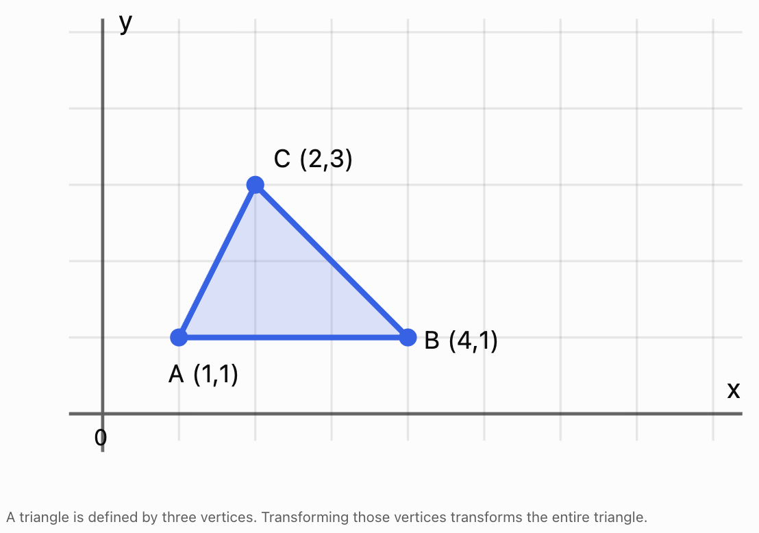
We can organise the coordinates into a matrix:
Each column represents one vertex.
If T is a 2 × 2 transformation matrix, the transformed vertices are:
This means one matrix multiplication can transform every vertex of the object.
For a 3D object, vertices have three coordinates:
A 3 × 3 matrix can then represent rotations, reflections, scaling, and shears in three-dimensional space.
Matrix Transformations in Computer Graphics
A transformation changes the position, size, shape, or orientation of an object.
Common transformations include:
|
Transformation |
Effect |
|---|---|
|
Translation |
Moves an object |
|
Rotation |
Turns an object |
|
Reflection |
Flips an object |
|
Enlargement |
Increases its size |
|
Reduction |
Decreases its size |
|
Shear |
Slants or distorts its shape |
Most of these transformations can be represented by 2 × 2 matrices when they are performed about the origin.
Translations require a different approach, which we will investigate using homogeneous coordinates.
Rotation Matrices
A rotation turns an object through a specified angle about a fixed point.
For a counterclockwise rotation through angle θ about the origin:
For a point P:
Common Rotation Matrices
A 90° counterclockwise rotation:
A 180° rotation:
A 270° counterclockwise rotation:
A clockwise rotation through θ is equivalent to a counterclockwise rotation through −θ.
Worked Example 1: Rotating a Point
Rotate P = (3, 2) by 90° counterclockwise about the origin.
Use:
Then:
Therefore:
The point has rotated 90° counterclockwise while remaining the same distance from the origin.
Worked Example 2: Rotating an Entire Triangle
Consider the triangle:
A = (1, 1)
B = (3, 1)
C = (2, 3)
Its vertex matrix is:
Apply a 90° counterclockwise rotation:
The result is:
Therefore:
A′ = (−1, 1)
B′ = (−1, 3)
C′ = (−3, 2)
The triangle has rotated without changing its side lengths or angles.
Reflection Matrices
A reflection flips an object across a specified line.
Reflection in the x-axis
This maps:
(x, y) → (x, −y)
Reflection in the y-axis
This maps:
(x, y) → (−x, y)
Reflection in the line y = x
This maps:
(x, y) → (y, x)
Worked Example 3: Reflecting a Point
Reflect P = (4, −2) in the y-axis.
The reflected point is (−4, −2).
Reflections preserve lengths and angles but reverse orientation.
Scaling Matrices
Scaling changes the size of an object.
A general two-dimensional scaling matrix is:
where:
-
sₓ is the horizontal scale factor.
-
sᵧ is the vertical scale factor.
If sₓ = sᵧ, the scaling is uniform.
If sₓ and sᵧ are different, the scaling is non-uniform.
Worked Example 4: Non-Uniform Scaling
A point P = (2, 3) is scaled horizontally by factor 3 and vertically by factor 2.
Then:
The new point is (6, 6).
Non-uniform scaling may distort the proportions of an object.
Uniform scaling preserves its shape.
Shear Transformations
A shear transformation slants an object.
A horizontal shear has the form:
This maps:
(x, y) → (x + ky, y)
A vertical shear has the form:
This maps:
(x, y) → (x, kx + y)
Worked Example 5: Horizontal Shear
Apply a horizontal shear with k = 2 to P = (1, 3).
Therefore:
The y-coordinate remains unchanged, while the x-coordinate increases.
Exploring Graphical Transformations
Change the transformation and observe how a square is altered.
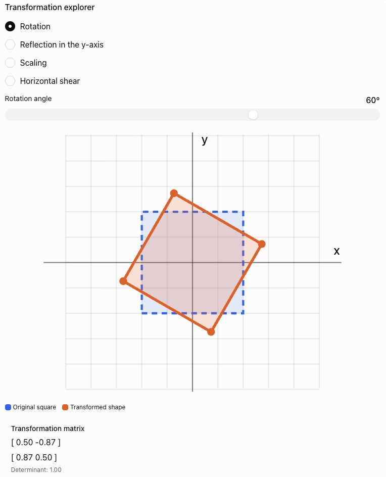
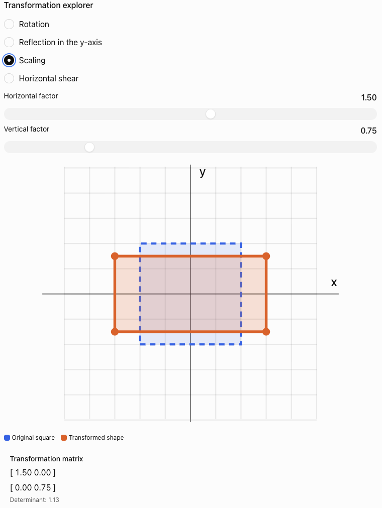
Observe how the determinant relates to the area and orientation of the transformed shape.
Combining Transformations
Computer graphics often requires several transformations to be applied to the same object.
For example, a character may need to:
-
Rotate.
-
Enlarge.
-
Move to a new position.
Matrix multiplication allows these operations to be combined.
Suppose A is applied first, followed by B.
Then:
Therefore:
The order of matrix multiplication is important.
In general:
Worked Example 6: Rotation Followed by Scaling
Consider:
First rotate 90° counterclockwise:
Then scale horizontally by factor 2:
The combined transformation is:
Calculate:
Apply to P:
Reversing the Order
Now scale first and rotate second.
Therefore:
The results differ:
-
Rotation then scaling: (−4, 1)
-
Scaling then rotation: (−2, 2)
This demonstrates why transformation order must be handled carefully.
Translation and Homogeneous Coordinates
A translation moves every point by the same amount.
For a point (x, y), a translation by (a, b) gives:
A standard 2 × 2 matrix cannot represent a nonzero translation because matrix multiplication maps the origin to itself.
Computer graphics solves this problem using homogeneous coordinates.
A two-dimensional point is represented using three coordinates:
A translation becomes:
Then:
This allows translation, rotation, scaling, and other affine transformations to be combined using matrix multiplication.
Worked Example 7: Translating a Point
Translate P = (2, 3) by 4 units right and 2 units down.
Therefore:
a = 4
b = −2
Apply the transformation:
Therefore:
Homogeneous Transformation Matrices
Using homogeneous coordinates, a general two-dimensional affine transformation can be written as:
The upper-left 2 × 2 block describes the linear transformation.
The final column describes translation.
This structure is extremely useful in computer graphics and robotics.
For example, a rotation followed by a translation can be represented using a single 3 × 3 matrix.
Worked Example 8: Rotation and Translation
Rotate a point by 90° counterclockwise, then translate it 5 units right and 2 units up.
The combined matrix is:
Apply it to P = (2, 1):
Therefore:
We can verify the result manually.
Rotate:
(2, 1) → (−1, 2)
Translate:
(−1 + 5, 2 + 2) = (4, 4)
The results agree.
Three-Dimensional Computer Graphics
Realistic computer graphics usually operates in three dimensions.
A 3D point has coordinates:
Three-dimensional rotations can occur around the x-axis, y-axis, or z-axis.
Rotation Around the x-Axis
Rotation Around the y-Axis
Rotation Around the z-Axis
These formulas use the usual right-handed coordinate system and the right-hand rule for positive rotations.
Worked Example 9: Rotating in Three Dimensions
Consider:
Rotate 90° counterclockwise around the z-axis, as viewed from the positive z-axis towards the origin.
Then:
The z-coordinate remains unchanged because the rotation occurs around the z-axis.
How Matrices Are Used in Robotics
Robotics uses many of the same mathematical ideas as computer graphics.
A robot must understand:
-
Where it is located.
-
Which direction it is facing.
-
How its joints are positioned.
-
Where its tools or sensors are located.
-
How to move from one position to another.
Matrices provide a consistent mathematical method for describing these relationships.
Coordinate Frames
A coordinate frame defines a position and orientation from which measurements are made.
A robot may use several coordinate frames:
-
World frame: fixed reference for the environment.
-
Robot base frame: attached to the robot's base.
-
Joint frames: attached to moving joints.
-
Tool frame: attached to the robot's end effector.
The end effector is the part of a robot that performs a task, such as a gripper, welding tool, or surgical instrument.
Transformations allow coordinates to be converted from one frame to another.
Modelling a Simple Robotic Arm
Consider a robotic arm operating in a two-dimensional plane.
The arm has two segments:
-
First segment of length L₁.
-
Second segment of length L₂.
The first joint rotates through angle θ₁.
The second joint rotates through angle θ₂ relative to the first segment.
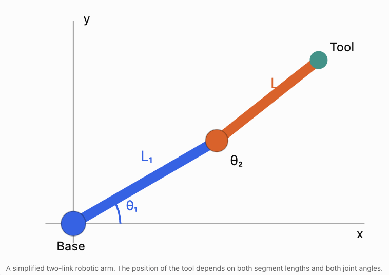
The end effector's position can be calculated using trigonometry.
These equations are examples of forward kinematics.
Forward kinematics calculates the position of the robot's end effector from known joint angles and link lengths.
Worked Example 10: Position of a Robotic Arm
A robot has:
L₁ = 4 m
L₂ = 3 m
θ₁ = 30°
θ₂ = 60°
Calculate the position of the end effector.
Step 1: Calculate the horizontal position.
Using:
cos 30° ≈ 0.866
cos 90° = 0
Therefore:
x = 4(0.866) + 3(0)
x ≈ 3.464 m
Step 2: Calculate the vertical position.
Using:
sin 30° = 0.5
sin 90° = 1
Therefore:
y = 4(0.5) + 3(1)
y = 2 + 3
y = 5 m
Therefore:
The end effector is approximately 3.464 m horizontally and 5 m vertically from the robot's base.
Forward Kinematics Using Matrices
The same robotic arm can be modelled using homogeneous transformation matrices.
For a planar rotation θ followed by movement of length L along the rotated local x-axis:
For a two-link arm:
where:
and:
The total transformation describes the end effector's position and orientation relative to the robot's base.
The resulting matrix is:
where:
x = L₁ cos θ₁ + L₂ cos(θ₁ + θ₂)
y = L₁ sin θ₁ + L₂ sin(θ₁ + θ₂)
This method becomes especially useful for robots with many joints.
Instead of constructing a separate set of trigonometric equations for every possible configuration, engineers multiply transformation matrices representing individual joints.
Inverse Kinematics
Inverse kinematics works in the opposite direction from forward kinematics.
Forward kinematics asks:
Given the joint angles, where is the end effector?
Inverse kinematics asks:
Given a desired end-effector position, what joint angles are required?
For example, a robotic arm may need to pick up an object at coordinates (5, 2).
The robot must calculate joint angles that position its gripper at that location.
Inverse kinematics is generally more difficult because:
-
Some target positions may be unreachable.
-
Multiple joint configurations may reach the same position.
-
Some configurations may cause collisions.
-
Joint movement may be limited.
-
Numerical methods may be required for complicated robots.
Simple Reachability Example
A robotic arm has two segments:
L₁ = 4 m
L₂ = 3 m
The maximum distance it can reach from its base is:
L₁ + L₂ = 7 m
The minimum distance for a freely rotating two-link planar arm is:
|L₁ − L₂| = 1 m
Therefore, without joint restrictions or obstacles, the end effector can reach positions whose distance r from the base satisfies:
A target 8 m from the base is unreachable.
A target 5 m from the base may be reachable.
This is an important practical constraint in robot design.
Three-Dimensional Robotics
Industrial robots usually move in three-dimensional space.
A robotic tool must have both a position and an orientation.
Position describes where the tool is located:
(x, y, z)
Orientation describes how the tool is rotated relative to a reference frame.
Robotics commonly uses a 4 × 4 homogeneous transformation matrix:
The upper-left 3 × 3 block is a rotation matrix R.
The final column contains the translation coordinates.
This is often written more compactly as:
where:
-
R describes orientation.
-
t describes position.
-
H combines rotation and translation.
A valid 3D rotation matrix satisfies:
RᵀR = I
det(R) = 1
Worked Example 11: Transforming a 3D Point
A robot rotates a point by 90° about the z-axis, then translates it by:
(4, 2, 3)
The transformation matrix is:
The original point is:
P = (2, 1, 5)
In homogeneous coordinates:
Calculate:
The resulting coordinates are:
x′ = −1 + 4 = 3
y′ = 2 + 2 = 4
z′ = 5 + 3 = 8
Therefore:
This is how a robot can convert the position of an object from one coordinate frame into another.
Computer Graphics: From a 3D Model to a Screen
A three-dimensional object cannot be displayed directly on a flat screen without a projection.
Computer graphics uses a sequence of transformations to convert 3D coordinates into screen coordinates.
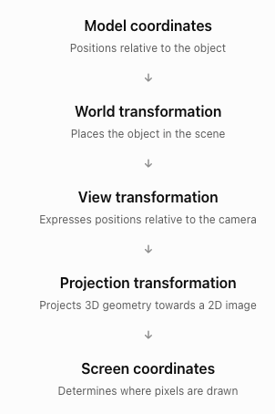
Using column vectors, a typical transformation pipeline is:
where:
-
M is the model matrix.
-
V is the view matrix.
-
P_proj is the projection matrix.
-
P_model is the original point in homogeneous coordinates.
The result is in clip coordinates. For perspective projection, the computer subsequently performs a perspective division and viewport mapping to obtain screen coordinates.
Orthographic and Perspective Projection
Orthographic projection
Parallel lines remain parallel, and distant objects do not appear smaller simply because of their distance.
Perspective projection
Objects farther from the camera appear smaller, producing a more realistic sense of depth.
These projection methods are used in computer-aided design, architectural drawings, video games, and animation.
Analysing Graphical Transformations Using Determinants
The determinant of a transformation matrix reveals useful geometric information.
For a 2 × 2 matrix A:
The sign of the determinant indicates whether orientation is preserved or reversed.
|
Determinant |
Interpretation |
|---|---|
|
det(A) > 0 |
Orientation preserved |
|
det(A) < 0 |
Orientation reversed |
|
det(A) = 0 |
Area collapses to zero |
|
|det(A)| = 1 |
Area preserved |
|
|det(A)| > 1 |
Area enlarged |
|
0 < |det(A)| < 1 |
Area reduced |
Worked Example 12: Analysing a Transformation
Consider:
Calculate:
det(A) = 2(3) − 1(0)
= 6
Therefore:
-
Areas are multiplied by 6.
-
Orientation is preserved.
-
The transformation is invertible.
If a shape originally has an area of 5 cm², its transformed area is:
5 × 6 = 30 cm²
This provides a useful way to check whether a graphical transformation behaves as expected.
Real-World Applications in Technology
Video Games and Animation
Matrices control the positions, rotations, and sizes of characters, objects, cameras, and virtual environments. A character's limbs can be positioned using linked transformations, similar to a robotic arm.
Augmented Reality
Virtual objects are positioned relative to the real environment using transformations that account for the camera's position and orientation.
Medical Robotics
Robotic surgical systems use coordinate transformations to help position instruments accurately. Sensor measurements and control systems provide additional information needed for safe movement.
Autonomous Vehicles and Robots
Robots combine coordinate transformations with sensor data to estimate positions, construct maps, detect obstacles, and plan movement.
Computer-Aided Design
Engineers use transformations to position components, construct assemblies, examine designs, and visualise objects from different viewpoints.
Evaluating Matrix-Based Models
Matrix models are powerful, but real-world graphics and robotics involve additional complexities.
Numerical Accuracy
Computers usually store decimal values with limited precision.
Repeated transformations can introduce small rounding errors.
For example, repeatedly rotating an object through many small angles may eventually produce a slight numerical difference from the expected position.
Physical Constraints
A mathematical transformation may describe a position that a robot cannot physically reach.
Robots have:
-
Limited joint rotation.
-
Maximum extension lengths.
-
Motor speed limits.
-
Load restrictions.
-
Collision constraints.
Coordinate Conventions
Different graphics and robotics systems may use different conventions.
These include:
-
Left-handed or right-handed coordinate systems.
-
Row vectors or column vectors.
-
Different axis orientations.
-
Different rotation orders.
-
Degrees or radians.
A transformation must be interpreted using the conventions of the system.
Model Validation
Engineers verify transformations by checking:
-
Whether calculated positions agree with measured positions.
-
Whether distances and angles are preserved when expected.
-
Whether the transformation matrix is valid.
-
Whether movement remains within physical limits.
-
Whether numerical errors are acceptably small.
Common Mistakes
Mistake 1: Multiplying transformation matrices in the wrong order
Matrix multiplication is generally not commutative. Rotation followed by scaling may produce a different result from scaling followed by rotation.
Mistake 2: Confusing clockwise and counterclockwise rotations
The standard 2D rotation matrix uses positive angles for counterclockwise rotation.
Mistake 3: Forgetting that a 2 × 2 matrix cannot represent a nonzero translation
Use homogeneous coordinates and a 3 × 3 matrix for 2D translation.
Mistake 4: Confusing horizontal and vertical scaling factors
The first diagonal entry scales x, while the second scales y.
Mistake 5: Assuming all transformations preserve distances
Rotations and reflections preserve distances, but general scaling and shearing do not.
Mistake 6: Ignoring the centre of rotation
A standard rotation matrix rotates about the origin. Rotation about another point requires translations as well.
Mistake 7: Confusing local and global coordinates
A robot joint's local coordinates may differ from coordinates measured relative to the robot's base.
Mistake 8: Treating the second robot joint angle as an absolute angle
In a standard two-link robotic arm, θ₂ is measured relative to the first link, so the second link's absolute orientation is θ₁ + θ₂.
Mistake 9: Assuming every target position is reachable
A robot's link lengths and joint limits restrict its workspace.
Mistake 10: Forgetting to check matrix dimensions
A transformation matrix must have compatible dimensions with the vector or matrix it transforms.
Mistake 11: Misinterpreting determinants
The absolute determinant gives area scaling in 2D, while the sign indicates orientation.
Mistake 12: Confusing a model with physical reality
Robotic movement also depends on motors, sensors, forces, and environmental conditions.
Key Terms
-
Computer Graphics: Creation and manipulation of visual images using computers.
-
Vertex: Point defining part of a geometric object.
-
Transformation Matrix: Matrix used to change coordinates or geometric properties.
-
Translation: Movement of an object by a fixed displacement.
-
Rotation: Turning an object around a point or axis.
-
Reflection: Flipping an object across a line or plane.
-
Scaling: Changing the size of an object.
-
Uniform Scaling: Scaling by the same factor in every direction.
-
Non-Uniform Scaling: Scaling by different factors in different directions.
-
Shear: Transformation that slants an object.
-
Homogeneous Coordinates: Extended coordinate representation that allows translations to be combined with linear transformations using matrices.
-
Affine Transformation: Transformation combining linear operations and translation.
-
Composite Transformation: Combination of multiple transformations.
-
Rotation Matrix: Matrix representing rotation through a specified angle.
-
Determinant: Scalar describing geometric scaling and orientation properties.
-
Orientation: Directional alignment of an object or coordinate frame.
-
Coordinate Frame: Reference system used to describe positions and orientations.
-
World Coordinates: Coordinates relative to a fixed global reference.
-
Local Coordinates: Coordinates relative to an object or component.
-
End Effector: Working tool or terminal component of a robot.
-
Joint Angle: Angle describing the rotation of a robotic joint.
-
Forward Kinematics: Calculation of tool position and orientation from joint variables.
-
Inverse Kinematics: Calculation of joint variables needed to reach a desired position or orientation.
-
Workspace: Region a robot can reach.
-
Transformation Pipeline: Sequence of coordinate transformations used in graphics.
-
View Matrix: Matrix expressing coordinates relative to a camera.
-
Projection Matrix: Matrix used to project 3D geometry for display.
-
Orthographic Projection: Projection without perspective size reduction.
-
Perspective Projection: Projection in which distant objects appear smaller.
-
Computer Vision: Field involving the interpretation of images and visual data.
-
Robotic Manipulator: Robot designed to position and move objects or tools.
Key Takeaways
-
Computer graphics uses matrices to represent and transform objects.
-
Vertices can be organised into matrices so many points can be transformed simultaneously.
-
Rotation, reflection, scaling, and shear can be represented using 2 × 2 matrices in two dimensions.
-
Homogeneous coordinates allow translation to be represented using matrix multiplication.
-
Composite transformations are calculated by multiplying matrices in the correct order.
-
Transformation order can change the final result.
-
Three-dimensional graphics uses matrices to rotate and position objects in space.
-
Robotics uses transformation matrices to describe positions and orientations of robot components.
-
Forward kinematics calculates tool positions from joint angles.
-
Inverse kinematics calculates joint angles needed to reach target positions.
-
Determinants reveal geometric scaling and orientation.
-
Coordinate transformations are essential in animation, computer-aided design, autonomous systems, and robotics.
-
Mathematical results must be checked against physical constraints and real-world measurements.
Check Your Understanding
Questions
Question 1: Computer Graphics
Explain why matrices are useful when transforming objects containing many vertices.
Question 2: Rotation
Rotate P = (4, 2) by 90° counterclockwise about the origin.
Question 3: Reflection
Reflect P = (−3, 5) in the x-axis.
Question 4: Scaling
Scale P = (2, −4) horizontally by factor 3 and vertically by factor 0.5.
Question 5: Shear
Apply a horizontal shear with k = 2 to P = (3, 2).
Question 6: Transformation Order
A point P = (1, 2) is rotated 90° counterclockwise, then scaled uniformly by factor 3.
Find the final coordinates.
Question 7: Homogeneous Translation
Translate P = (−2, 5) by 4 units right and 3 units down using a homogeneous transformation matrix.
Question 8: Combined Transformation
A point P = (2, 1) is rotated 90° counterclockwise and then translated 3 units right.
Construct the combined homogeneous transformation matrix and find P′.
Question 9: Three-Dimensional Rotation
Rotate P = (1, 3, 2) by 90° about the z-axis.
Question 10: Determinants
A transformation matrix is:
Determine the area scale factor.
Question 11: Robotic Arm
A two-link robotic arm has:
L₁ = 5 m
L₂ = 3 m
θ₁ = 0°
θ₂ = 90°
Calculate the end effector's position.
Question 12: Reachability
A robotic arm has segment lengths 6 m and 4 m.
Assuming unrestricted planar revolute joints, determine its minimum and maximum reachable distances from the base.
Question 13: Forward and Inverse Kinematics
Explain the difference between forward kinematics and inverse kinematics.
Question 14: Technology Applications
Describe two practical applications of transformation matrices in technology.
Question 15: Integrated Challenge
A triangle has vertices:
A = (1, 1)
B = (3, 1)
C = (2, 4)
The triangle undergoes the following transformations:
-
A 90° counterclockwise rotation about the origin.
-
A horizontal enlargement by factor 2.
-
A translation 4 units right and 1 unit up.
a) Write the rotation matrix.
b) Write the scaling matrix.
c) Construct the combined 3 × 3 homogeneous transformation matrix.
d) Calculate the final coordinates of all three vertices.
e) Calculate the determinant of the linear part of the transformation.
f) Determine the area scale factor.
g) Explain whether the transformation preserves orientation.
Fully Worked Answers
Answer 1: Computer Graphics
Matrices allow the same transformation to be applied systematically to many vertices.
If V contains the coordinates of an object and T is a transformation matrix:
V′ = TV
This allows an entire object to be rotated, reflected, scaled, or sheared using matrix multiplication.
Answer 2: Rotation
Answer 3: Reflection
Reflection in the x-axis:
(x, y) → (x, −y)
Therefore:
Answer 4: Scaling
Answer 5: Shear
Horizontal shear:
x′ = 3 + 2(2) = 7
y′ = 2
Answer 6: Transformation Order
Start:
P = (1, 2)
Rotate 90° counterclockwise:
(1, 2) → (−2, 1)
Scale uniformly by factor 3:
(−2, 1) → (−6, 3)
Answer 7: Homogeneous Translation
The translation is:
a = 4
b = −3
Therefore:
Apply to:
Answer 8: Combined Transformation
Rotation matrix in homogeneous coordinates:
Translation matrix:
Combined matrix:
Apply to P = (2, 1):
Answer 9: Three-Dimensional Rotation
For a 90° rotation about the z-axis:
(x, y, z) → (−y, x, z)
Therefore:
(1, 3, 2) → (−3, 1, 2)
Answer 10: Determinants
Calculate:
det(A) = 3(2) − 0
= 6
Therefore:
Areas become six times as large.
Answer 11: Robotic Arm
Given:
L₁ = 5
L₂ = 3
θ₁ = 0°
θ₂ = 90°
Horizontal position:
x = 5 cos 0° + 3 cos 90°
x = 5(1) + 3(0)
x = 5
Vertical position:
y = 5 sin 0° + 3 sin 90°
y = 5(0) + 3(1)
y = 3
Answer 12: Reachability
Maximum reach:
L₁ + L₂ = 6 + 4 = 10 m
Minimum reach:
|L₁ − L₂| = |6 − 4| = 2 m
Therefore:
The arm can reach points whose distance from the base lies between 2 m and 10 m, assuming no joint limits or obstacles.
Answer 13: Forward and Inverse Kinematics
Forward kinematics calculates the end effector's position and orientation from known joint angles and link lengths.
Inverse kinematics calculates the joint angles required to reach a desired position or orientation.
Forward kinematics usually gives a direct calculation.
Inverse kinematics may have multiple solutions, one solution, or no solution.
Answer 14: Technology Applications
Application 1: Video Games
Transformation matrices move, rotate, and scale game objects and characters.
Application 2: Industrial Robotics
Transformation matrices calculate the positions and orientations of robotic arms, grippers, and tools.
Other valid examples include computer-aided design, augmented reality, medical robotics, and autonomous navigation.
Answer 15: Integrated Challenge
Original vertices:
A = (1, 1)
B = (3, 1)
C = (2, 4)
Part a: Rotation matrix
Part b: Scaling matrix
Horizontal enlargement by factor 2:
Part c: Combined homogeneous matrix
First rotate, then scale, then translate.
Homogeneous rotation:
Homogeneous scaling:
Translation:
The combined transformation is:
First:
Then:
Part d: Final coordinates
For A = (1, 1):
x′ = −2 + 4 = 2
y′ = 1 + 1 = 2
A′ = (2, 2)
For B = (3, 1):
x′ = −2 + 4 = 2
y′ = 3 + 1 = 4
B′ = (2, 4)
For C = (2, 4):
x′ = −8 + 4 = −4
y′ = 2 + 1 = 3
C′ = (−4, 3)
Therefore:
Part e: Determinant
The linear part is:
Calculate:
det(A) = 0(0) − (−2)(1)
Part f: Area scale factor
The area scale factor is:
|det(A)| = 2
Therefore, the transformed triangle has twice the original area.
As an additional check, the original triangle has base 2 and height 3:
Area = 1/2 × 2 × 3 = 3 square units
The transformed area is:
2 × 3 = 6 square units
Part g: Orientation
Since:
det(A) = 2 > 0
the transformation preserves orientation.
The rotation preserves orientation, the positive scaling preserves orientation, and translation does not change orientation.
Final Reflection
Matrices provide a common mathematical language for computer graphics and robotics.
In computer graphics, transformation matrices allow objects to be rotated, reflected, scaled, sheared, and translated. Homogeneous coordinates make it possible to combine these operations into a single matrix, while three-dimensional transformations allow virtual objects to be positioned and displayed from different viewpoints.
In robotics, matrices describe the positions and orientations of moving components. Forward kinematics allows engineers to calculate where a robot's tool will move, while inverse kinematics helps determine how joints must move to reach a target.
The same mathematical principles therefore connect animated characters, virtual environments, industrial machinery, autonomous vehicles, and medical robots.
The central idea is that matrices provide an efficient, systematic way to describe and combine movements in both virtual and physical space.
5. Applications in Science and Engineering
Learning outcomes
- I can apply matrices to engineering problems.
- I can model physical systems using matrices.
- I can analyse scientific data with matrices.
- I can interpret mathematical models.
- I can solve authentic STEM applications.
Introduction
Matrices are among the most useful mathematical tools in science and engineering. They allow scientists and engineers to organise large amounts of information, describe relationships between variables, solve simultaneous equations, and predict how physical systems will behave.
Consider some important questions:
-
How can engineers calculate the forces acting on a bridge?
-
How can electrical engineers determine currents in a complicated circuit?
-
How can scientists analyse measurements from several experiments?
-
How can engineers predict the movement of a mechanical system?
-
How can environmental scientists model the movement of pollutants?
-
How can researchers use data to identify relationships between physical quantities?
Although these problems involve different scientific disciplines, many can be represented using the same mathematical structure:
where:
-
A is a matrix containing the relationships between variables.
-
x is a vector containing unknown quantities.
-
b is a vector containing known values.
Once a problem has been represented using matrices, mathematical methods can be used to calculate unknown quantities, analyse relationships, and evaluate possible solutions.
In this lesson, we will explore how matrices are applied to engineering systems, mechanics, electrical circuits, scientific data, population models, and other authentic STEM problems.
Why Matrices Are Important in STEM
Scientific and engineering problems often involve several variables that interact with one another.
For example, the movement of an object may depend on:
-
Position
-
Velocity
-
Acceleration
-
Applied forces
-
Mass
-
Time
An electrical circuit may involve:
-
Voltage
-
Current
-
Resistance
-
Multiple branches
-
Several connected components
A matrix provides an organised way to represent these relationships.
The General Matrix Model
Consider the simultaneous equations:
2x + 3y = 12
4x − y = 5
These can be written as:
Or:
The coefficient matrix is:
The unknown vector is:
The known vector is:
If A is invertible:
For larger systems, engineers usually use numerical methods such as matrix factorisation rather than calculating the inverse explicitly.
Worked Example 1: Solving an Engineering System
Solve:
3x + 2y = 16
x + 4y = 12
Write the matrix equation:
Calculate the determinant:
det(A) = 3(4) − 2(1) = 10
The inverse is:
Therefore:
Therefore:
Verify:
3(4) + 2(2) = 16
4 + 4(2) = 12
Both equations are satisfied.
Matrices in Structural Engineering
Structural engineers analyse buildings, bridges, towers, and other structures to ensure they can support applied forces.
Forces may include:
-
The weight of the structure.
-
The weight of people and vehicles.
-
Wind loads.
-
Earthquake forces.
-
Tension and compression in structural members.
A structure must satisfy the conditions of equilibrium.
For a stationary object in two dimensions:
For a rigid body, rotational equilibrium is also required:
These equations can be combined into matrix form.
Worked Example 2: Forces in Two Supporting Cables
A 100 N load is supported by two cables.
Cable A makes an angle of 30° above the horizontal.
Cable B makes an angle of 60° above the horizontal on the opposite side.
Find the tension in each cable.
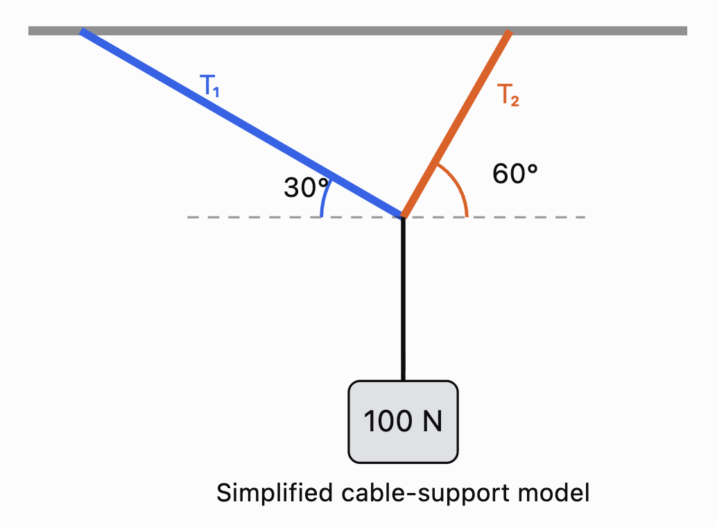
Let:
T₁ = tension in Cable A
T₂ = tension in Cable B
Step 1: Horizontal Equilibrium
The horizontal forces must balance.
Rearrange:
Step 2: Vertical Equilibrium
The upward forces must equal the weight.
Step 3: Write the Matrix Equation
Substitute approximate trigonometric values:
Step 4: Solve
From the horizontal equation:
0.866T₁ = 0.5T₂
Therefore:
T₂ ≈ 1.732T₁
Substitute into the vertical equation:
0.5T₁ + 0.866(1.732T₁) = 100
0.5T₁ + 1.5T₁ = 100
2T₁ = 100
T₁ = 50 N
Then:
T₂ ≈ 1.732(50)
T₂ ≈ 86.6 N
Therefore:
Interpretation
The cable at 60° has the greater tension.
The two cables together provide sufficient upward force to support the 100 N load while their horizontal components cancel.
Matrix methods become particularly valuable when a structure contains many connected members and unknown forces.
Matrices in Electrical Engineering
Electrical engineers use matrices to analyse circuits containing multiple resistors, voltage sources, and branches.
Two important principles are:
Ohm's Law
where:
-
V = voltage (V)
-
I = current (A)
-
R = resistance (Ω)
Kirchhoff's Voltage Law
The algebraic sum of voltage changes around a closed loop is zero.
Kirchhoff's Current Law states that the total current entering a junction equals the total current leaving it.
These laws produce systems of linear equations that can be solved using matrices.
Worked Example 3: A Two-Loop Circuit
Consider two adjacent circuit loops sharing a resistor.
Suppose the mesh-current equations obtained from Kirchhoff's laws are:
5I₁ − 2I₂ = 12
−2I₁ + 6I₂ = 6
Here, the coefficients represent resistances in ohms and the constants represent voltages.
Write the system as:
Step 1: Calculate the Determinant
det(A) = 5(6) − (−2)(−2)
= 30 − 4
= 26
Step 2: Calculate the Inverse
Step 3: Solve for the Currents
Therefore:
Interpretation
The two mesh currents are approximately 3.23 A and 2.08 A.
If the mesh currents pass through the shared resistor in opposite directions, the current through that resistor is:
I₁ − I₂ ≈ 1.15 A
The matrix method provides an organised way to calculate multiple currents simultaneously.
Matrices in Mechanical Engineering
Mechanical engineers use matrices to model systems involving forces, motion, deformation, and vibration.
A common example is a system of masses connected by springs.
Hooke's Law
For an ideal spring:
where:
-
F = restoring force
-
k = spring constant
-
x = displacement from equilibrium
The negative sign indicates that the restoring force acts opposite to the displacement.
Coupled Spring Systems
Suppose two movable masses are connected to fixed walls and to each other by springs.
Let:
x₁ = displacement of Mass 1
x₂ = displacement of Mass 2
If the system is displaced slightly from equilibrium, the restoring-force equations can be written:
In matrix form:
where:
and:
M is called the mass matrix.
K is called the stiffness matrix.
This matrix equation describes how the masses move together.
It is important in the study of:
-
Vehicle suspension systems.
-
Building vibrations.
-
Earthquake engineering.
-
Mechanical resonance.
-
Aircraft structures.
-
Industrial machinery.
Worked Example 4: Static Spring Displacements
Consider a simplified spring system whose static equilibrium is described by:
The stiffness coefficients are measured in N/m, the applied forces in N, and the displacements in m.
This gives:
30x₁ − 10x₂ = 50
−10x₁ + 20x₂ = 20
Divide both equations by 10:
3x₁ − x₂ = 5
−x₁ + 2x₂ = 2
From the first equation:
x₂ = 3x₁ − 5
Substitute into the second:
−x₁ + 2(3x₁ − 5) = 2
−x₁ + 6x₁ − 10 = 2
5x₁ = 12
x₁ = 2.4
Then:
x₂ = 3(2.4) − 5
x₂ = 2.2
Therefore:
These are the displacements predicted by the ideal linear spring model.
In a real engineering application, such large displacements might exceed the range where Hooke's law is valid. Engineers would need to check whether the model's assumptions remain reasonable.
Matrices in Scientific Data Analysis
Scientists frequently collect measurements from experiments.
Matrices allow data to be organised and analysed efficiently.
Suppose an experiment measures the temperature and pressure of a gas at several times.
|
Trial |
Temperature (K) |
Pressure (kPa) |
|---|---|---|
|
1 |
300 |
100 |
|
2 |
320 |
107 |
|
3 |
340 |
113 |
|
4 |
360 |
120 |
The data can be represented by:
Each row represents an observation.
Each column represents a measured variable.
Matrices are particularly useful when datasets contain many observations and several variables.
Data Transformations
Suppose all temperatures must be converted from kelvin to degrees Celsius.
The conversion is:
°C = K − 273.15
The temperature column can be transformed by subtracting 273.15 from each entry.
More generally, data can be transformed using matrix operations to:
-
Change units.
-
Centre variables around their means.
-
Standardise measurements.
-
Combine datasets.
-
Calculate predictions.
-
Identify patterns.
Matrices and Linear Regression
One of the most important applications of matrices in scientific data analysis is linear regression.
Linear regression finds a mathematical relationship between variables.
Suppose we believe the relationship between two quantities is approximately linear:
where:
-
m = gradient
-
c = intercept
If several measurements are available, we can construct a matrix equation.
For observations (x₁, y₁), (x₂, y₂), ..., (xₙ, yₙ):
The unknown parameter vector is:
The observed values are:
We model:
The least-squares solution minimises the sum of squared residuals.
When X has full column rank:
This formula is called the normal-equation solution.
For numerical work, QR factorisation or other stable methods are often preferred over explicitly forming the inverse.
Worked Example 5: Finding a Line of Best Fit
A student measures the extension of a spring under different forces.
|
Force x (N) |
Extension y (cm) |
|---|---|
|
1 |
2 |
|
2 |
4 |
|
3 |
5 |
We want to model:
y = mx + c
Construct:
and:
Calculate:
Also:
The normal equations are:
This gives:
14m + 6c = 25
6m + 3c = 11
Multiply the second equation by 2:
12m + 6c = 22
Subtract:
2m = 3
m = 1.5
Substitute:
6(1.5) + 3c = 11
9 + 3c = 11
c = 2/3
Therefore:
The model predicts an extension of approximately 1.5 cm for every additional newton of force, with an intercept of approximately 0.667 cm.
In a perfectly calibrated Hooke's law experiment, extension would be expected to be zero at zero applied force. The nonzero intercept may reflect measurement error, a zero offset, or limitations in the data.
Visualising Scientific Regression
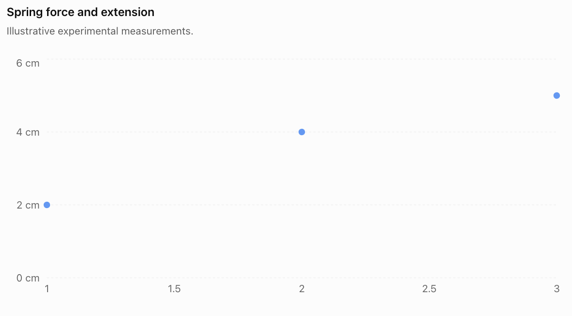
The matrix regression model allows scientists to estimate a relationship even when measurements do not lie exactly on a straight line.
This is useful because real experimental data almost always contains uncertainty.
Matrices in Population and Environmental Science
Matrices can also model how populations change over time.
Suppose a population contains two age groups:
-
Juveniles
-
Adults
The number of individuals in each group can be represented by a population vector:
where:
-
Jₙ = number of juveniles at time n.
-
Aₙ = number of adults at time n.
A transition matrix describes survival, reproduction, and movement between age groups.
Worked Example 6: Population Growth
Suppose:
-
Each adult produces an average of 2 juveniles per year.
-
50% of juveniles survive to become adults.
-
80% of adults survive into the following year.
-
Juveniles do not remain in the juvenile category after one year.
The population matrix is:
Initially, there are:
100 juveniles
50 adults
Therefore:
The next year's population is:
Juveniles:
0(100) + 2(50) = 100
Adults:
0.5(100) + 0.8(50) = 90
Therefore:
After one year, the model predicts:
-
100 juveniles
-
90 adults
Total population = 190
Predicting the Second Year
Juveniles:
0(100) + 2(90) = 180
Adults:
0.5(100) + 0.8(90) = 122
Therefore:
Total population = 302
Interpretation
The model predicts population growth.
However, this does not guarantee that the real population will continue increasing indefinitely.
The model assumes constant reproduction and survival rates and does not account for limited food, disease, competition, or environmental changes.
Notice that this is not a probability transition matrix: the first column and second column do not both sum to 1. Reproduction can add new individuals, so total population is not necessarily conserved.
Matrices in Chemical Engineering
Chemical engineers use matrices to model chemical reactions, material flows, and industrial production processes.
One important application is balancing chemical equations.
Representing Chemical Reactions with Matrices
Consider the combustion of methane:
CH₄ + O₂ → CO₂ + H₂O
Let the unknown coefficients be:
aCH₄ + bO₂ → cCO₂ + dH₂O
Conservation of atoms gives three equations.
Carbon:
a − c = 0
Hydrogen:
4a − 2d = 0
Oxygen:
2b − 2c − d = 0
These can be represented as:
This is a homogeneous system of linear equations.
Worked Example 7: Balancing a Chemical Equation
From carbon conservation:
a = c
From hydrogen conservation:
4a = 2d
Therefore:
d = 2a
From oxygen conservation:
2b = 2c + d
Substitute c = a and d = 2a:
2b = 2a + 2a
2b = 4a
b = 2a
Choose the smallest positive integer value:
a = 1
Then:
b = 2
c = 1
d = 2
Therefore:
Why Matrices Are Useful
For simple chemical reactions, balancing by inspection is often faster.
However, complicated chemical reactions may contain many elements and compounds.
Matrix methods allow the conservation equations to be organised and solved systematically.
This is especially useful in chemical engineering software and reaction-network modelling.
Matrices in Computer Science and Engineering
Matrices are used extensively in computing, particularly in graphics, machine learning, image processing, and robotics.
A digital image can be represented as a matrix of pixel values.
For a grayscale image, each matrix entry represents the brightness of a pixel.
For example:
Here, pixel values range from 0 to 255.
-
0 represents black.
-
255 represents white.
-
Intermediate values represent shades of gray.

Matrix operations can be used to:
-
Increase or decrease brightness.
-
Rotate and resize images.
-
Detect edges.
-
Reduce noise.
-
Apply filters.
-
Analyse image patterns.
Worked Example 8: Increasing Image Brightness
Suppose an image has pixel matrix:
\[ I=\begin{bmatrix} 50&100\\ 150&200 \end{bmatrix} \]We want to increase every pixel value by 30.
Add:
\[ B=\begin{bmatrix} 30&30\\ 30&30 \end{bmatrix} \]Then:
\[ I'=I+B \]\[ I'= \begin{bmatrix} 80&130\\ 180&230 \end{bmatrix} \]Therefore:
\[ \boxed{ I'=\begin{bmatrix} 80&130\\ 180&230 \end{bmatrix} } \]The image becomes brighter.
If a calculation produces a value above 255, an 8-bit image-processing system must handle the value appropriately, often by clipping it to 255.
Matrices in Fluid Flow and Environmental Modelling
Environmental scientists and engineers use matrices to model the movement of water, air, pollutants, and other substances.
Suppose a lake is divided into two regions.
Each day:
-
80% of the pollutant in Region A remains there.
-
20% moves from A to B.
-
10% of the pollutant in Region B moves to A.
-
90% remains in B.
The transition matrix is:
\[ T=\begin{bmatrix} 0.8&0.1\\ 0.2&0.9 \end{bmatrix} \]Suppose initially:
Region A contains 100 kg of pollutant.
Region B contains 50 kg.
Then:
\[ \mathbf{P}_0=\begin{bmatrix}100\\50\end{bmatrix} \]Worked Example 9: Pollutant Movement
Calculate:
\[ \mathbf{P}_1=T\mathbf{P}_0 \]\[ \mathbf{P}_1= \begin{bmatrix} 0.8&0.1\\ 0.2&0.9 \end{bmatrix} \begin{bmatrix} 100\\50 \end{bmatrix} \]Region A:
0.8(100) + 0.1(50)
= 80 + 5
= 85 kg
Region B:
0.2(100) + 0.9(50)
= 20 + 45
= 65 kg
Therefore:
\[ \boxed{\mathbf{P}_1=\begin{bmatrix}85\\65\end{bmatrix}\text{ kg}} \]The total remains:
85 + 65 = 150 kg
This is consistent with the model's assumption that pollutant moves between regions but is not created or destroyed.
Model Limitations
The model does not include:
-
Chemical decomposition.
-
Evaporation.
-
New pollution sources.
-
Changes in water flow.
-
Seasonal weather patterns.
-
Pollutant absorption by sediments or organisms.
A more advanced model could include additional regions and processes.
Analysing and Interpreting Matrix Models
A mathematical model is useful only when its results can be interpreted meaningfully.
Scientists and engineers must consider several important questions.
Are the Units Consistent?
Suppose a stiffness matrix is measured in N/m and a displacement vector is measured in m.
Then:
\[ K\mathbf{x}=\mathbf{F} \]The units are:
(N/m) × m = N
This produces a force vector, as expected.
Dimensional analysis helps identify errors in scientific models.
Does the Solution Make Physical Sense?
A mathematical solution may be correct but physically impossible.
Examples include:
-
A negative mass.
-
A probability greater than 1.
-
A robotic arm reaching beyond its maximum length.
-
A structural member carrying a force beyond its safe capacity.
-
A predicted temperature outside the model's valid range.
Solutions must be checked against physical constraints.
Is the Model Sensitive to Changes?
A model may be highly sensitive to small changes in its inputs.
For example, a small measurement error may produce a large change in the calculated solution if the coefficient matrix is nearly singular.
The condition number of a matrix is one measure of this sensitivity.
A large condition number indicates that small errors in the data may cause relatively large errors in the calculated solution.
Is the Model Appropriate?
A linear matrix model may work well for small changes but fail for larger changes.
For example:
-
Springs may stop obeying Hooke's law.
-
Air resistance may depend nonlinearly on speed.
-
Population growth may be limited by resources.
-
Material properties may change with temperature.
Scientists must choose models appropriate to the situation.
Sensitivity Analysis: An Engineering Example
Consider the system:
\[ \begin{bmatrix} 1&1\\ 1&1.01 \end{bmatrix} \begin{bmatrix} x\\y \end{bmatrix} = \begin{bmatrix} 2\\2.01 \end{bmatrix} \]The equations are:
x + y = 2
x + 1.01y = 2.01
Subtract the first equation from the second:
0.01y = 0.01
y = 1
Therefore:
x = 1
The solution is:
\[ \boxed{(x,y)=(1,1)} \]Now suppose the second measured value changes slightly from 2.01 to 2.02.
The new system is:
x + y = 2
x + 1.01y = 2.02
Subtract:
0.01y = 0.02
y = 2
Then:
x = 0
The new solution is:
\[ \boxed{(x,y)=(0,2)} \]A change of only 0.01 in the measured value produced a large change in the solution.
This happens because the equations are nearly dependent.
The example demonstrates why scientists and engineers must consider measurement uncertainty and numerical sensitivity.
Choosing the Correct Matrix Method
Different STEM problems require different matrix techniques.
Problem
Matrix technique
Simultaneous engineering equations
Gaussian elimination or matrix factorisation
Small invertible linear systems
Inverse matrix
Structural force calculations
Equilibrium equations in matrix form
Electrical circuits
Kirchhoff's laws and linear systems
Spring and vibration systems
Mass and stiffness matrices
Scientific regression
Least squares
Population growth
Matrix recurrence models
Chemical equation balancing
Null space of a matrix
Image processing
Matrix and array operations
Environmental transport
Transition and flow matrices
Stability of dynamic systems
Eigenvalues and eigenvectors
The appropriate method depends on the mathematical structure of the problem.
A key skill in applied mathematics is recognising which matrix method best represents the situation.
Common Mistakes
Mistake 1: Constructing the matrix incorrectly
Rows and columns must represent the intended variables and relationships. Incorrect placement of coefficients produces incorrect results.
Mistake 2: Ignoring the order of matrix multiplication
In general, AB ≠ BA. The order must reflect the physical or mathematical process.
Mistake 3: Forgetting units
A numerical answer without appropriate units may be meaningless in an engineering context.
Mistake 4: Assuming every matrix has an inverse
A matrix must be square and nonsingular to have an inverse.
Mistake 5: Using an inverse when a more suitable method is available
Large engineering systems are generally solved using numerical factorisation methods rather than explicitly calculating inverse matrices.
Mistake 6: Confusing a population matrix with a probability transition matrix
A population matrix may include reproduction and growth. Its columns do not necessarily sum to 1.
Mistake 7: Assuming experimental measurements are exact
Real scientific data contains measurement uncertainty and possible systematic errors.
Mistake 8: Confusing correlation with causation
A relationship identified using matrix regression does not automatically establish that one variable causes another.
Mistake 9: Ignoring physical constraints
A mathematical solution may violate real-world limits such as material strength, capacity, or conservation laws.
Mistake 10: Treating model predictions as guaranteed outcomes
Models depend on assumptions and available data. Predictions should be interpreted as estimates.
Mistake 11: Ignoring numerical sensitivity
Nearly singular matrices can produce solutions that are highly sensitive to small measurement errors.
Mistake 12: Failing to verify results
Solutions should be substituted into the original equations and checked against the physical situation.
Key Terms
-
Mathematical Model: Mathematical representation of a real-world system.
-
Coefficient Matrix: Matrix containing the coefficients of a system of equations.
-
Variable Vector: Column vector containing unknown quantities.
-
Inverse Matrix: Matrix that reverses the effect of an invertible matrix.
-
Singular Matrix: Square matrix with determinant zero.
-
Gaussian Elimination: Method of solving linear systems using row operations.
-
Matrix Factorisation: Representation of a matrix as a product of simpler matrices.
-
Equilibrium: Condition in which net force and net torque are zero.
-
Tension: Pulling force transmitted through a cable or similar component.
-
Kirchhoff's Voltage Law: Principle that the algebraic sum of voltage changes around a closed loop is zero.
-
Kirchhoff's Current Law: Principle that total current entering a junction equals total current leaving.
-
Mesh Current: Assigned circulating current used to analyse a circuit loop.
-
Hooke's Law: Relationship between restoring force and displacement for an ideal spring.
-
Stiffness Matrix: Matrix relating displacements to forces in a linear mechanical system.
-
Mass Matrix: Matrix representing the mass properties of a mechanical system.
-
Linear Regression: Method for modelling a linear relationship between variables.
-
Least Squares: Method that minimises the sum of squared residuals.
-
Residual: Difference between an observed value and a predicted value.
-
Normal Equations: Matrix equations used to obtain a least-squares solution.
-
Population Matrix: Matrix describing survival, reproduction, or movement between population groups.
-
Homogeneous System: Linear system of the form Ax = 0.
-
Null Space: Set of vectors mapped to zero by a matrix.
-
Transition Matrix: Matrix describing changes between states.
-
Pixel Matrix: Array of numerical values representing image pixels.
-
Eigenvalue: Scalar describing how an eigenvector is scaled by a matrix.
-
Condition Number: Measure of sensitivity to errors in inputs or calculations.
-
Dimensional Analysis: Checking relationships using physical units.
-
Model Validation: Comparing model predictions with observed evidence.
-
Sensitivity Analysis: Investigating how changes in inputs affect outputs.
-
Conservation Law: Scientific principle stating that a quantity is conserved under specified conditions.
Key Takeaways
-
Matrices provide an organised way to represent complex scientific and engineering systems.
-
Many STEM problems can be expressed as Ax = b.
-
Structural engineers use matrices to calculate forces and support loads.
-
Electrical engineers use matrices to solve circuit equations.
-
Mechanical engineers use mass and stiffness matrices to model motion and vibration.
-
Scientific datasets can be organised into matrices for analysis.
-
Matrix least-squares methods help determine relationships between measured variables.
-
Population matrices can model survival, reproduction, and population growth.
-
Chemical equations can be balanced using homogeneous linear systems.
-
Images can be represented and processed using matrices of pixel values.
-
Transition matrices can model the movement of pollutants between regions.
-
Eigenvalues can help analyse the stability and behaviour of physical systems.
-
Nearly singular matrices can produce solutions sensitive to measurement errors.
-
Scientific models must be interpreted using correct units, physical constraints, and realistic assumptions.
Check Your Understanding
Questions
Question 1: Matrix Representation
Represent the following system in matrix form:
3x + 2y = 14
5x − y = 8
Question 2: Engineering Equations
Solve the system from Question 1.
Question 3: Structural Engineering
A load is supported by two vertical cables carrying tensions T₁ and T₂.
The total upward force is 200 N.
Cable 1 carries 40 N more tension than Cable 2.
Construct a matrix equation and calculate both tensions.
Question 4: Electrical Engineering
Two mesh currents satisfy:
4I₁ − I₂ = 11
−I₁ + 3I₂ = 7
Calculate I₁ and I₂.
Question 5: Spring Systems
A mechanical system is represented by:
\[ \begin{bmatrix} 20&-5\\ -5&15 \end{bmatrix} \begin{bmatrix} x_1\\x_2 \end{bmatrix} = \begin{bmatrix} 35\\25 \end{bmatrix} \]Calculate the two displacements. Assume stiffness coefficients are in N/m and forces in N.
Question 6: Scientific Data
A scientist records the following measurements:
Time (s)
Distance (m)
1
3
2
6
3
9
Represent the measurements using a 3 × 2 data matrix.
Question 7: Linear Regression
The points (1, 2), (2, 4), and (3, 6) lie on a straight line.
Determine the regression equation y = mx + c.
Question 8: Population Modelling
A population is modelled by:
\[ L=\begin{bmatrix} 0&3\\ 0.4&0.7 \end{bmatrix} \]Initially:
\[ \mathbf{P}_0=\begin{bmatrix} 50\\40 \end{bmatrix} \]Calculate the population after one year.
Question 9: Chemical Engineering
Balance the chemical equation using conservation of atoms:
Fe + O₂ → Fe₂O₃
Question 10: Image Processing
An image has pixel matrix:
\[ I=\begin{bmatrix} 40&80\\ 120&160 \end{bmatrix} \]Increase every pixel value by 20.
Question 11: Environmental Modelling
A pollutant transition matrix is:
\[ T=\begin{bmatrix} 0.9&0.2\\ 0.1&0.8 \end{bmatrix} \]Initially:
\[ \mathbf{P}_0=\begin{bmatrix} 80\\20 \end{bmatrix} \]Calculate the pollutant distribution after one time period.
Question 12: Model Interpretation
Explain why a mathematical model may produce a correct numerical solution but an unrealistic physical prediction.
Question 13: Matrix Sensitivity
Explain why a nearly singular coefficient matrix can be problematic when analysing experimental data.
Question 14: Choosing Matrix Methods
Identify an appropriate matrix technique for each situation:
a) Calculating currents in an electrical circuit.
b) Finding a line of best fit for experimental measurements.
c) Predicting population changes over several years.
d) Balancing a complicated chemical equation.
Question 15: Integrated STEM Challenge
An engineering laboratory manufactures two types of components, A and B.
Each unit requires:
Resource
Component A
Component B
Labour hours
3
2
Material units
2
4
The laboratory has:
-
160 labour hours available.
-
160 material units available.
a) Construct a resource matrix.
b) Write a matrix equation describing production.
c) Calculate the number of components of each type that can be manufactured if both resources are used completely.
d) Verify the solution.
e) Explain two limitations of this model.
Fully Worked Answers
Answer 1: Matrix Representation
The equations are:
3x + 2y = 14
5x − y = 8
Therefore:
\[ \boxed{ \begin{bmatrix} 3&2\\ 5&-1 \end{bmatrix} \begin{bmatrix} x\\y \end{bmatrix} = \begin{bmatrix} 14\\8 \end{bmatrix} } \]Answer 2: Engineering Equations
From the second equation:
y = 5x − 8
Substitute into the first:
3x + 2(5x − 8) = 14
3x + 10x − 16 = 14
13x = 30
\[ x=\frac{30}{13} \]Then:
\[ y=5\left(\frac{30}{13}\right)-8 \]\[ y=\frac{150}{13}-\frac{104}{13} \]\[ y=\frac{46}{13} \]Therefore:
\[ \boxed{x=\frac{30}{13},\quad y=\frac{46}{13}} \]Approximately:
x ≈ 2.308
y ≈ 3.538
Answer 3: Structural Engineering
The conditions are:
T₁ + T₂ = 200
T₁ − T₂ = 40
Matrix form:
\[ \begin{bmatrix} 1&1\\ 1&-1 \end{bmatrix} \begin{bmatrix} T_1\\T_2 \end{bmatrix} = \begin{bmatrix} 200\\40 \end{bmatrix} \]Add the equations:
2T₁ = 240
T₁ = 120 N
Then:
T₂ = 200 − 120 = 80 N
\[ \boxed{T_1=120\text{ N},\quad T_2=80\text{ N}} \]Answer 4: Electrical Engineering
Given:
4I₁ − I₂ = 11
−I₁ + 3I₂ = 7
From the first equation:
I₂ = 4I₁ − 11
Substitute:
−I₁ + 3(4I₁ − 11) = 7
−I₁ + 12I₁ − 33 = 7
11I₁ = 40
\[ I_1=\frac{40}{11}\text{ A} \]Then:
\[ I_2=4\left(\frac{40}{11}\right)-11 \]\[ I_2=\frac{39}{11}\text{ A} \]Therefore:
\[ \boxed{I_1\approx3.64\text{ A},\quad I_2\approx3.55\text{ A}} \]Answer 5: Spring Systems
The equations are:
20x₁ − 5x₂ = 35
−5x₁ + 15x₂ = 25
Divide both by 5:
4x₁ − x₂ = 7
−x₁ + 3x₂ = 5
From the first:
x₂ = 4x₁ − 7
Substitute:
−x₁ + 3(4x₁ − 7) = 5
−x₁ + 12x₁ − 21 = 5
11x₁ = 26
\[ x_1=\frac{26}{11}\text{ m} \]Then:
\[ x_2=4\left(\frac{26}{11}\right)-7 \]\[ x_2=\frac{27}{11}\text{ m} \]Therefore:
\[ \boxed{x_1\approx2.36\text{ m},\quad x_2\approx2.45\text{ m}} \]These are mathematical predictions of the idealised spring model.
Answer 6: Scientific Data
Each row represents one observation.
The first column represents time.
The second column represents distance.
\[ \boxed{ D=\begin{bmatrix} 1&3\\ 2&6\\ 3&9 \end{bmatrix} } \]Answer 7: Linear Regression
The points are:
(1, 2)
(2, 4)
(3, 6)
The gradient is:
\[ m=\frac{4-2}{2-1}=2 \]Using y = mx + c and (1, 2):
2 = 2(1) + c
c = 0
Therefore:
\[ \boxed{y=2x} \]Since all three points lie exactly on this line, it is also their least-squares regression line.
Answer 8: Population Modelling
Given:
\[ L=\begin{bmatrix} 0&3\\ 0.4&0.7 \end{bmatrix} \]and:
\[ \mathbf{P}_0=\begin{bmatrix} 50\\40 \end{bmatrix} \]Calculate:
\[ \mathbf{P}_1=L\mathbf{P}_0 \]Juveniles:
0(50) + 3(40) = 120
Adults:
0.4(50) + 0.7(40)
= 20 + 28
= 48
Therefore:
\[ \boxed{\mathbf{P}_1=\begin{bmatrix}120\\48\end{bmatrix}} \]Total population = 168
Answer 9: Chemical Engineering
Unbalanced equation:
Fe + O₂ → Fe₂O₃
Let:
aFe + bO₂ → cFe₂O₃
Conservation of iron:
a = 2c
Conservation of oxygen:
2b = 3c
Choose c = 2 to obtain integer coefficients.
Then:
a = 4
b = 3
Therefore:
\[ \boxed{\mathrm{4Fe+3O_2\rightarrow2Fe_2O_3}} \]Check:
Iron atoms: 4 on each side.
Oxygen atoms: 6 on each side.
The equation is balanced.
Answer 10: Image Processing
Original matrix:
\[ I=\begin{bmatrix} 40&80\\ 120&160 \end{bmatrix} \]Add 20 to each entry:
\[ I'= \begin{bmatrix} 40+20&80+20\\ 120+20&160+20 \end{bmatrix} \]Therefore:
\[ \boxed{ I'=\begin{bmatrix} 60&100\\ 140&180 \end{bmatrix} } \]Answer 11: Environmental Modelling
\[ \mathbf{P}_1=T\mathbf{P}_0 \]\[ \mathbf{P}_1= \begin{bmatrix} 0.9&0.2\\ 0.1&0.8 \end{bmatrix} \begin{bmatrix} 80\\20 \end{bmatrix} \]First region:
0.9(80) + 0.2(20) = 76
Second region:
0.1(80) + 0.8(20) = 24
Therefore:
\[ \boxed{\mathbf{P}_1=\begin{bmatrix}76\\24\end{bmatrix}} \]The total remains 100 units.
Answer 12: Model Interpretation
A model may produce a mathematically correct solution but still be unrealistic because its assumptions do not accurately represent the physical system.
For example, a spring model may predict a displacement so large that the spring would permanently deform or break.
The calculations may be correct for the mathematical equations, but the equations may no longer describe the real spring.
Therefore, scientists must evaluate whether a model remains valid under the conditions being studied.
Answer 13: Matrix Sensitivity
A nearly singular matrix has rows or columns that are close to being linearly dependent.
This means that small changes in measured values may produce large changes in the calculated solution.
Such systems can be difficult to solve accurately because measurement errors and numerical rounding may be amplified.
Scientists can investigate this using condition numbers, measurement uncertainty, and numerical stability checks.
Answer 14: Choosing Matrix Methods
a) Electrical circuit currents: Linear systems using Kirchhoff's laws, solved by elimination or matrix factorisation.
b) Line of best fit: Least-squares regression.
c) Population changes: Repeated multiplication by a population matrix.
d) Chemical equation balancing: Solving a homogeneous system using the matrix null space.
Answer 15: Integrated STEM Challenge
Part a: Resource matrix
Rows represent labour and materials.
Columns represent Components A and B.
\[ \boxed{ R=\begin{bmatrix} 3&2\\ 2&4 \end{bmatrix} } \]Part b: Matrix equation
Let:
x = number of Component A units.
y = number of Component B units.
Then:
\[ \boxed{ \begin{bmatrix} 3&2\\ 2&4 \end{bmatrix} \begin{bmatrix} x\\y \end{bmatrix} = \begin{bmatrix} 160\\160 \end{bmatrix} } \]Part c: Calculate production quantities
The equations are:
3x + 2y = 160
2x + 4y = 160
Divide the second equation by 2:
x + 2y = 80
Subtract from the first equation:
(3x + 2y) − (x + 2y) = 160 − 80
2x = 80
x = 40
Substitute:
40 + 2y = 80
2y = 40
y = 20
Therefore:
\[ \boxed{x=40,\quad y=20} \]The laboratory can manufacture:
-
40 units of Component A.
-
20 units of Component B.
Part d: Verify the solution
Labour hours:
3(40) + 2(20)
= 120 + 40
= 160 hours
Material units:
2(40) + 4(20)
= 80 + 80
= 160 units
Both resources are used completely.
Part e: Limitations
Two limitations are:
-
The model assumes each component always requires the same quantity of labour and materials. In reality, production efficiency and material waste may vary.
-
The model does not account for machine capacity, worker availability, defective products, or production costs.
Therefore, the solution is mathematically valid but may need further adjustment before being used in a real manufacturing plan.
Final Reflection
Matrices are essential tools in modern science and engineering because they allow complicated relationships to be represented and analysed systematically.
Structural engineers use matrices to calculate forces in buildings and bridges. Electrical engineers use them to determine currents and voltages in circuits. Mechanical engineers model vibrations and displacements using mass and stiffness matrices.
Scientists use matrices to analyse experimental measurements, identify mathematical relationships, model population changes, and study the movement of substances through the environment.
In chemistry, matrices help balance complex reactions. In computer science, they support image processing, computer graphics, and the analysis of large datasets.
However, applying matrices successfully requires more than performing calculations. Scientists and engineers must construct appropriate models, check units, interpret results, evaluate uncertainty, and recognise the limitations of their assumptions.
The central idea is that matrices connect mathematical reasoning with real-world scientific and engineering problems, allowing us to describe complex systems, calculate unknown quantities, analyse data, and make informed predictions.
-