Matrix Transformations and Applications
3. Matrix Modelling
Learning outcomes
- I can represent practical systems using matrices.
- I can interpret transition matrices.
- I can model simple networks.
- I can analyse matrix-based systems.
- I can solve applied modelling problems.
Introduction
Matrices are much more than tools for organising numbers or solving equations. They can be used to construct mathematical models of real-world systems, helping us describe relationships, predict future behaviour, and make informed decisions.
Consider the following situations:
-
A school wants to predict how students move between different courses.
-
A transport company needs to analyse connections between cities.
-
A business wants to estimate how customers switch between competing products.
-
An ecologist wants to predict changes in an animal population.
-
A social network wants to identify connections between users.
-
A manufacturer needs to calculate the resources required for different products.
Each situation involves quantities that are related to one another. Matrices allow these relationships to be represented systematically.
A matrix model uses one or more matrices to describe a system mathematically. By multiplying, adding, or analysing these matrices, we can investigate how the system behaves.
In this lesson, we will explore practical matrix representations, transition matrices, network models, repeated transformations, and the interpretation of results. We will also investigate how matrix modelling can be used to solve authentic problems and evaluate the limitations of mathematical models.
What Is Matrix Modelling?
A mathematical model is a simplified representation of a real-world situation.
A matrix model uses rows and columns to organise information about relationships between quantities.
For example, a factory produces three products using two resources.
|
Resource |
Product A |
Product B |
Product C |
|---|---|---|---|
|
Labour hours |
2 |
3 |
4 |
|
Material units |
5 |
2 |
3 |
We can represent this information using:
Each column represents a product.
Each row represents a resource.
Suppose the factory plans to produce:
-
10 units of Product A
-
20 units of Product B
-
15 units of Product C
The production vector is:
The total resources required are:
Calculate each row:
Labour:
2(10) + 3(20) + 4(15) = 140
Materials:
5(10) + 2(20) + 3(15) = 135
Therefore:
The factory requires 140 labour hours and 135 material units.
This illustrates how a matrix can transform a production plan into a resource requirement.
The Matrix Modelling Process
A successful matrix model generally follows a sequence of steps.
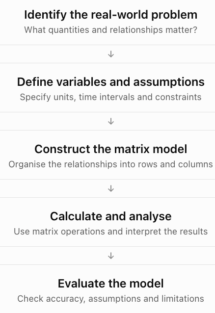
The calculations are only one part of the modelling process. A useful model must also make sense in the context of the original problem.
Transition Matrices
A transition matrix describes how a system changes from one state to another.
Transition matrices are particularly useful when individuals or quantities move between categories over time.
Examples include:
-
Customers switching between brands.
-
Students moving between courses.
-
Animals moving between habitats.
-
Workers changing employment categories.
-
Weather changing between sunny and rainy conditions.
-
Machines changing between operating states.
Understanding states
A state is a category or condition that a system can occupy.
For example, a simple weather model may have two states:
-
Sunny
-
Rainy
Suppose the probabilities of tomorrow's weather are:
|
Today's weather |
Sunny tomorrow |
Rainy tomorrow |
|---|---|---|
|
Sunny |
0.8 |
0.2 |
|
Rainy |
0.3 |
0.7 |
If today is sunny, there is an 80% probability that tomorrow will also be sunny.
If today is rainy, there is a 30% probability that tomorrow will be sunny.
Constructing a transition matrix
In this lesson, we use column state vectors and column-stochastic transition matrices.
This means:
-
Each column represents the current state.
-
Each row represents the next state.
-
Every column sums to 1.
The weather transition matrix is:
The first column represents transitions from sunny weather.
The second column represents transitions from rainy weather.
The columns sum to 1:
0.8 + 0.2 = 1
0.3 + 0.7 = 1
Some textbooks use row-stochastic matrices instead. Both conventions are valid, but the matrix and state-vector orientation must be consistent.
Transition Diagrams
A transition diagram shows states as circles and probabilities as arrows.
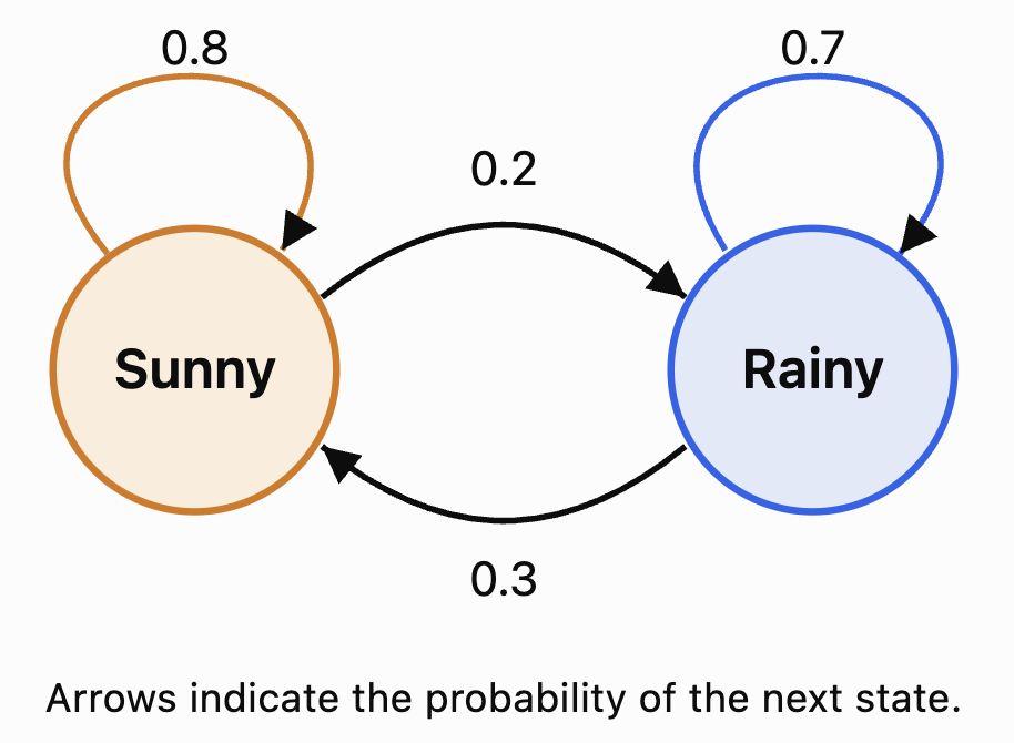
A transition diagram is useful because it provides a visual representation of the same information contained in the matrix.
State Vectors
A state vector describes the current distribution of a system across its states.
For example, suppose the probability of today's weather is:
70% sunny
30% rainy
The state vector is:
To calculate tomorrow's weather probabilities:
More generally:
where:
-
Sₙ is the state vector at time n.
-
T is the transition matrix.
-
Sₙ₊₁ is the state vector at the next time step.
Worked Example 1: Predicting Tomorrow's Weather
Given:
and:
Calculate:
Sunny:
0.8(0.7) + 0.3(0.3) = 0.65
Rainy:
0.2(0.7) + 0.7(0.3) = 0.35
Therefore:
Tomorrow's predicted probabilities are:
-
Sunny: 65%
-
Rainy: 35%
Check:
0.65 + 0.35 = 1
The probabilities are valid.
Repeated Transitions
To predict the state after two time periods:
Since S₁ = TS₀:
Therefore:
After n time periods:
This is one of the most important formulas in transition matrix modelling.
Worked Example 2: Weather After Two Days
Using the previous model:
Calculate:
Sunny:
0.8(0.65) + 0.3(0.35)
= 0.52 + 0.105
= 0.625
Rainy:
0.2(0.65) + 0.7(0.35)
= 0.13 + 0.245
= 0.375
Therefore:
After two days:
-
Sunny probability: 62.5%
-
Rainy probability: 37.5%
The model predicts a gradual movement towards a stable distribution.
Exploring a Transition Model
Use the interactive model below to change the transition probabilities and observe how the state distribution evolves.
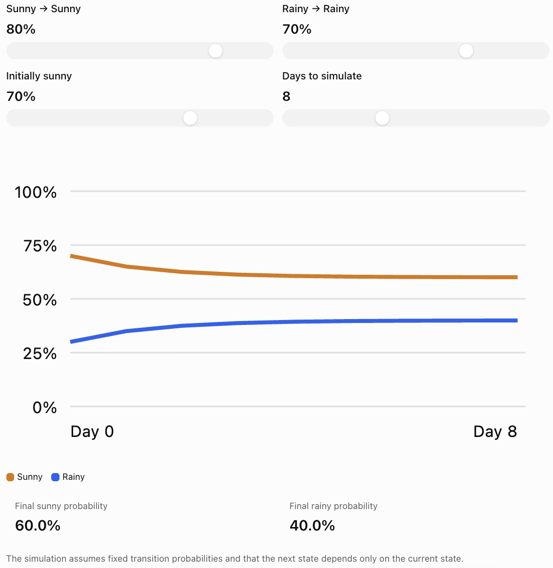
Notice that different starting distributions may approach the same long-term distribution, depending on the transition probabilities.
Steady-State Distributions
A steady-state distribution is a state vector that remains unchanged after applying the transition matrix.
If S is a steady-state vector:
This is also an eigenvector equation with eigenvalue 1.
For a probability transition matrix, the entries of S must be nonnegative and sum to 1.
Worked Example 3: Finding a Steady-State Distribution
Consider:
Let:
We require:
TS = S
Therefore:
0.8x + 0.3y = x
0.2x + 0.7y = y
Rearrange the first equation:
0.3y = 0.2x
Therefore:
3y = 2x
We also know:
x + y = 1
From 3y = 2x:
x = 1.5y
Substitute:
1.5y + y = 1
2.5y = 1
y = 0.4
Then:
x = 0.6
Therefore:
The steady-state distribution is:
-
Sunny: 60%
-
Rainy: 40%
Interpretation
Under this model, the long-term weather distribution approaches 60% sunny and 40% rainy, regardless of the initial probability distribution.
This convergence occurs because the transition matrix has suitable properties, including positive transition probabilities.
Not every transition matrix has a unique steady state or converges to one.
Markov Chains
A Markov chain is a mathematical model describing transitions between states in which the next state depends only on the current state.
This is called the Markov property.
For example, in a simplified weather model, tomorrow's weather depends on today's weather but not directly on the weather several days ago.
A Markov chain consists of:
-
A set of states.
-
Transition probabilities.
-
An initial state or probability distribution.
-
A rule for updating the distribution.
Transition matrices are a convenient way to represent finite Markov chains.
Limitations of Markov models
Real systems may depend on more information than the current state.
For example, weather also depends on:
-
Season
-
Temperature
-
Atmospheric pressure
-
Geographic location
-
Large-scale weather systems
A two-state model is therefore a simplified representation, not a complete weather forecasting system.
Real-World Application 1: Customer Brand Switching
Suppose a market contains two competing brands, A and B.
Each month:
-
85% of Brand A customers remain with A.
-
15% switch from A to B.
-
25% of Brand B customers switch to A.
-
75% remain with B.
The transition matrix is:
Suppose initially:
-
Brand A has 600 customers.
-
Brand B has 400 customers.
The initial state vector is:
Worked Example 4: Predicting Market Shares
Calculate:
Brand A:
0.85(600) + 0.25(400)
= 510 + 100
= 610
Brand B:
0.15(600) + 0.75(400)
= 90 + 300
= 390
Therefore:
After one month, the expected customer counts are:
-
Brand A: 610
-
Brand B: 390
The total remains 1,000.
Long-term interpretation
At steady state:
0.15x = 0.25y
Therefore:
3x = 5y
Since x + y = 1:
x = 0.625
y = 0.375
The long-term market shares are:
-
Brand A: 62.5%
-
Brand B: 37.5%
This assumes customers remain in the two-brand market and the transition probabilities remain constant.
Network Modelling
A network is a collection of objects connected by relationships.
Networks appear in many real-world situations:
-
Cities connected by roads.
-
Airports connected by flights.
-
People connected through social relationships.
-
Computers connected through communication links.
-
Power stations connected by transmission lines.
-
Webpages connected by hyperlinks.
In mathematics, networks are often represented using graphs.
A graph consists of:
-
Vertices (nodes): Objects in the network.
-
Edges: Connections between objects.
Matrices provide an efficient way to represent these connections.
Adjacency Matrices
An adjacency matrix records which vertices in a network are connected.
For a network with n vertices, its adjacency matrix is an n × n matrix.
For a simple undirected graph:
-
Entry 1 indicates a connection.
-
Entry 0 indicates no connection.
-
The matrix is symmetric.
-
Diagonal entries are zero when there are no self-loops.
Example Network
Suppose four locations are connected as follows:
-
A connects to B and C.
-
B connects to A, C, and D.
-
C connects to A and B.
-
D connects only to B.
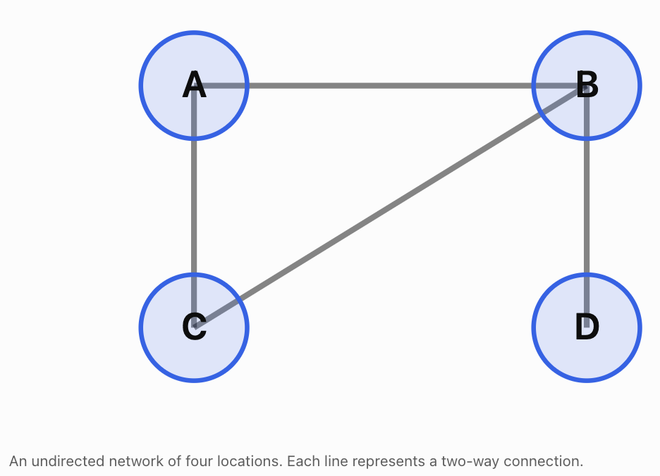
Using the order A, B, C, D, the adjacency matrix is:
\[ \boxed{ M=\begin{bmatrix} 0&1&1&0\\ 1&0&1&1\\ 1&1&0&0\\ 0&1&0&0 \end{bmatrix} } \]Interpreting the matrix
Row A:
0, 1, 1, 0
This means A connects to B and C.
Row B:
1, 0, 1, 1
This means B connects to A, C, and D.
Because the graph is undirected:
Mᵀ = M
The adjacency matrix is symmetric.
Degree of a Vertex
The degree of a vertex is the number of edges connected to it.
For a simple undirected graph, we can calculate the degree by adding the entries in its corresponding adjacency matrix row.
Using the previous network:
Degree of A = 2
Degree of B = 3
Degree of C = 2
Degree of D = 1
Vertex B has the greatest degree.
Therefore, B is the most directly connected vertex in this network.
This type of analysis is useful in transport planning, social networks, and communication systems.
Matrix Powers and Network Paths
An important property of adjacency matrices is that their powers contain information about walks through a network.
If M is the adjacency matrix of a graph, then:
The entry (i, j) of Mⁿ counts the number of walks of length n from vertex i to vertex j.
A walk may revisit vertices or edges, so it is not necessarily a simple path.
Worked Example 5: Counting Two-Step Walks
Consider a network with three vertices:
A — B — C
Its adjacency matrix is:
\[ M=\begin{bmatrix} 0&1&0\\ 1&0&1\\ 0&1&0 \end{bmatrix} \]Calculate M²:
\[ M^2= \begin{bmatrix} 0&1&0\\ 1&0&1\\ 0&1&0 \end{bmatrix} \begin{bmatrix} 0&1&0\\ 1&0&1\\ 0&1&0 \end{bmatrix} \]The result is:
\[ \boxed{ M^2=\begin{bmatrix} 1&0&1\\ 0&2&0\\ 1&0&1 \end{bmatrix} } \]Interpret the entry in row A, column C.
It equals 1.
Therefore, there is exactly one two-step walk from A to C:
A → B → C
The entry in row B, column B equals 2.
There are two two-step walks from B back to B:
B → A → B
B → C → B
This demonstrates how matrix multiplication can reveal indirect connections.
Directed Networks
Some networks contain connections that operate in only one direction.
Examples include:
-
One-way roads.
-
Flights operating in one direction.
-
Social media following relationships.
-
Webpage hyperlinks.
-
Supply chains.
These are called directed graphs.
For a directed graph, the adjacency matrix does not need to be symmetric.
Suppose:
A → B
B → C
C → A
The adjacency matrix is:
\[ M=\begin{bmatrix} 0&1&0\\ 0&0&1\\ 1&0&0 \end{bmatrix} \]Here, rows represent starting vertices and columns represent destination vertices.
For example:
M₁₂ = 1
means there is a directed edge from A to B.
But:
M₂₁ = 0
means there is no directed edge from B to A.
The direction of connections matters.
Weighted Networks
Not all connections are equally important.
Some networks assign numerical values to edges.
These values are called weights.
Weights may represent:
-
Distance
-
Travel time
-
Cost
-
Capacity
-
Strength of a relationship
-
Amount of information transferred
Example: Transport Network
Suppose three cities are connected by roads.
Route
Distance
A to B
40 km
A to C
70 km
B to C
30 km
A weighted adjacency matrix is:
\[ W=\begin{bmatrix} 0&40&70\\ 40&0&30\\ 70&30&0 \end{bmatrix} \]The entry in row A, column B is 40, indicating a distance of 40 km.
For this particular network, zero on the diagonal represents the distance from a city to itself.
When zero is also used to represent no connection, care is needed to distinguish missing routes from zero-weight routes.
Why weighted networks are useful
They allow us to investigate:
-
Shortest routes.
-
Lowest-cost connections.
-
Transport efficiency.
-
Communication capacity.
-
Resource distribution.
However, ordinary matrix multiplication does not directly calculate shortest routes. Shortest-path problems generally require specialised algorithms or alternative matrix operations.
Real-World Application 2: School Course Enrolment
A school offers three elective courses:
-
Art
-
Music
-
Technology
At the beginning of a semester, enrolment is:
Course
Students
Art
80
Music
60
Technology
100
The initial enrolment vector is:
\[ S_0=\begin{bmatrix}80\\60\\100\end{bmatrix} \]Suppose the school estimates the following transition percentages between semesters.
Current course
Next: Art
Next: Music
Next: Technology
Art
70%
20%
10%
Music
10%
80%
10%
Technology
20%
10%
70%
Using our column-vector convention, the transition matrix is:
\[ T=\begin{bmatrix} 0.7&0.1&0.2\\ 0.2&0.8&0.1\\ 0.1&0.1&0.7 \end{bmatrix} \]Worked Example 6: Predicting Enrolment
Calculate:
\[ S_1=TS_0 \]\[ S_1= \begin{bmatrix} 0.7&0.1&0.2\\ 0.2&0.8&0.1\\ 0.1&0.1&0.7 \end{bmatrix} \begin{bmatrix} 80\\60\\100 \end{bmatrix} \]Art:
0.7(80) + 0.1(60) + 0.2(100)
= 56 + 6 + 20
= 82
Music:
0.2(80) + 0.8(60) + 0.1(100)
= 16 + 48 + 10
= 74
Technology:
0.1(80) + 0.1(60) + 0.7(100)
= 8 + 6 + 70
= 84
Therefore:
\[ \boxed{S_1=\begin{bmatrix}82\\74\\84\end{bmatrix}} \]Interpretation
The model predicts:
-
Art: 82 students
-
Music: 74 students
-
Technology: 84 students
The total remains:
82 + 74 + 84 = 240
This agrees with the original total of 240 students.
Evaluating the model
The model assumes:
-
Students select exactly one of these electives.
-
No students enter or leave the group.
-
The transition probabilities remain constant.
-
Student decisions can be represented using the estimated percentages.
In reality, course popularity, teacher availability, timetabling, and student preferences may change.
Therefore, the predictions should be treated as estimates.
Real-World Application 3: Input–Output Economic Models
Matrices can describe how different industries depend on one another.
For example, agriculture may require manufacturing products, while manufacturing may require agricultural resources.
These relationships can be represented using an input–output model.
Suppose an economy has two industries:
-
Agriculture
-
Manufacturing
For each unit of agricultural output, production requires:
-
0.2 units of agricultural output.
-
0.1 units of manufacturing output.
For each unit of manufacturing output, production requires:
-
0.3 units of agricultural output.
-
0.2 units of manufacturing output.
The input coefficient matrix is:
\[ A=\begin{bmatrix} 0.2&0.3\\ 0.1&0.2 \end{bmatrix} \]The columns represent the industries producing output, while the rows represent the inputs required.
Suppose final consumer demand is:
\[ D=\begin{bmatrix}100\\80\end{bmatrix} \]Let X represent the total production required.
The model is:
\[ X=AX+D \]Rearrange:
\[ X-AX=D \]\[ (I-A)X=D \]Therefore:
\[ \boxed{X=(I-A)^{-1}D} \]provided I − A is invertible.
Worked Example 7: Calculating Required Production
First:
\[ I-A= \begin{bmatrix} 0.8&-0.3\\ -0.1&0.8 \end{bmatrix} \]Calculate the determinant:
det(I − A) = 0.8(0.8) − (−0.3)(−0.1)
= 0.64 − 0.03
= 0.61
Therefore:
\[ (I-A)^{-1}= \frac1{0.61} \begin{bmatrix} 0.8&0.3\\ 0.1&0.8 \end{bmatrix} \]Multiply:
\[ X=\frac1{0.61} \begin{bmatrix} 0.8&0.3\\ 0.1&0.8 \end{bmatrix} \begin{bmatrix}100\\80\end{bmatrix} \]\[ X=\frac1{0.61} \begin{bmatrix} 104\\74 \end{bmatrix} \]Therefore:
\[ \boxed{ X\approx\begin{bmatrix} 170.49\\ 121.31 \end{bmatrix} } \]The economy must produce approximately:
-
170.49 units of agricultural output.
-
121.31 units of manufacturing output.
These totals exceed final consumer demand because each industry also supplies inputs needed for production.
This simplified model assumes fixed input requirements and sufficient production capacity.
Analysing Matrix-Based Systems
Once a matrix model has been constructed, we can investigate more than its immediate numerical results.
We can examine its stability, sensitivity, connectivity, and long-term behaviour.
Stability
A system is stable when its behaviour remains controlled or approaches a predictable state.
For a repeated linear system:
\[ X_{n+1}=AX_n \]the magnitudes of eigenvalues help determine long-term behaviour.
-
Eigenvalues with absolute value less than 1 correspond to directions that decay.
-
Eigenvalues with absolute value greater than 1 correspond to directions that grow.
-
Eigenvalues with absolute value equal to 1 require closer analysis.
If all eigenvalues have absolute value less than 1, then repeated application of A drives every state vector towards zero.
Transition matrices behave differently because they have an eigenvalue of 1, and may approach a nonzero steady-state distribution.
Sensitivity
A model is sensitive when small changes in inputs or assumptions produce large changes in its predictions.
For example, changing a customer retention rate from 85% to 80% may affect long-term market shares substantially.
Sensitivity analysis helps answer questions such as:
-
What happens if costs increase?
-
What happens if transition probabilities change?
-
What happens if demand rises?
-
Which assumptions have the greatest influence?
Connectivity
In network models, we can investigate how well the system is connected.
Useful measurements include:
-
Degree of a vertex.
-
Number of walks between vertices.
-
Whether one vertex can be reached from another.
-
Importance of particular connections.
-
Whether removing an edge disconnects part of the network.
Model validity
A matrix calculation may be mathematically correct but still produce a poor real-world prediction.
A model should be evaluated by asking:
-
Are the assumptions realistic?
-
Are the input values reliable?
-
Are the units consistent?
-
Are important factors missing?
-
Does the model agree with observed data?
-
How far into the future can the predictions reasonably be trusted?
Worked Example 8: Evaluating a Population Model
A population contains two groups of animals.
The population changes according to:
\[ X_{n+1}= \begin{bmatrix} 0.8&0\\ 0&1.2 \end{bmatrix}X_n \]Initially:
\[ X_0=\begin{bmatrix}100\\50\end{bmatrix} \]Calculate the population after two periods.
Step 1: Calculate the first period.
\[ X_1= \begin{bmatrix} 0.8&0\\ 0&1.2 \end{bmatrix} \begin{bmatrix}100\\50\end{bmatrix} \]\[ X_1=\begin{bmatrix}80\\60\end{bmatrix} \]Step 2: Calculate the second period.
\[ X_2= \begin{bmatrix} 0.8&0\\ 0&1.2 \end{bmatrix} \begin{bmatrix}80\\60\end{bmatrix} \]\[ \boxed{X_2=\begin{bmatrix}64\\72\end{bmatrix}} \]Interpretation
The first group decreases by 20% each period.
The second group increases by 20% each period.
The eigenvalues are:
λ₁ = 0.8
λ₂ = 1.2
These values explain the different long-term behaviours.
Limitations
The model assumes fixed growth rates and no interaction between the groups.
Real populations may be affected by food availability, disease, migration, competition, and environmental changes.
Choosing an Appropriate Matrix Model
Different problems require different types of matrices.
Situation
Suitable model
Calculating resources for production
Resource coefficient matrix
Predicting movement between categories
Transition matrix
Representing connections between locations
Adjacency matrix
Representing distances or costs
Weighted network matrix
Analysing relationships between industries
Input–output matrix
Predicting repeated growth or decay
Repeated matrix transformation
Finding long-term probability distributions
Steady-state transition model
The most important modelling decision is identifying what the rows, columns, and matrix entries represent.
A well-constructed matrix model should have a clear interpretation for every entry.
Common Mistakes
Mistake 1: Reversing rows and columns in a transition matrix
Always establish whether rows or columns represent the current state.
Mistake 2: Forgetting that transition probabilities must sum to 1
Under the column-stochastic convention, each column must sum to 1.
Mistake 3: Multiplying matrices in the wrong order
For column state vectors, use Sₙ₊₁ = TSₙ.
Mistake 4: Confusing a state vector with a transition matrix
The state vector describes the current distribution. The transition matrix describes how that distribution changes.
Mistake 5: Assuming all transition matrices converge to one steady state
Some systems cycle or have multiple steady states.
Mistake 6: Confusing paths and walks
Matrix powers count walks, which may revisit vertices or edges.
Mistake 7: Assuming adjacency matrices must be symmetric
Only undirected networks have symmetric adjacency matrices under the standard convention.
Mistake 8: Confusing weighted networks with ordinary adjacency matrices
Weighted matrices contain values such as distances or costs, not simply zeros and ones.
Mistake 9: Ignoring units
A resource matrix may contain hours, kilograms, or monetary amounts. These must be interpreted consistently.
Mistake 10: Assuming model predictions are guaranteed outcomes
Models describe expected or estimated behaviour based on assumptions.
Mistake 11: Applying matrix operations without checking dimensions
Matrix multiplication requires compatible dimensions.
Mistake 12: Ignoring model limitations
Real systems may contain factors not represented by the matrix.
Key Terms
-
Matrix Model: Mathematical representation of a system using matrices.
-
State: Category or condition occupied by a system.
-
State Vector: Vector describing the current distribution across states.
-
Transition Matrix: Matrix describing movement between states.
-
Transition Probability: Probability of moving from one state to another.
-
Column-Stochastic Matrix: Nonnegative matrix whose columns each sum to 1.
-
Row-Stochastic Matrix: Nonnegative matrix whose rows each sum to 1.
-
Markov Chain: Model in which the next state depends only on the current state.
-
Markov Property: Assumption that future transitions depend only on the present state.
-
Steady-State Distribution: Probability distribution unchanged by the transition matrix.
-
Matrix Power: Repeated multiplication of a matrix by itself.
-
Network: Collection of objects connected by relationships.
-
Graph: Mathematical structure consisting of vertices and edges.
-
Vertex: Node representing an object in a network.
-
Edge: Connection between two vertices.
-
Adjacency Matrix: Matrix recording connections between vertices.
-
Directed Graph: Graph whose edges have directions.
-
Undirected Graph: Graph whose edges do not have directions.
-
Weighted Graph: Graph whose edges have numerical values.
-
Degree: Number of edges incident to a vertex in an undirected graph.
-
Walk: Sequence of connected vertices that may repeat vertices or edges.
-
Path: Walk with no repeated vertices, under the standard simple-path definition.
-
Connectivity: Description of how vertices are linked.
-
Input–Output Model: Economic model describing relationships between industries.
-
Eigenvalue: Scalar describing how an eigenvector is scaled.
-
Stability: Behaviour of a system over time.
-
Sensitivity Analysis: Investigation of how changes in inputs affect outputs.
-
Model Assumption: Simplification or condition used to construct a model.
-
Model Validation: Process of comparing a model with real-world observations.
Key Takeaways
-
Matrices can represent practical systems involving several related quantities.
-
Matrix multiplication can calculate resource requirements and other outputs.
-
Transition matrices describe movement between states.
-
State vectors represent the current distribution of a system.
-
Repeated transitions are calculated using Sₙ = TⁿS₀.
-
A steady-state distribution satisfies TS = S.
-
Markov chains describe transitions that depend only on the current state.
-
Networks can be represented using adjacency matrices.
-
Matrix powers can count walks of specified lengths in a network.
-
Directed networks may have non-symmetric adjacency matrices.
-
Weighted networks represent quantities such as distance, cost, or capacity.
-
Matrix models can describe population changes, market shares, and economic relationships.
-
Eigenvalues help explain growth, decay, and stability.
-
Mathematical models depend on assumptions and may not perfectly represent reality.
-
Results must always be interpreted in the context of the original problem.
Check Your Understanding
Questions
Question 1: Resource Modelling
A factory produces two products.
Product A requires 3 labour hours and 4 material units.
Product B requires 5 labour hours and 2 material units.
Write the resource matrix.
Question 2: Matrix Multiplication
Using Question 1, calculate the resources required to produce 10 units of A and 20 units of B.
Question 3: Transition Matrix
A system has two states, A and B.
-
80% of A remains in A.
-
20% of A moves to B.
-
30% of B moves to A.
-
70% of B remains in B.
Write the column-stochastic transition matrix.
Question 4: One-Step Transition
Using Question 3, calculate the next state if:
\[ S_0=\begin{bmatrix}100\\200\end{bmatrix} \]Question 5: Two-Step Transition
Using the same transition matrix and initial state, calculate S₂.
Question 6: Steady State
Find the steady-state probability distribution for:
\[ T=\begin{bmatrix} 0.7&0.2\\ 0.3&0.8 \end{bmatrix} \]Question 7: Adjacency Matrix
A network contains three vertices:
A connects to B.
B connects to A and C.
C connects to B.
Write its adjacency matrix.
Question 8: Vertex Degree
Using Question 7, determine the degree of each vertex.
Question 9: Matrix Powers
Calculate M² for the adjacency matrix in Question 7.
Interpret the entry in row A, column C.
Question 10: Directed Network
A directed network has connections:
A → B
B → C
C → A
Write its adjacency matrix.
Question 11: Weighted Network
Three cities have the following direct road distances:
A–B: 50 km
A–C: 80 km
B–C: 40 km
Write a symmetric weighted adjacency matrix.
Question 12: Population Model
A population is modelled by:
\[ X_{n+1}= \begin{bmatrix} 0.9&0\\ 0&1.1 \end{bmatrix}X_n \]If:
\[ X_0=\begin{bmatrix}200\\100\end{bmatrix} \]calculate X₂.
Question 13: Economic Modelling
An economy has:
\[ A=\begin{bmatrix} 0.2&0\\ 0&0.25 \end{bmatrix} \]and final demand:
\[ D=\begin{bmatrix}80\\60\end{bmatrix} \]Solve X = AX + D.
Question 14: Evaluating Models
Explain three limitations of using a fixed transition matrix to predict customer behaviour over several years.
Question 15: Integrated Challenge
A school has 500 students choosing between two clubs, Science and Mathematics.
Initially:
-
300 students choose Science.
-
200 students choose Mathematics.
Each semester:
-
80% of Science students remain in Science.
-
20% move to Mathematics.
-
30% of Mathematics students move to Science.
-
70% remain in Mathematics.
a) Construct the transition matrix.
b) Write the initial state vector.
c) Calculate the expected club membership after one semester.
d) Calculate the expected membership after two semesters.
e) Find the steady-state distribution.
f) Explain two assumptions of the model.
Fully Worked Answers
Answer 1: Resource Modelling
Rows represent labour and materials.
Columns represent Products A and B.
\[ \boxed{ R=\begin{bmatrix} 3&5\\ 4&2 \end{bmatrix} } \]Answer 2: Matrix Multiplication
Production vector:
\[ P=\begin{bmatrix}10\\20\end{bmatrix} \]Calculate:
\[ RP= \begin{bmatrix} 3&5\\ 4&2 \end{bmatrix} \begin{bmatrix}10\\20\end{bmatrix} \]Labour:
3(10) + 5(20) = 130
Materials:
4(10) + 2(20) = 80
\[ \boxed{RP=\begin{bmatrix}130\\80\end{bmatrix}} \]Answer: 130 labour hours and 80 material units.
Answer 3: Transition Matrix
Using columns for current states:
\[ \boxed{ T=\begin{bmatrix} 0.8&0.3\\ 0.2&0.7 \end{bmatrix} } \]Each column sums to 1.
Answer 4: One-Step Transition
\[ S_1=TS_0 \]\[ S_1= \begin{bmatrix} 0.8&0.3\\ 0.2&0.7 \end{bmatrix} \begin{bmatrix}100\\200\end{bmatrix} \]First component:
0.8(100) + 0.3(200) = 140
Second component:
0.2(100) + 0.7(200) = 160
\[ \boxed{S_1=\begin{bmatrix}140\\160\end{bmatrix}} \]Answer 5: Two-Step Transition
Use the result from Question 4:
\[ S_1=\begin{bmatrix}140\\160\end{bmatrix} \]Then:
\[ S_2=TS_1 \]First component:
0.8(140) + 0.3(160) = 160
Second component:
0.2(140) + 0.7(160) = 140
\[ \boxed{S_2=\begin{bmatrix}160\\140\end{bmatrix}} \]Answer 6: Steady State
Given:
\[ T=\begin{bmatrix}0.7&0.2\\0.3&0.8\end{bmatrix} \]Let:
\[ S=\begin{bmatrix}x\\y\end{bmatrix} \]Solve:
TS = S
From the first row:
0.7x + 0.2y = x
Therefore:
0.2y = 0.3x
2y = 3x
y = 1.5x
Also:
x + y = 1
Therefore:
x + 1.5x = 1
2.5x = 1
x = 0.4
y = 0.6
\[ \boxed{S=\begin{bmatrix}0.4\\0.6\end{bmatrix}} \]Answer: 40% in A and 60% in B.
Answer 7: Adjacency Matrix
Connections:
A–B
B–C
The adjacency matrix is:
\[ \boxed{ M=\begin{bmatrix} 0&1&0\\ 1&0&1\\ 0&1&0 \end{bmatrix} } \]Answer 8: Vertex Degree
Add the entries in each row.
A: 0 + 1 + 0 = 1
B: 1 + 0 + 1 = 2
C: 0 + 1 + 0 = 1
Answer: Degree(A) = 1, Degree(B) = 2, Degree(C) = 1.
Answer 9: Matrix Powers
\[ M=\begin{bmatrix} 0&1&0\\ 1&0&1\\ 0&1&0 \end{bmatrix} \]Multiplying M by itself gives:
\[ \boxed{ M^2=\begin{bmatrix} 1&0&1\\ 0&2&0\\ 1&0&1 \end{bmatrix} } \]The entry in row A, column C equals 1.
Therefore, there is one two-step walk from A to C:
A → B → C
Answer 10: Directed Network
Using rows as starting vertices and columns as destinations:
\[ \boxed{ M=\begin{bmatrix} 0&1&0\\ 0&0&1\\ 1&0&0 \end{bmatrix} } \]This matrix is not symmetric because the connections are directed.
Answer 11: Weighted Network
Using the order A, B, C:
\[ \boxed{ W=\begin{bmatrix} 0&50&80\\ 50&0&40\\ 80&40&0 \end{bmatrix} } \]The matrix is symmetric because the distances are the same in both directions.
Answer 12: Population Model
Given:
\[ A=\begin{bmatrix}0.9&0\\0&1.1\end{bmatrix} \]and:
\[ X_0=\begin{bmatrix}200\\100\end{bmatrix} \]After one period:
\[ X_1=\begin{bmatrix}180\\110\end{bmatrix} \]After two periods:
\[ X_2=AX_1 \]\[ X_2= \begin{bmatrix} 0.9(180)\\ 1.1(110) \end{bmatrix} \]\[ \boxed{X_2=\begin{bmatrix}162\\121\end{bmatrix}} \]The first group decreases while the second increases.
Answer 13: Economic Modelling
Given:
\[ A=\begin{bmatrix}0.2&0\\0&0.25\end{bmatrix} \]and:
\[ D=\begin{bmatrix}80\\60\end{bmatrix} \]The model is:
X = AX + D
Therefore:
(I − A)X = D
\[ I-A=\begin{bmatrix}0.8&0\\0&0.75\end{bmatrix} \]This gives:
0.8x = 80
0.75y = 60
Therefore:
x = 100
y = 80
\[ \boxed{X=\begin{bmatrix}100\\80\end{bmatrix}} \]Answer 14: Evaluating Models
Three limitations include:
-
Changing preferences: Customer choices may change because of advertising, prices, or new products.
-
Fixed probabilities: The model assumes transition probabilities remain constant, which may be unrealistic over several years.
-
Missing factors: Economic conditions, competitors, and population changes may affect customer behaviour.
Therefore, predictions become less reliable if the model assumptions no longer reflect reality.
Answer 15: Integrated Challenge
Part a: Transition matrix
Using Science first and Mathematics second:
\[ \boxed{ T=\begin{bmatrix} 0.8&0.3\\ 0.2&0.7 \end{bmatrix} } \]Part b: Initial state vector
\[ \boxed{ S_0=\begin{bmatrix}300\\200\end{bmatrix} } \]Part c: After one semester
\[ S_1=TS_0 \]Science:
0.8(300) + 0.3(200)
= 240 + 60
= 300
Mathematics:
0.2(300) + 0.7(200)
= 60 + 140
= 200
Therefore:
\[ \boxed{S_1=\begin{bmatrix}300\\200\end{bmatrix}} \]The membership distribution remains unchanged.
Part d: After two semesters
Since S₁ = S₀:
\[ S_2=TS_1 \]\[ \boxed{S_2=\begin{bmatrix}300\\200\end{bmatrix}} \]The distribution remains unchanged again.
Part e: Steady-state distribution
Let:
\[ S=\begin{bmatrix}x\\y\end{bmatrix} \]Solve:
TS = S
From the first row:
0.8x + 0.3y = x
Therefore:
0.3y = 0.2x
3y = 2x
x = 1.5y
Since:
x + y = 1
1.5y + y = 1
2.5y = 1
y = 0.4
x = 0.6
Therefore:
\[ \boxed{S=\begin{bmatrix}0.6\\0.4\end{bmatrix}} \]The steady-state distribution is:
-
Science: 60%
-
Mathematics: 40%
For 500 students:
Science = 0.6(500) = 300
Mathematics = 0.4(500) = 200
The initial distribution was already at steady state.
Part f: Assumptions
Two assumptions are:
-
The total number of students remains constant at 500.
-
The transition percentages remain unchanged each semester.
Other assumptions include that students belong to exactly one of the two clubs and that movement depends only on their current club.
Final Reflection
Matrix modelling allows complex real-world systems to be represented using organised mathematical structures.
Transition matrices describe movement between categories, while adjacency matrices represent connections within networks. Weighted matrices extend these ideas by including distances, costs, capacities, and other numerical relationships.
Matrix multiplication allows us to predict future states, calculate resource requirements, and analyse indirect network connections.
Repeated matrix operations reveal how systems change over time, while steady-state analysis and eigenvalues help explain long-term behaviour.
However, mathematical modelling requires more than correct calculations. A useful model must be based on reasonable assumptions, interpreted carefully, and evaluated against real-world evidence.
The central idea is that matrices transform complicated relationships into mathematical models that can be used to describe systems, analyse their behaviour, make predictions, and support practical decisions.
-