Matrix Transformations and Applications

Introduction

When a matrix transforms a vector, it usually changes both the vector's length and its direction. However, some vectors behave differently: after the transformation, they remain on the same line through the origin.

These special vectors are called eigenvectors, and the numbers describing how they are scaled are called eigenvalues.

Eigenvalues and eigenvectors are important because they reveal the underlying behaviour of matrix transformations. They help mathematicians and scientists understand how systems change, which directions remain unchanged, and whether processes grow, shrink, or remain stable.

They are used in many areas, including:

• Physics: vibrations, forces, and quantum mechanics.

• Engineering: structural stability and mechanical systems.

• Computer science: image processing and machine learning.

• Biology: population growth and ecological models.

• Economics: long-term behaviour of economic systems.

• Data science: principal component analysis and dimensionality reduction.

In this lesson, we will investigate how to identify, calculate, and interpret eigenvalues and eigenvectors, beginning with simple 2 × 2 matrices and progressing to practical applications.

What Are Eigenvalues and Eigenvectors?

Consider a square matrix A acting on a nonzero vector v.

Normally, multiplying A by v changes the direction and magnitude of v.

However, for certain vectors, the result is simply a scalar multiple of the original vector.

This relationship is written as:

where:

• A is a square matrix representing a linear transformation.

• v is a nonzero eigenvector.

• λ (lambda) is the corresponding eigenvalue.

• Av is the transformed vector.

An eigenvector is a nonzero vector whose direction stays on the same line after the transformation.

An eigenvalue is the scalar by which that eigenvector is multiplied.

Interpreting the eigenvalue

The eigenvector must be nonzero. Otherwise, every matrix would trivially satisfy A0 = λ0 for any λ.

A Geometric Illustration

Consider the transformation:

This stretches the x-direction by a factor of 2 and compresses the y-direction by a factor of 1/2.

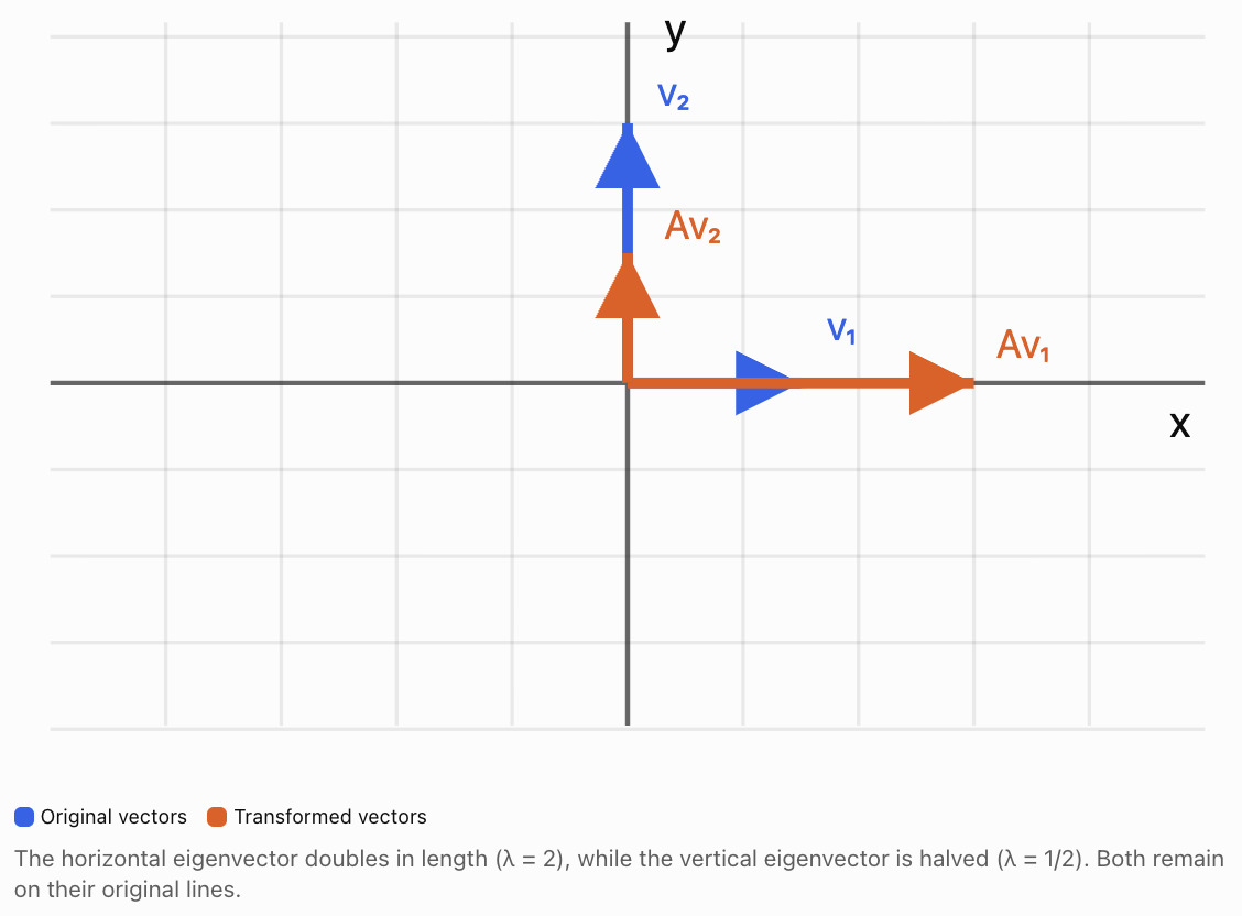
The x-axis and y-axis are special directions for this transformation.

Any nonzero vector along the x-axis is an eigenvector with eigenvalue 2.

Any nonzero vector along the y-axis is an eigenvector with eigenvalue 1/2.

Vectors that do not lie along these axes generally change direction.

Identifying Eigenvalues from Simple Matrices

Some matrices have eigenvalues that can be recognised immediately.

Diagonal matrices

Consider:

The matrix multiplies horizontal components by 4 and vertical components by 3.

Therefore:

• λ₁ = 4, corresponding to horizontal eigenvectors.

• λ₂ = 3, corresponding to vertical eigenvectors.

For a diagonal matrix, the diagonal entries are its eigenvalues.

Identity matrix

For every vector v:

Iv = v

Therefore, every nonzero vector is an eigenvector with eigenvalue 1.

Zero matrix

For every vector v:

Ov = 0v

Therefore, every nonzero vector is an eigenvector with eigenvalue 0.

Calculating Eigenvalues

For a general matrix, eigenvalues can be found using the characteristic equation.

Start with:

Since I is the identity matrix:

Rearrange:

For a nonzero solution v to exist, the matrix A − λI must be singular.

Therefore:

This is called the characteristic equation.

The expression det(A − λI) is the characteristic polynomial.

Its roots are the eigenvalues.

General formula for a 2 × 2 matrix

Let:

Then:

Calculate the determinant:

Expand:

ad − aλ − dλ + λ² − bc = 0

Rearrange:

Since a + d is the trace of A and ad − bc is its determinant:

This provides a useful connection between eigenvalues, trace, and determinant.

Worked Example 1: Calculating Eigenvalues

Find the eigenvalues of:

Step 1: Construct A − λI.

Step 2: Calculate the determinant.

Expand:

9 − 6λ + λ² − 1 = 0

Therefore:

λ² − 6λ + 8 = 0

Step 3: Factorise.

(λ − 2)(λ − 4) = 0

Therefore:

These are the eigenvalues of A.

Verification using trace and determinant

Trace:

tr(A) = 3 + 3 = 6

Sum of eigenvalues:

2 + 4 = 6

Determinant:

det(A) = 3(3) − 1(1) = 8

Product of eigenvalues:

2 × 4 = 8

Both relationships are satisfied.

Calculating Eigenvectors

After finding an eigenvalue, we determine its corresponding eigenvectors.

We use:

For a 2 × 2 matrix, write:

Substitute the eigenvalue and solve the resulting homogeneous system.

Eigenvectors are not unique.

If v is an eigenvector, then any nonzero scalar multiple kv is also an eigenvector corresponding to the same eigenvalue.

The set of all eigenvectors associated with an eigenvalue, together with the zero vector, forms an eigenspace.

Worked Example 2: Finding Corresponding Eigenvectors

Continue with:

We found:

λ₁ = 2

λ₂ = 4

Eigenvector for λ = 2

Substitute into:

(A − 2I)v = 0

This gives:

x + y = 0

Therefore:

y = −x

Choose x = 1.

Then y = −1.

An eigenvector is:

Any nonzero multiple of this vector is also valid.

Eigenvector for λ = 4

Substitute into:

(A − 4I)v = 0

This gives:

−x + y = 0

Therefore:

y = x

Choose x = 1.

Then y = 1.

An eigenvector is:

Verification

For v₁:

For v₂:

Both eigenvectors are correct.

Geometric Meaning of Eigenvectors

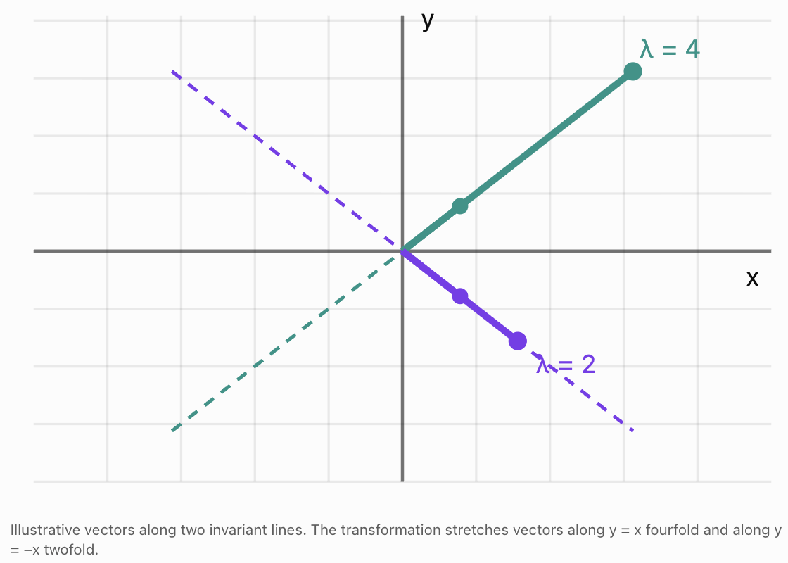
Eigenvectors identify directions that are preserved by a linear transformation, although the vector may reverse direction or become zero.

Consider again:

Its eigenvectors lie along:

y = x

and:

y = −x

Along y = x, the matrix stretches vectors by factor 4.

Along y = −x, it stretches vectors by factor 2.

Why this is important

A complicated transformation may behave simply along its eigenvector directions.

If we can identify those directions, we can understand the transformation more easily.

This becomes especially useful when the same matrix is applied repeatedly.

Worked Example 3: A Matrix with a Negative Eigenvalue

Consider:

The eigenvalues are:

λ₁ = −2

λ₂ = 3

For λ₁ = −2, an eigenvector is:

Apply the matrix:

The vector doubles in length and reverses direction.

For λ₂ = 3:

Apply the matrix:

The vector triples in length without reversing direction.

A negative eigenvalue therefore indicates reversal along the corresponding eigenvector line.

Repeated Matrix Transformations

Eigenvalues are particularly useful when the same transformation is applied repeatedly.

Suppose:

Apply A again:

Since λ is a scalar:

Therefore:

Repeating this process gives:

This means we can predict the effect of repeated transformations on eigenvectors without calculating large matrix powers.

Worked Example 4: Repeated Transformations

Suppose:

Find A⁴v.

Using the eigenvalue relationship:

A⁴v = 3⁴v

Therefore:

After four applications, the vector is 81 times its original length, with the same direction.

Growth and decay

If |λ| > 1, repeated transformations increase the vector's magnitude.

If 0 < |λ| < 1, repeated transformations decrease its magnitude.

If |λ| = 1, the magnitude remains unchanged.

If λ = 0, the vector becomes zero after one transformation.

Negative eigenvalues cause the direction to alternate with successive transformations.

Eigenvalues and Matrix Properties

Eigenvalues are connected to several important properties of matrices.

Trace and eigenvalues

For a 2 × 2 matrix:

the trace is:

tr(A) = a + d

The sum of the eigenvalues, counting multiplicity, is:

Determinant and eigenvalues

The product of the eigenvalues is:

Worked Example 5: Using Trace and Determinant

A 2 × 2 matrix has:

tr(A) = 9

det(A) = 20

Find its eigenvalues.

We know:

λ₁ + λ₂ = 9

λ₁λ₂ = 20

The characteristic equation is:

λ² − 9λ + 20 = 0

Factorise:

(λ − 4)(λ − 5) = 0

Therefore:

This method avoids calculating the characteristic determinant from scratch.

Eigenvalues and Singular Matrices

A square matrix is singular if its determinant is zero.

Since the determinant equals the product of the eigenvalues:

for a 2 × 2 matrix, if either eigenvalue is zero:

det(A) = 0

Therefore, the matrix is singular.

Worked Example 6: A Zero Eigenvalue

Consider:

Calculate the determinant:

det(A) = 2(2) − 4(1)

= 0

The matrix is singular.

Its characteristic equation is:

λ² − 4λ = 0

Factorise:

λ(λ − 4) = 0

Therefore:

The zero eigenvalue indicates that some nonzero vectors are transformed into the zero vector.

For example:

Then:

This confirms that v is an eigenvector with eigenvalue zero.

Matrices with Repeated Eigenvalues

A matrix may have the same eigenvalue more than once.

Consider:

Its characteristic equation is:

(3 − λ)² = 0

Therefore:

λ = 3 is a repeated eigenvalue.

Every nonzero vector is an eigenvector because:

Av = 3v

However, repeated eigenvalues do not always mean every vector is an eigenvector.

For example:

also has eigenvalue 3 repeated twice.

But:

The eigenvector equation gives:

y = 0

Therefore, its eigenvectors are only the nonzero vectors along the x-axis.

This distinction becomes important when studying diagonalisation.

Eigenvalues and Diagonalisation

Some matrices can be rewritten in a simpler form using their eigenvectors.

If a 2 × 2 matrix has two linearly independent eigenvectors, we can form a matrix P using those eigenvectors as columns.

The matrix can then be expressed as:

where D is a diagonal matrix containing the corresponding eigenvalues.

For example, if:

λ₁ = 2

λ₂ = 5

then:

Diagonalisation is useful because powers of diagonal matrices are easy to calculate:

Therefore:

This provides an efficient method for studying repeated transformations and long-term behaviour.

Not every matrix is diagonalizable, but many important matrices are.

Complex Eigenvalues

Not every real matrix has real eigenvalues.

Consider a rotation through 90° counterclockwise:

Its characteristic equation is:

λ² + 1 = 0

Therefore:

λ² = −1

The eigenvalues are:

where i² = −1.

This explains why a 90° rotation has no nonzero real eigenvectors: every nonzero real vector changes direction.

Complex eigenvalues are important in advanced mathematics, oscillations, electrical engineering, and dynamical systems.

Real-World Application 1: Population Growth

Eigenvalues can be used to predict how populations change over time.

Consider a simplified population divided into two age groups:

• Juveniles

• Adults

Suppose the population changes each year according to:

The matrix describes reproduction and survival.

Its characteristic equation is:

Therefore:

−λ(0.5 − λ) − 1 = 0

λ² − 0.5λ − 1 = 0

Using the quadratic formula:

Approximately:

λ₁ ≈ 1.281

λ₂ ≈ −0.781

The dominant eigenvalue is approximately 1.281.

In this simplified model, the long-term population grows by approximately 28.1% per year, provided the model remains valid and the initial population has a positive contribution along the dominant eigenvector.

The corresponding eigenvector describes the stable proportion of juveniles and adults approached over time.

Why this matters

Population models can help scientists investigate:

• Species conservation

• Wildlife management

• Fisheries

• Age distributions

• Long-term population trends

The results depend on the assumptions and accuracy of the model.

Real-World Application 2: Mechanical Vibrations

Engineers study how buildings, bridges, vehicles, and machines vibrate.

A mechanical system may have several possible vibration patterns.

Each natural vibration pattern is called a mode shape.

Eigenvectors describe these mode shapes, while eigenvalues are related to the corresponding natural frequencies.

For a simple undamped system:

where:

• K is the stiffness matrix.

• M is the mass matrix.

• v is a mode shape.

• ω is the angular frequency.

This is a generalised eigenvalue problem.

Engineers use these calculations to help prevent dangerous resonance and improve structural designs.

Real-World Application 3: Data Science and Principal Component Analysis

Principal component analysis (PCA) is a technique used to identify important patterns in data.

Suppose a dataset contains two related variables, such as height and arm span.

The data points may form an elongated cloud.

A covariance matrix describes how the variables vary together.

The eigenvectors of this matrix identify the principal directions of variation.

The corresponding eigenvalues describe how much variance lies along those directions.

The eigenvector with the largest eigenvalue identifies the direction of greatest variation.

This is useful for:

• Reducing the number of variables in datasets.

• Visualising high-dimensional data.

• Identifying patterns.

• Compressing information.

• Preparing data for machine learning.

Real-World Application 4: Search Engines and Networks

Large networks can be represented using matrices.

For example, a network may represent:

• Webpages and hyperlinks.

• People and social connections.

• Transport routes.

• Communication systems.

Eigenvectors can help identify important or influential nodes in a network.

In eigenvector centrality, a node is considered important when it is connected to other important nodes.

Related ideas are used in ranking algorithms and network analysis.

Common Mistakes

Mistake 1: Confusing eigenvalues with eigenvectors

An eigenvalue is a scalar. An eigenvector is a nonzero vector.

Mistake 2: Forgetting that eigenvectors must be nonzero

The zero vector is not an eigenvector.

Mistake 3: Calculating det(A) instead of det(A − λI)

The characteristic equation requires subtracting λ from the diagonal entries.

Mistake 4: Making sign errors in determinants

For a 2 × 2 matrix, the determinant is ad − bc.

Mistake 5: Finding eigenvalues but not eigenvectors

Each eigenvalue must be substituted into (A − λI)v = 0 to find corresponding eigenvectors.

Mistake 6: Assuming eigenvectors are unique

Any nonzero scalar multiple of an eigenvector is also an eigenvector.

Mistake 7: Assuming all matrices have real eigenvalues

Some real matrices have complex eigenvalues.

Mistake 8: Assuming every vector is an eigenvector

Only vectors satisfying Av = λv for some scalar λ are eigenvectors.

Mistake 9: Misinterpreting negative eigenvalues

A negative eigenvalue reverses direction along the eigenvector line.

Mistake 10: Assuming repeated eigenvalues always provide multiple independent eigenvectors

Some matrices have repeated eigenvalues but only one independent eigenvector.

Mistake 11: Forgetting to verify eigenvectors

Always check Av = λv.

Mistake 12: Confusing eigenvalue magnitude with vector length

The eigenvalue is a scaling factor, not necessarily the length of the eigenvector.

Key Terms

• Eigenvalue: Scalar describing how an eigenvector is scaled by a matrix.

• Eigenvector: Nonzero vector transformed into a scalar multiple of itself.

• Linear Transformation: Transformation preserving vector addition and scalar multiplication.

• Characteristic Equation: Equation det(A − λI) = 0 used to find eigenvalues.

• Characteristic Polynomial: Polynomial obtained from det(A − λI).

• Identity Matrix: Matrix that leaves vectors unchanged when multiplied.

• Determinant: Scalar associated with a square matrix, indicating invertibility and geometric scaling.

• Trace: Sum of the diagonal entries of a square matrix.

• Eigenspace: Set of eigenvectors associated with an eigenvalue, together with the zero vector.

• Scalar Multiple: Vector obtained by multiplying another vector by a number.

• Singular Matrix: Square matrix with determinant zero.

• Non-Singular Matrix: Square matrix with a nonzero determinant.

• Repeated Eigenvalue: Eigenvalue appearing more than once as a root of the characteristic polynomial.

• Diagonal Matrix: Matrix with zeros outside its main diagonal.

• Diagonalisation: Process of expressing a matrix as PDP⁻¹.

• Dominant Eigenvalue: Eigenvalue with the greatest absolute value, when one is strictly greatest.

• Matrix Power: Repeated multiplication of a matrix by itself.

• Stable Distribution: Long-term relative distribution approached in certain population models.

• Principal Component Analysis: Data analysis technique using eigenvectors and eigenvalues of a covariance matrix.

• Covariance Matrix: Matrix describing variances and covariances between variables.

• Mode Shape: Natural pattern of vibration in a mechanical system.

• Natural Frequency: Frequency at which a system naturally oscillates.

• Complex Eigenvalue: Eigenvalue containing an imaginary component.

• Invariant Direction: Direction preserved by a linear transformation.

• Dynamical System: System describing how quantities change over time.

Key Takeaways

• Eigenvectors are nonzero vectors that remain on the same line after a matrix transformation.

• Eigenvalues describe the scaling of corresponding eigenvectors.

• The defining equation is Av = λv.

• Eigenvalues are found using det(A − λI) = 0.

• Eigenvectors are found by solving (A − λI)v = 0.

• A matrix may have several eigenvalues and corresponding eigenspaces.

• Any nonzero scalar multiple of an eigenvector is also an eigenvector.

• Positive eigenvalues preserve direction along an eigenvector.

• Negative eigenvalues reverse direction.

• Zero eigenvalues indicate that some nonzero vectors collapse to zero.

• The sum of eigenvalues equals the trace, counting multiplicity.

• The product of eigenvalues equals the determinant, counting multiplicity.

• Repeated transformations satisfy Aⁿv = λⁿv.

• Eigenvalues help explain growth, decay, and long-term behaviour.

• Eigenvectors reveal important directions in geometric transformations.

• Eigenvalues and eigenvectors are widely used in physics, engineering, biology, economics, and data science.

Check Your Understanding

Questions

Question 1: Definition

Explain the difference between an eigenvalue and an eigenvector.

Question 2: Recognising Eigenvalues

Find the eigenvalues of:

Question 3: Checking an Eigenvector

Determine whether:

is an eigenvector of:

If so, find the eigenvalue.

Question 4: Characteristic Equation

Write the characteristic equation for:

Question 5: Calculating Eigenvalues

Find the eigenvalues of:

Question 6: Calculating Eigenvectors

Find eigenvectors corresponding to the eigenvalues in Question 5.

Question 7: Geometric Meaning

Explain what an eigenvalue of −3 means geometrically.

Question 8: Repeated Transformations

If Av = 2v, calculate A⁵v.

Question 9: Trace and Determinant

A 2 × 2 matrix has eigenvalues 3 and 7.

Find its trace and determinant.

Question 10: Singular Matrices

Explain why a matrix with eigenvalue zero must be singular.

Question 11: Repeated Eigenvalues

Find the eigenvalues of:

Describe its eigenvectors.

Question 12: Rotation Matrix

Explain why a 90° rotation matrix has no nonzero real eigenvectors.

Question 13: Growth Model

A population model has dominant eigenvalue 1.05.

Interpret this value.

Question 14: Data Science

Explain how eigenvectors and eigenvalues are used in principal component analysis.

Question 15: Integrated Challenge

Consider:

a) Calculate the characteristic polynomial.

b) Find the eigenvalues.

c) Find an eigenvector for each eigenvalue.

d) Verify both eigenvectors.

e) Calculate the trace and determinant.

f) Explain the geometric meaning of the transformation.

Fully Worked Answers

Answer 1: Definition

An eigenvector is a nonzero vector that is transformed into a scalar multiple of itself.

An eigenvalue is the scalar multiplying that eigenvector.

They satisfy:

Av = λv

For example, if Av = 4v, then v is an eigenvector and 4 is its eigenvalue.

Answer 2: Recognising Eigenvalues

This is a diagonal matrix.

Its eigenvalues are its diagonal entries.

Answer 3: Checking an Eigenvector

Multiply:

This equals:

Therefore:

Yes, v is an eigenvector with eigenvalue 4.

Answer 4: Characteristic Equation

Calculate:

(2 − λ)² − 1 = 0

Expand:

4 − 4λ + λ² − 1 = 0

Therefore:

Answer 5: Calculating Eigenvalues

Characteristic equation:

Expand:

12 − 7λ + λ² − 2 = 0

Therefore:

λ² − 7λ + 10 = 0

Factorise:

(λ − 5)(λ − 2) = 0

Answer 6: Calculating Eigenvectors

For λ = 5:

The eigenvector equation gives:

−x + y = 0

Therefore:

y = x

Choose:

For λ = 2:

The equation gives:

2x + y = 0

Therefore:

y = −2x

Choose:

Answer 7: Geometric Meaning

An eigenvalue of −3 means:

• The eigenvector becomes three times as long.

• Its direction is reversed.

• It remains on the same line through the origin.

Answer 8: Repeated Transformations

Given:

Av = 2v

Then:

A⁵v = 2⁵v

Therefore:

Answer 9: Trace and Determinant

Eigenvalues:

3 and 7

Trace:

3 + 7 = 10

Determinant:

3 × 7 = 21

Answer: Trace = 10, determinant = 21.

Answer 10: Singular Matrices

The determinant of a square matrix equals the product of its eigenvalues, counting multiplicity.

If one eigenvalue is zero, the product is zero.

Therefore:

det(A) = 0

A matrix with determinant zero is singular.

Answer 11: Repeated Eigenvalues

The characteristic equation is:

(6 − λ)² = 0

Therefore:

λ = 6 is repeated twice.

Since A = 6I:

Av = 6v

for every vector v.

Answer: Every nonzero vector is an eigenvector with eigenvalue 6.

Answer 12: Rotation Matrix

A 90° rotation changes the direction of every nonzero real vector.

Therefore, no nonzero real vector remains on its original line.

Consequently, the matrix has no real eigenvectors.

Its eigenvalues are complex:

λ = i and λ = −i.

Answer 13: Growth Model

A dominant eigenvalue of 1.05 indicates that the dominant long-term population growth factor is approximately 1.05 per time period.

This corresponds to approximately 5% growth per period.

The interpretation assumes the model remains valid and the dominant eigenvalue controls the long-term population behaviour.

Answer 14: Data Science

In principal component analysis:

• Eigenvectors of the covariance matrix identify directions of variation.

• Eigenvalues describe the amount of variance along those directions.

• The eigenvector with the largest eigenvalue identifies the direction of greatest variance.

PCA can reduce the number of variables while preserving much of the important information.

Answer 15: Integrated Challenge

Given:

Part a: Characteristic polynomial

Calculate:

(2 − λ)² − 1

= λ² − 4λ + 3

Therefore:

Part b: Eigenvalues

Solve:

λ² − 4λ + 3 = 0

Factorise:

(λ − 1)(λ − 3) = 0

Therefore:

Part c: Eigenvectors

For λ = 1:

Therefore:

x + y = 0

Choose:

For λ = 3:

Therefore:

y = x

Choose:

Part d: Verification

For λ = 1:

Therefore:

Av₁ = 1v₁

For λ = 3:

Therefore:

Av₂ = 3v₂

Both eigenvectors are correct.

Part e: Trace and determinant

Trace:

tr(A) = 2 + 2 = 4

Sum of eigenvalues:

1 + 3 = 4

Determinant:

det(A) = 2(2) − 1(1) = 3

Product of eigenvalues:

1 × 3 = 3

Both relationships are satisfied.

Part f: Geometric meaning

The eigenvector (1, −1) lies along y = −x.

Its eigenvalue is 1, so vectors along this direction remain unchanged.

The eigenvector (1, 1) lies along y = x.

Its eigenvalue is 3, so vectors along this direction are stretched by factor 3.

Therefore, the transformation stretches space along y = x while leaving vectors along y = −x unchanged.

The area scale factor is:

|det(A)| = 3

Thus, areas become three times as large.

Final Reflection

Eigenvalues and eigenvectors reveal important information about matrix transformations.

Although a matrix may change most vectors in complicated ways, eigenvectors identify directions along which the transformation acts simply as multiplication by a scalar.

The eigenvalues describe the scaling along those directions, including growth, compression, reversal, or collapse.

By solving the characteristic equation, we can determine the eigenvalues of a matrix. By solving the corresponding homogeneous systems, we can identify its eigenvectors.

These concepts also connect to determinants, traces, matrix powers, diagonalisation, and long-term system behaviour.

Their applications extend far beyond geometry, helping scientists and engineers analyse populations, vibrations, networks, and large datasets.

The central idea is that eigenvalues and eigenvectors reveal the special directions and scaling factors hidden inside a matrix transformation.