Introduction to Matrices

Introduction

Many real-world problems involve several unknown quantities connected by multiple equations.

For example:

• A business may need to determine how many products to manufacture using limited resources.

• A scientist may need to calculate unknown concentrations in a chemical mixture.

• An engineer may need to determine forces acting on a structure.

• A transport company may need to calculate the costs of different delivery methods.

• A mathematician may need to determine where two or more lines intersect.

These situations can often be represented using systems of linear equations.

A system of linear equations is a collection of two or more linear equations involving the same variables. The goal is to find values that satisfy every equation simultaneously.

Consider:

2x + y = 7

x − y = 2

Solving the system gives:

x = 3, y = 1

We can verify this by substituting into both equations:

2(3) + 1 = 7

3 − 1 = 2

Both equations are satisfied.

Although systems can be solved using substitution, elimination, or graphing, matrices provide a systematic and powerful alternative.

Matrix methods become particularly valuable when solving larger systems containing three or more unknowns.

In this lesson, we will investigate how systems are represented using matrices, how matrix methods are used to find solutions, how solutions are interpreted graphically, and how these techniques apply to authentic mathematical problems.

Understanding Systems of Linear Equations

A linear equation is an equation in which each variable appears only to the first power and variables are not multiplied together.

Examples include:

2x + 3y = 12

4x − y = 7

x + 2y + 3z = 15

A system of linear equations consists of two or more such equations considered together.

Systems with two unknowns

A general system of two linear equations can be written as:

a₁x + b₁y = c₁

a₂x + b₂y = c₂

where:

• x and y are unknown variables.

• a₁, a₂, b₁, and b₂ are coefficients.

• c₁ and c₂ are constants.

A solution is an ordered pair (x, y) satisfying both equations.

Systems with three unknowns

A system involving three unknowns may have the form:

a₁x + b₁y + c₁z = d₁

a₂x + b₂y + c₂z = d₂

a₃x + b₃y + c₃z = d₃

Its solution is an ordered triple:

(x, y, z)

Why use matrices?

Matrices organise the coefficients and constants into a compact structure.

Instead of repeatedly writing entire equations, we can perform operations directly on their numerical coefficients.

This makes it easier to develop systematic procedures and use computational tools.

Representing Systems Using Matrices

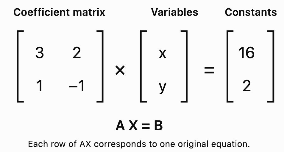
Consider the system:

3x + 2y = 16

x − y = 2

We can represent it using three matrices.

Coefficient matrix

The coefficient matrix contains the coefficients of the variables.

Variable matrix

The variable matrix contains the unknown quantities.

Constant matrix

The constant matrix contains the values on the right side of the equations.

The system can now be written as:

or:

Multiplying the matrices on the left gives:

This reproduces the original system.

Visualising the matrix representation

Important rules for constructing matrix equations

• Keep the variables in the same order in every equation.

• Include zero coefficients when a variable is missing.

• Place constants in the correct corresponding rows.

• Ensure the dimensions are compatible for multiplication.

Worked Example 1: Writing a System in Matrix Form

Write the following system in the form AX = B.

2x + 3y − z = 8

4x − y + 2z = 11

x + 5z = 7

Step 1: Identify the variables.

The variables are:

x, y, z

Step 2: Arrange the coefficients.

Notice that the third equation does not contain y.

Therefore, its y-coefficient is zero.

The coefficient matrix is:

Step 3: Construct the variable matrix.

Step 4: Construct the constant matrix.

Therefore:

The dimensions are:

A: 3 × 3

X: 3 × 1

B: 3 × 1

The multiplication is valid because:

(3 × 3)(3 × 1) = 3 × 1

Augmented Matrices

An augmented matrix combines the coefficient matrix and the constant matrix into one arrangement.

For the system:

3x + 2y = 16

x − y = 2

the augmented matrix is:

The vertical line separates the coefficients from the constants.

An augmented matrix is especially useful for solving systems through row operations.

Why augmented matrices are useful

They allow us to:

• Organise all the numerical information in one place.

• Perform elimination systematically.

• Solve systems with several variables.

• Identify systems with no solution.

• Identify systems with infinitely many solutions.

Solving Systems Using Gaussian Elimination

Gaussian elimination is a matrix method that uses elementary row operations to simplify a system.

The goal is to transform the augmented matrix into row echelon form, from which the variables can be found using back-substitution.

Elementary row operations

There are three allowed operations.

1. Interchange two rows.

2. Multiply a row by a nonzero number.

3. Add a multiple of one row to another row.

These operations preserve the solution set of the system.

Worked Example 2: Gaussian Elimination

Solve:

2x + y = 7

x − y = 2

Step 1: Construct the augmented matrix.

Step 2: Swap the rows.

This places a coefficient of 1 in the top-left position.

R₁ ↔ R₂

Step 3: Eliminate the x-coefficient in row 2.

R₂ → R₂ − 2R₁

Step 4: Solve for y.

The second row represents:

3y = 3

Therefore:

y = 1

Step 5: Substitute into the first equation.

x − y = 2

x − 1 = 2

x = 3

Therefore:

Verification

2(3) + 1 = 7

3 − 1 = 2

Both equations are satisfied.

Gauss–Jordan Elimination

Gauss–Jordan elimination extends Gaussian elimination by continuing the row operations until the coefficient portion is in reduced row echelon form.

For a system with a unique solution, the final matrix has the form:

The solution can be read directly from the final column.

Worked Example 3: Gauss–Jordan Elimination

Solve:

2x + y = 9

x + 2y = 6

Step 1: Write the augmented matrix.

Step 2: Swap the rows.

Step 3: Eliminate the 2 below the first pivot.

R₂ → R₂ − 2R₁

Step 4: Divide row 2 by −3.

R₂ → −(1/3)R₂

Step 5: Eliminate the 2 above the second pivot.

R₁ → R₁ − 2R₂

Therefore:

This method is particularly useful because it provides the solution without requiring a separate back-substitution stage.

Solving Systems Using Inverse Matrices

A system can be written as:

AX = B

If A is square and invertible:

This method is useful when the coefficient matrix has a nonzero determinant.

Worked Example 4: Solving with an Inverse Matrix

Solve:

3x + y = 11

2x + y = 8

Step 1: Write the system in matrix form.

Step 2: Calculate the determinant.

det(A) = 3(1) − 1(2)

= 1

The matrix is invertible.

Step 3: Find the inverse.

Step 4: Calculate X.

First element:

11 − 8 = 3

Second element:

−22 + 24 = 2

Therefore:

x = 3, y = 2

Verification

3(3) + 2 = 11

2(3) + 2 = 8

Both equations are satisfied.

Solving Systems Using Cramer's Rule

Cramer's Rule uses determinants to solve square systems with a nonzero coefficient determinant.

For:

ax + by = e

cx + dy = f

define:

If D ≠ 0:

Worked Example 5: Cramer's Rule

Solve:

2x + 3y = 13

x + y = 5

Step 1: Calculate D.

D = 2(1) − 3(1)

= −1

Step 2: Calculate Dₓ.

Dₓ = 13(1) − 3(5)

= −2

Step 3: Calculate Dᵧ.

Dᵧ = 2(5) − 13(1)

= −3

Step 4: Calculate x and y.

x = Dₓ/D = (−2)/(−1) = 2

y = Dᵧ/D = (−3)/(−1) = 3

Therefore:

Solving Systems with Three Unknowns

Matrix methods are particularly valuable for systems containing three or more variables.

Consider:

x + y + z = 6

2x − y + z = 3

x + 2y − z = 2

Worked Example 6: Three-Variable Gaussian Elimination

Step 1: Write the augmented matrix.

Step 2: Eliminate x from rows 2 and 3.

R₂ → R₂ − 2R₁

R₃ → R₃ − R₁

Step 3: Swap rows 2 and 3.

Step 4: Eliminate y from row 3.

R₃ → R₃ + 3R₂

Step 5: Solve for z.

−7z = −21

z = 3

Step 6: Solve for y.

From row 2:

y − 2z = −4

y − 6 = −4

y = 2

Step 7: Solve for x.

From row 1:

x + y + z = 6

x + 2 + 3 = 6

x = 1

Therefore:

Verification

First equation:

1 + 2 + 3 = 6

Second equation:

2(1) − 2 + 3 = 3

Third equation:

1 + 2(2) − 3 = 2

All three equations are satisfied.

Graphical Interpretation of Linear Systems

Every linear equation in two variables represents a straight line.

When two equations are considered together, their solutions correspond to the intersection points of the lines.

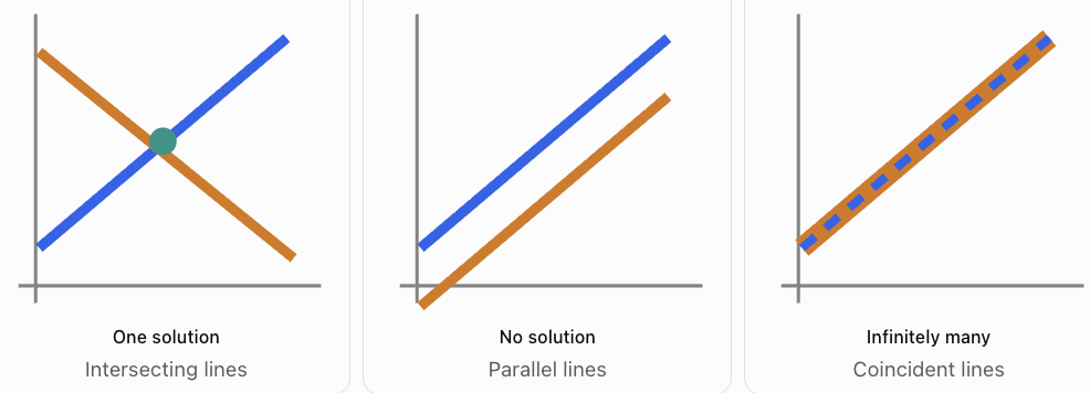
There are three main possibilities.

Case 1: One unique solution

Two nonparallel lines intersect at exactly one point.

For example:

y = 2x + 1

y = −x + 7

Set the equations equal:

2x + 1 = −x + 7

3x = 6

x = 2

Substitute:

y = 2(2) + 1 = 5

The intersection is:

(2, 5)

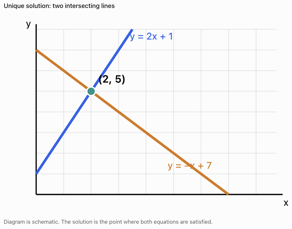
The coefficient determinant is nonzero, so the system has a unique solution.

Case 2: No solution

Consider:

y = 2x + 1

y = 2x − 3

Both lines have the same gradient but different y-intercepts.

They are parallel and never intersect.

Therefore:

The system has no solution.

The coefficient matrix has determinant zero.

Case 3: Infinitely many solutions

Consider:

2x + y = 6

4x + 2y = 12

The second equation is twice the first.

Both equations describe the same line.

Therefore:

The system has infinitely many solutions.

The coefficient matrix again has determinant zero.

Comparing the three cases

Matrix Interpretation of Different Solution Types

When using row reduction, the final augmented matrix reveals the nature of the system.

Unique solution

This represents:

x = 3

y = 2

There is one unique solution.

No solution

The second row represents:

0x + 0y = 3

or:

0 = 3

This is impossible.

Therefore, the system is inconsistent and has no solution.

Infinitely many solutions

The second row represents:

0 = 0

This provides no new restriction.

The first row gives:

x + 2y = 5

Let:

y = t

Then:

x = 5 − 2t

Therefore, the solutions can be written as:

(x, y) = (5 − 2t, t)

where t can be any real number.

This describes infinitely many solutions.

For a general system, the number of free variables determines the number of parameters needed to describe the solution set.

Systems of Three Equations: Graphical Interpretation

In three dimensions, a linear equation generally represents a plane rather than a line.

Three planes can:

• Intersect at one point.

• Share a common line.

• Coincide.

• Have no common intersection.

A unique solution corresponds to one point where all three planes meet.

A system with infinitely many solutions may have a common line or plane of solutions.

A system with no solution has no point satisfying all three equations simultaneously.

For a square 3 × 3 coefficient matrix:

• det(A) ≠ 0 guarantees one unique solution.

• det(A) = 0 means the system has no unique solution.

The second case must be investigated further to determine whether there are no solutions or infinitely many solutions.

Comparing Matrix and Algebraic Methods

Systems can be solved using several approaches.

Example: Comparing methods

Consider:

x + y = 7

x − y = 1

Algebraic elimination

Add the equations:

2x = 8

x = 4

Then:

y = 3

Matrix method

R₂ → R₂ − R₁

Therefore:

y = 3

x = 4

Both methods produce the same solution.

For a small system, algebraic elimination may be faster. For a system with many variables, matrix methods provide a more organised and scalable procedure.

Real-World Application 1: Ticket Sales

A school sells adult and student tickets for a concert.

Adult tickets cost $12.

Student tickets cost $7.

A total of 150 tickets are sold.

The total revenue is $1,350.

How many adult and student tickets were sold?

Step 1: Define variables

Let:

x = number of adult tickets

y = number of student tickets

Step 2: Construct equations

Total tickets:

x + y = 150

Total revenue:

12x + 7y = 1350

Step 3: Write the matrix equation

Step 4: Solve

The determinant is:

D = 1(7) − 1(12)

= −5

The inverse is:

Multiply:

First component:

(1050 − 1350)/(−5) = 60

Second component:

(−1800 + 1350)/(−5) = 90

Therefore:

60 adult tickets and 90 student tickets were sold.

Verification

60 + 90 = 150

12(60) + 7(90) = 720 + 630 = 1350

Both conditions are satisfied.

Real-World Application 2: Mixture Problems

A laboratory needs 20 litres of a 35% solution.

Two solutions are available:

• Solution A: 20% concentration.

• Solution B: 50% concentration.

How many litres of each solution should be mixed?

Step 1: Define variables

x = litres of 20% solution

y = litres of 50% solution

Step 2: Construct equations

Total volume:

x + y = 20

Amount of dissolved substance:

0.20x + 0.50y = 0.35(20)

Therefore:

0.20x + 0.50y = 7

Step 3: Matrix representation

Step 4: Solve by elimination

Multiply the first equation by 0.20:

0.20x + 0.20y = 4

Subtract from the concentration equation:

0.30y = 3

y = 10

Then:

x + 10 = 20

x = 10

Therefore:

10 litres of the 20% solution and 10 litres of the 50% solution are required.

This model assumes volumes are additive and the solutions mix uniformly.

Real-World Application 3: Production Planning

A workshop manufactures tables and chairs.

Each table requires:

• 4 hours of cutting.

• 2 hours of assembly.

Each chair requires:

• 2 hours of cutting.

• 3 hours of assembly.

The workshop has:

• 100 cutting hours.

• 90 assembly hours.

Determine how many tables and chairs can be manufactured if all available hours are used.

Let:

x = number of tables

y = number of chairs

The equations are:

4x + 2y = 100

2x + 3y = 90

The matrix equation is:

The determinant is:

D = 4(3) − 2(2)

= 8

The inverse is:

Calculate:

Therefore:

The workshop can manufacture 15 tables and 20 chairs.

Verification

Cutting:

4(15) + 2(20) = 100

Assembly:

2(15) + 3(20) = 90

The solution satisfies both resource constraints.

Real-World Application 4: Electrical Circuits

In electrical engineering, systems of linear equations are used to calculate unknown currents in circuits.

Kirchhoff's laws produce equations describing relationships between currents and voltages.

For example, suppose two unknown loop currents satisfy:

5I₁ − 2I₂ = 12

−2I₁ + 4I₂ = 6

The matrix equation is:

The determinant is:

D = 5(4) − (−2)(−2)

= 20 − 4

= 16

The inverse is:

Therefore:

Thus:

I₁ = 3.75 A

I₂ = 3.375 A

The currents satisfy the original equations.

This illustrates how matrix methods can solve systems arising in electrical engineering.

Choosing an Efficient Strategy

When solving a system, begin by examining its structure.

If the system has two equations with simple coefficients:

Substitution or elimination may be quickest.

If the system has three or more variables:

Gaussian elimination is often a good choice.

If the coefficient matrix is square and invertible:

Inverse matrices or Cramer's Rule are possible.

If you need to identify whether a system has no solution or infinitely many solutions:

Row reduction is particularly useful.

If a graphical interpretation is important:

Graph the equations to understand the solution geometrically.

If the system is large:

Computational linear algebra methods are usually more efficient than calculating a full inverse explicitly.

Common Mistakes

Mistake 1: Placing coefficients in the wrong columns

Always keep the variables in the same order.

Mistake 2: Forgetting zero coefficients

If an equation does not contain a variable, include a zero in its column.

Mistake 3: Mixing coefficients and constants

The augmented matrix must preserve the correct relationship between equations and constants.

Mistake 4: Performing row operations on only part of the augmented matrix

Every row operation must apply to the entire row, including the constant column.

Mistake 5: Making sign errors during elimination

Subtracting a negative number produces a positive result.

Mistake 6: Using inverse matrices when the determinant is zero

The inverse does not exist for a singular matrix.

Mistake 7: Assuming a zero determinant means no solution

A singular system may have no solutions or infinitely many solutions.

Mistake 8: Confusing Gaussian and Gauss–Jordan elimination

Gaussian elimination typically uses back-substitution; Gauss–Jordan elimination continues to reduced row echelon form.

Mistake 9: Interpreting every system as having one solution

Systems can have one, none, or infinitely many solutions.

Mistake 10: Forgetting to check answers

Substitute solutions into every original equation.

Mistake 11: Using graphing as though it always gives exact values

Graphical solutions may be approximate unless the intersection is known exactly.

Mistake 12: Ignoring real-world constraints

Negative quantities or fractional numbers of indivisible products may not be meaningful.

Key Terms

• Linear Equation: Equation involving variables only to the first power.

• System of Linear Equations: Collection of linear equations involving common variables.

• Simultaneous Solution: Values satisfying all equations in a system.

• Coefficient: Number multiplying a variable.

• Constant: Fixed numerical value.

• Coefficient Matrix: Matrix containing the coefficients of a linear system.

• Variable Matrix: Column matrix containing the unknown variables.

• Constant Matrix: Column matrix containing the right-hand-side values.

• Matrix Equation: Equation expressed using matrices.

• Augmented Matrix: Matrix combining coefficients and constants.

• Gaussian Elimination: Method using row operations to reach row echelon form.

• Gauss–Jordan Elimination: Method using row operations to reach reduced row echelon form.

• Elementary Row Operation: Allowed operation that preserves the solution set.

• Pivot: Leading nonzero entry used during row reduction.

• Row Echelon Form: Matrix form suitable for back-substitution.

• Reduced Row Echelon Form: Matrix form with leading ones and zeros elsewhere in pivot columns.

• Back-Substitution: Solving variables from the last equation upward.

• Inverse Matrix: Matrix reversing the multiplication effect of an invertible matrix.

• Determinant: Scalar value used to test invertibility of a square matrix.

• Cramer's Rule: Method solving square linear systems using determinants.

• Unique Solution: Exactly one solution satisfying the system.

• Inconsistent System: System with no solution.

• Dependent System: System containing redundant equations.

• Independent Equations: Equations contributing independent constraints.

• Singular Matrix: Square matrix with determinant zero.

• Free Variable: Variable that can take arbitrary values in a system with infinitely many solutions.

• Parameter: Symbol used to describe a family of solutions.

• Intersection Point: Point shared by two or more graphs.

• Parallel Lines: Lines in a plane that never intersect.

• Coincident Lines: Lines that occupy exactly the same position.

• Linear Model: Mathematical representation using linear relationships.

Key Takeaways

• A system of linear equations contains two or more equations involving common variables.

• A solution must satisfy every equation simultaneously.

• Systems can be represented compactly as AX = B.

• The coefficient matrix contains the variable coefficients.

• The augmented matrix combines coefficients and constants.

• Gaussian elimination uses row operations and back-substitution.

• Gauss–Jordan elimination reduces the system to a form where solutions can be read directly.

• Inverse matrices solve systems using X = A⁻¹B when A is invertible.

• Cramer's Rule uses determinants to solve square systems with nonzero determinants.

• A system can have one solution, no solution, or infinitely many solutions.

• In two dimensions, solutions correspond to intersections of lines.

• Parallel distinct lines produce no solution.

• Coincident lines produce infinitely many solutions.

• A nonzero determinant guarantees a unique solution for a square system.

• A zero determinant means a square system does not have a unique solution.

• Different solving methods are useful in different situations.

• Matrix methods are especially valuable for larger systems.

• Real-world applications include business, chemistry, engineering, and electrical circuits.

Check Your Understanding

Questions

Question 1: Matrix Representation

Write the system in matrix form:

2x + 3y = 12

4x − y = 5

Question 2: Augmented Matrix

Construct the augmented matrix for:

x + 2y = 7

3x − y = 8

Question 3: Missing Coefficient

Write the coefficient matrix for:

2x + 3z = 8

x + y − z = 4

3y + 2z = 9

Question 4: Gaussian Elimination

Solve:

x + y = 9

2x − y = 3

Question 5: Gauss–Jordan Elimination

Solve:

2x + y = 8

x + 3y = 9

Question 6: Inverse Matrix Method

Solve using an inverse matrix:

3x + y = 10

x + y = 6

Question 7: Cramer's Rule

Solve:

2x + y = 7

x − y = 2

Question 8: Graphical Interpretation

Determine the number of solutions:

y = 3x + 2

y = 3x − 5

Explain your reasoning.

Question 9: Infinitely Many Solutions

Determine the number of solutions:

2x + 4y = 12

x + 2y = 6

Question 10: Singular Matrix

Determine whether the coefficient matrix of:

3x + 6y = 9

x + 2y = 3

is singular.

Question 11: Three-Variable System

Solve:

x + y + z = 9

x − y + z = 3

2x + y − z = 3

Question 12: Ticket Sales

A cinema sells adult tickets for $15 and student tickets for $10.

A total of 120 tickets are sold.

Revenue is $1,500.

How many of each ticket were sold?

Question 13: Mixture Problem

A laboratory needs 30 litres of a 40% solution.

It has 20% and 50% solutions.

How many litres of each are required?

Question 14: Comparing Methods

Explain why Gaussian elimination may be preferable to graphing for a system with four unknown variables.

Question 15: Integrated Challenge

Consider:

2x + y = 11

3x − 2y = 4

a) Write the matrix equation AX = B.

b) Construct the augmented matrix.

c) Calculate det(A).

d) Solve the system using a matrix method.

e) Explain the graphical meaning of the solution.

f) Verify the solution.

Fully Worked Answers

Answer 1: Matrix Representation

System:

2x + 3y = 12

4x − y = 5

The coefficient matrix is:

The variable matrix is:

The constant matrix is:

Therefore:

Answer 2: Augmented Matrix

System:

x + 2y = 7

3x − y = 8

The augmented matrix is:

Answer 3: Missing Coefficient

System:

2x + 3z = 8

x + y − z = 4

3y + 2z = 9

The missing coefficients are zero.

Therefore:

Answer 4: Gaussian Elimination

System:

x + y = 9

2x − y = 3

Augmented matrix:

R₂ → R₂ − 2R₁

Therefore:

−3y = −15

y = 5

Substitute:

x + 5 = 9

x = 4

Answer: x = 4, y = 5

Answer 5: Gauss–Jordan Elimination

System:

2x + y = 8

x + 3y = 9

Augmented matrix:

Swap rows:

R₂ → R₂ − 2R₁

R₂ → −(1/5)R₂

R₁ → R₁ − 3R₂

Answer: x = 3, y = 2

Answer 6: Inverse Matrix Method

System:

3x + y = 10

x + y = 6

Coefficient matrix:

det(A) = 3(1) − 1(1)

= 2

Inverse:

Calculate:

Answer: x = 2, y = 4

Answer 7: Cramer's Rule

System:

2x + y = 7

x − y = 2

Calculate:

D = 2(−1) − 1(1)

= −3

Dₓ = 7(−1) − 1(2)

= −9

Dᵧ = 2(2) − 7(1)

= −3

Therefore:

x = Dₓ/D = (−9)/(−3) = 3

y = Dᵧ/D = (−3)/(−3) = 1

Answer: x = 3, y = 1

Answer 8: Graphical Interpretation

Equations:

y = 3x + 2

y = 3x − 5

Both lines have gradient 3.

However, their y-intercepts are different.

Therefore, they are distinct parallel lines.

Answer: No solution.

Answer 9: Infinitely Many Solutions

Equations:

2x + 4y = 12

x + 2y = 6

Multiply the second equation by 2:

2x + 4y = 12

This is identical to the first equation.

Therefore, both equations represent the same line.

Answer: Infinitely many solutions.

Answer 10: Singular Matrix

Coefficient matrix:

det(A) = 3(2) − 6(1)

= 6 − 6

= 0

Therefore:

Answer: The coefficient matrix is singular.

The equations are also consistent because the first is three times the second, so the system has infinitely many solutions.

Answer 11: Three-Variable System

System:

x + y + z = 9

x − y + z = 3

2x + y − z = 3

Subtract the second equation from the first:

2y = 6

y = 3

Substitute into the first equation:

x + z = 6

Substitute y = 3 into the third equation:

2x + 3 − z = 3

2x − z = 0

Therefore:

z = 2x

Substitute into x + z = 6:

x + 2x = 6

3x = 6

x = 2

Then:

z = 4

Answer: x = 2, y = 3, z = 4

Answer 12: Ticket Sales

Let:

x = adult tickets

y = student tickets

Equations:

x + y = 120

15x + 10y = 1500

Multiply the first equation by 10:

10x + 10y = 1200

Subtract:

5x = 300

x = 60

Then:

y = 120 − 60

y = 60

Answer: 60 adult tickets and 60 student tickets.

Verification:

15(60) + 10(60) = 1500

Answer 13: Mixture Problem

Let:

x = litres of 20% solution

y = litres of 50% solution

Total volume:

x + y = 30

Concentration equation:

0.20x + 0.50y = 0.40(30)

0.20x + 0.50y = 12

Multiply the volume equation by 0.20:

0.20x + 0.20y = 6

Subtract:

0.30y = 6

y = 20

Then:

x = 30 − 20

x = 10

Answer: 10 litres of 20% solution and 20 litres of 50% solution.

Answer 14: Comparing Methods

Gaussian elimination is preferable for a system with four unknowns because:

• It provides a systematic algebraic procedure.

• It can produce exact solutions.

• It avoids the difficulty of graphing equations in four dimensions.

• It can identify inconsistent or dependent systems.

• It extends naturally to larger systems.

Answer: Gaussian elimination is generally more practical and precise for systems involving several variables.

Answer 15: Integrated Challenge

System:

2x + y = 11

3x − 2y = 4

Part a: Matrix equation

Part b: Augmented matrix

Part c: Determinant

det(A) = 2(−2) − 1(3)

= −4 − 3

det(A) = −7

Since the determinant is nonzero, the system has one unique solution.

Part d: Solve using the inverse matrix

Calculate:

Therefore:

Part e: Graphical interpretation

The two lines intersect at exactly one point:

(26/7, 25/7)

This is the unique solution.

Part f: Verification

First equation:

2(26/7) + 25/7

= 52/7 + 25/7

= 77/7

= 11

Second equation:

3(26/7) − 2(25/7)

= 78/7 − 50/7

= 28/7

= 4

Both equations are satisfied.

Final Reflection

Systems of linear equations provide a mathematical framework for understanding relationships involving several unknown quantities.

Matrix notation allows us to represent these relationships efficiently and solve them using systematic procedures.

Gaussian elimination, Gauss–Jordan elimination, inverse matrices, and Cramer's Rule all provide ways to solve systems, but each method has different advantages.

Graphical interpretation helps us understand why systems may have one solution, no solution, or infinitely many solutions.

The greatest value of these methods becomes clear when they are applied to real-world situations. Business planning, scientific mixtures, engineering systems, and electrical circuits can all be represented using systems of linear equations.

The central idea is that matrix methods transform collections of linear equations into organised numerical structures that can be analysed, solved, and interpreted efficiently.