Introduction to Matrices
| Site: | Young Education |
| Cours: | Vectors and Matrices |
| Livre: | Introduction to Matrices |
| Imprimé par: | Guest user |
| Date: | lundi 9 novembre 2026, 16:38 |
1. Matrix Fundamentals
Learning outcomes
- I can define matrices and their dimensions.
- I can identify different types of matrices.
- I can represent data using matrices.
- I can interpret matrix notation.
- I can recognise practical uses of matrices.
Matrix Fundamentals
Introduction to Matrices
Matrices are mathematical structures used to organise, represent, and analyse information.
A matrix is a rectangular arrangement of numbers, variables, or mathematical expressions organised into rows and columns.
Matrices are particularly useful when working with large amounts of data, solving systems of equations, representing geometric transformations, and modelling relationships between quantities.
They are widely used in mathematics, engineering, computer science, economics, physics, statistics, and artificial intelligence.
For example, a school might record the test scores of several students across different subjects. Instead of writing each score separately, the information can be organised into a matrix.
Consider the following scores:
|
Student |
Mathematics |
Science |
English |
|---|---|---|---|
|
Alice |
85 |
90 |
78 |
|
Ben |
72 |
88 |
81 |
|
Chloe |
94 |
91 |
89 |
These scores can be represented by the matrix:
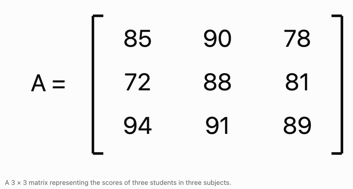
Each row represents one student.
Each column represents one subject.
Matrices allow this information to be stored and manipulated systematically.
Rows and Columns
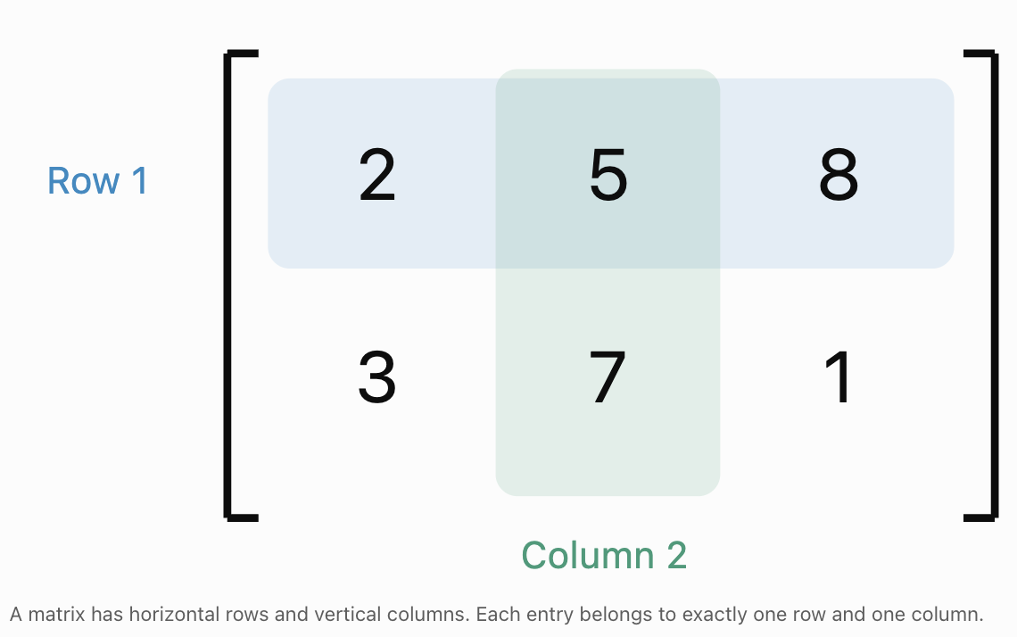
A matrix consists of horizontal rows and vertical columns.
-
A row is a horizontal arrangement of entries.
-
A column is a vertical arrangement of entries.
-
An element or entry is an individual value in a matrix.
Consider:
A = [[2, 5, 8], [3, 7, 1]]
The outer brackets enclose the matrix. Each inner bracket represents a row.
Identifying the Rows
Row 1:
[2, 5, 8]
Row 2:
[3, 7, 1]
Identifying the Columns
Column 1 contains 2 and 3.
Column 2 contains 5 and 7.
Column 3 contains 8 and 1.
Important Observation
The arrangement of values matters.
Changing the order of rows or columns may change the meaning of the data.
For example, swapping two student rows would change which student each set of scores represents.
Dimensions of a Matrix
The dimensions or order of a matrix describe its number of rows and columns.
The standard notation is:
m × n
where:
-
m = number of rows.
-
n = number of columns.
The number of rows is always written first.
Examples
|
Matrix |
Rows |
Columns |
Dimensions |
|---|---|---|---|
|
[[2, 4], [6, 8]] |
2 |
2 |
2 × 2 |
|
[[1, 3, 5]] |
1 |
3 |
1 × 3 |
|
[[4], [7], [9]] |
3 |
1 |
3 × 1 |
|
[[1, 2, 3], [4, 5, 6]] |
2 |
3 |
2 × 3 |
|
[[2, 0], [1, 4], [3, 5]] |
3 |
2 |
3 × 2 |
Worked Example: Determining Matrix Dimensions
Consider:
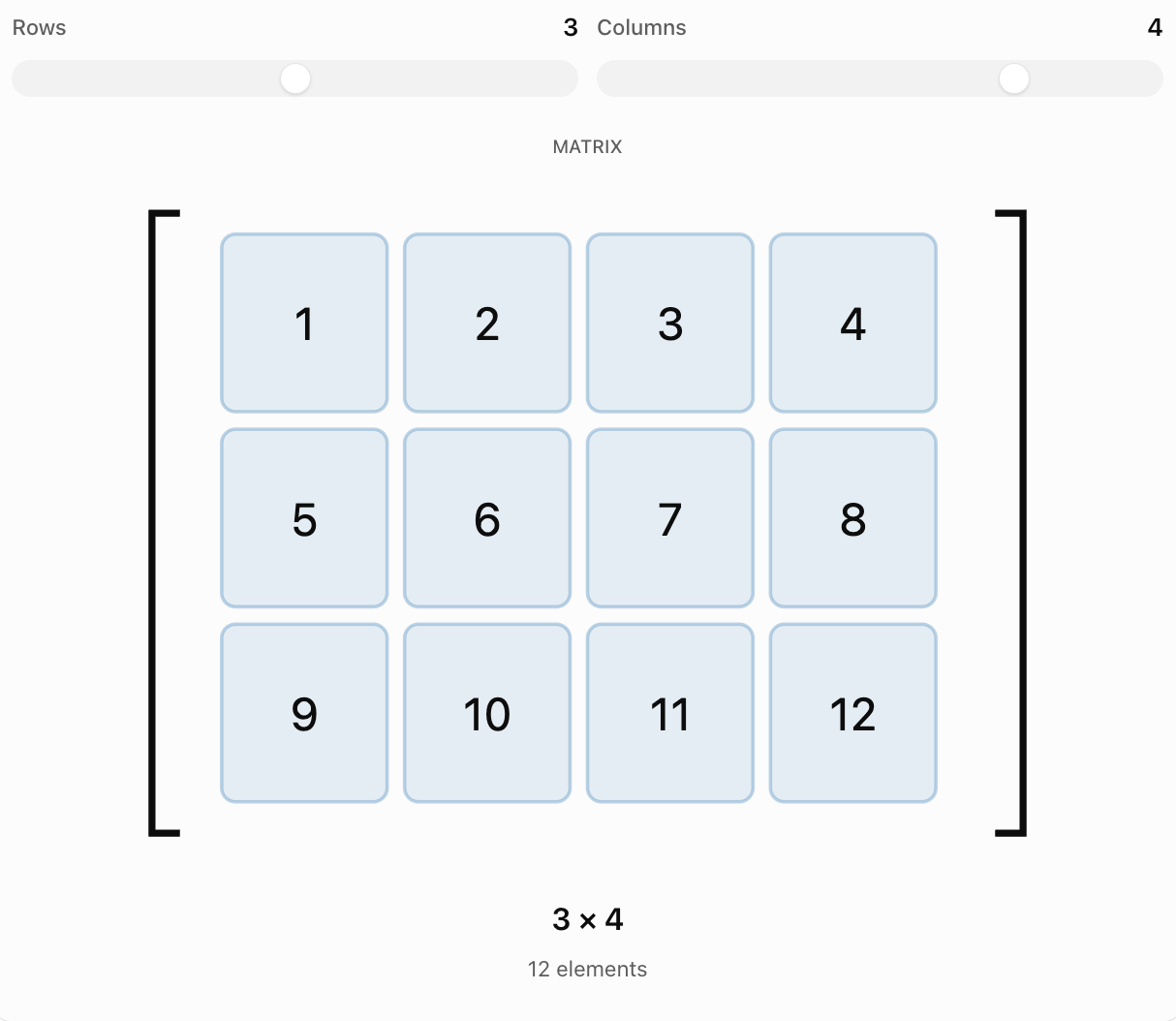
A = [[3, 7, 2, 5], [1, 4, 8, 6], [9, 0, 3, 2]]
Step 1: Count the rows
There are three rows.
Step 2: Count the columns
There are four columns.
Final Answer
A is a 3 × 4 matrix.
Number of Elements
A matrix with dimensions m × n contains:
Number of elements = m × n
For a 3 × 4 matrix:
3 × 4 = 12
Therefore, matrix A contains 12 elements.
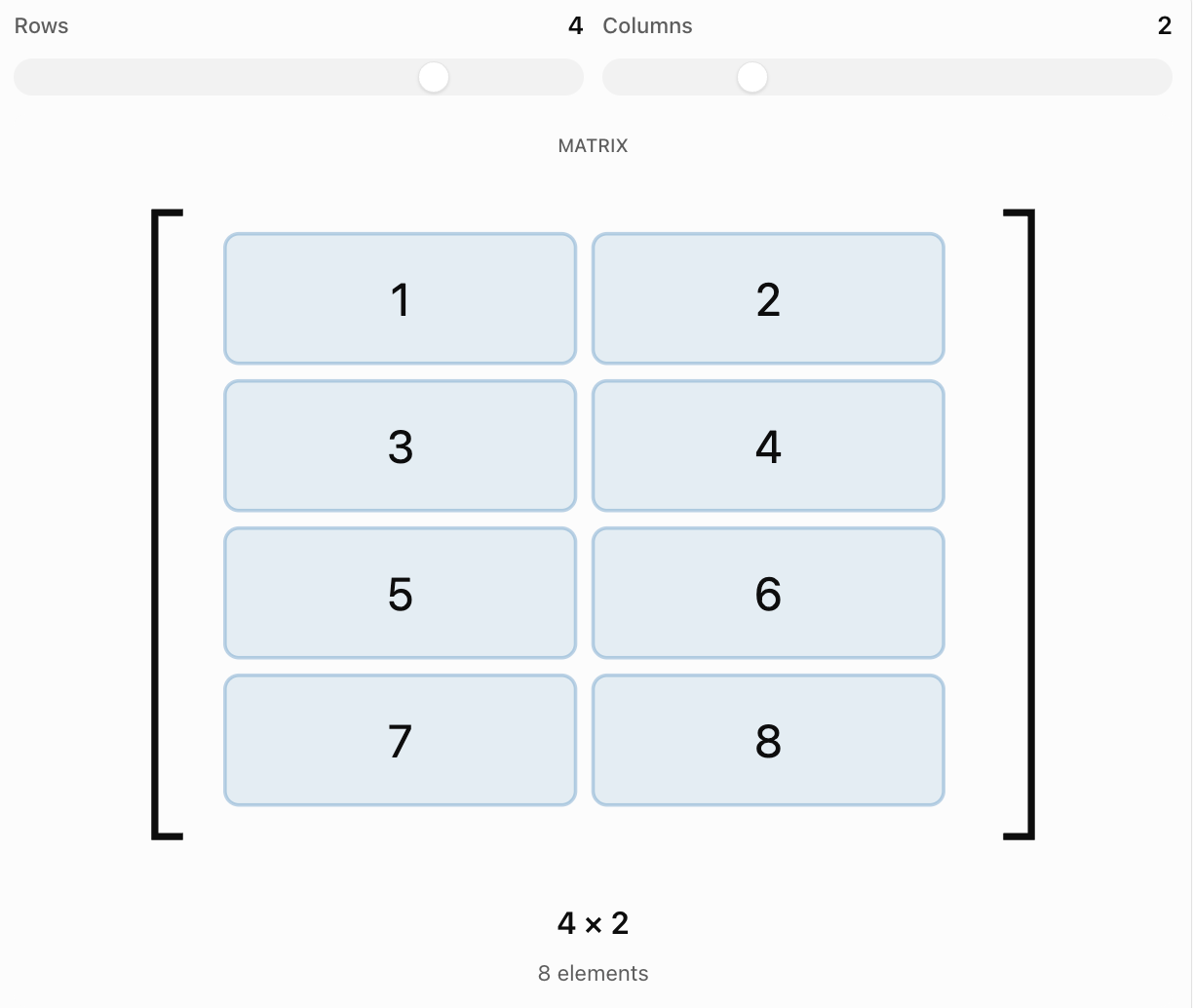
Explore Matrix Dimensions
Change the number of rows and columns to see how the dimensions and total number of elements change.
Matrix Notation
Matrices are usually represented by capital letters:
A, B, C, M, X
Individual entries are represented by lowercase letters with subscripts.
For a matrix A, an entry is written:
aᵢⱼ
where:
-
i identifies the row.
-
j identifies the column.
The first subscript always refers to the row.
The second subscript refers to the column.
For example:
a₂₃
means the element in row 2, column 3.
Worked Example: Reading Matrix Entries
Consider:
A = [[4, 7, 2], [9, 1, 5], [6, 8, 3]]
Find:
-
a₁₂
-
a₂₃
-
a₃₁
-
a₃₃
Step 1: Find a₁₂
Row 1, column 2 contains 7.
a₁₂ = 7
Step 2: Find a₂₃
Row 2, column 3 contains 5.
a₂₃ = 5
Step 3: Find a₃₁
Row 3, column 1 contains 6.
a₃₁ = 6
Step 4: Find a₃₃
Row 3, column 3 contains 3.
a₃₃ = 3
Important Principle
Matrix subscripts are read row first, column second.
General Matrix Representation
A matrix with m rows and n columns can be written:
A = [aᵢⱼ], where i = 1, 2, ..., m and j = 1, 2, ..., n.
For a 2 × 3 matrix:
A = [[a₁₁, a₁₂, a₁₃], [a₂₁, a₂₂, a₂₃]]
The entries may be:
-
Numbers.
-
Variables.
-
Algebraic expressions.
-
Measurements.
-
Data values.
Example: A Matrix Containing Variables
B = [[x, 2y], [3x, y + 1]]
This is a 2 × 2 matrix.
If x = 2 and y = 3:
B = [[2, 6], [6, 4]]
Matrices do not need to contain only fixed numerical values.
Types of Matrices
Matrices can be classified according to their dimensions and the arrangement of their entries.
Row Matrix
A row matrix contains exactly one row.
Example:
A = [[3, 5, 7, 9]]
Dimensions:
1 × 4
Row matrices are useful for representing a single set of related values.
For example, one student's scores across four subjects.
Column Matrix
A column matrix contains exactly one column.
Example:
B = [[2], [4], [6]]
Dimensions:
3 × 1
Column matrices are commonly used to represent vectors.
For example, the three-dimensional position vector (2, 4, 6) can be represented as a column matrix.
Rectangular Matrix
A rectangular matrix has a different number of rows and columns.
Example:
C = [[1, 2, 3], [4, 5, 6]]
Dimensions:
2 × 3
Rectangular matrices are frequently used to organise data tables.
Square Matrix
A square matrix has the same number of rows and columns.
Example:
D = [[2, 5], [7, 3]]
Dimensions:
2 × 2
Another example:
E = [[1, 2, 3], [4, 5, 6], [7, 8, 9]]
Dimensions:
3 × 3
Square matrices are particularly important in systems of equations, transformations, and advanced matrix operations.
Zero Matrix
A zero matrix contains only zeros.
Example:
O = [[0, 0, 0], [0, 0, 0]]
Dimensions:
2 × 3
Another example:
O = [[0, 0], [0, 0]]
Dimensions:
2 × 2
Important Properties
-
Every entry is zero.
-
Zero matrices can have different dimensions.
-
A zero matrix does not have to be square.
The zero matrix plays a role similar to the number zero in ordinary arithmetic.
For matrix addition, it acts as an additive identity when its dimensions match those of the other matrix.
Identity Matrix
An identity matrix is a square matrix with:
-
Ones along the main diagonal.
-
Zeros everywhere else.
The main diagonal extends from the upper-left corner to the lower-right corner.
Identity Matrix of Order 2
I₂ = [[1, 0], [0, 1]]
Identity Matrix of Order 3
I₃ = [[1, 0, 0], [0, 1, 0], [0, 0, 1]]
Important Property
When a matrix A is multiplied by a compatible identity matrix, A remains unchanged.
For a 2 × 2 matrix:
AI₂ = I₂A = A
This is similar to multiplying a number by 1.
Why Identity Matrices Matter
Identity matrices are used in:
-
Matrix multiplication.
-
Matrix inverses.
-
Coordinate transformations.
-
Systems of linear equations.
-
Computer graphics.
Diagonal Matrix
A diagonal matrix is a square matrix in which all entries outside the main diagonal are zero.
Example:
D = [[4, 0, 0], [0, 7, 0], [0, 0, 2]]
The diagonal entries are:
4, 7, 2
A diagonal matrix may contain zeros on its main diagonal.
Important Observation
Every identity matrix is a diagonal matrix.
However, not every diagonal matrix is an identity matrix.
Scalar Matrix
A scalar matrix is a diagonal matrix in which every entry on the main diagonal has the same value.
Example:
S = [[5, 0, 0], [0, 5, 0], [0, 0, 5]]
This can also be written:
S = 5I₃
A scalar matrix is useful for representing uniform scaling.
For example, multiplying coordinate vectors by 5 enlarges them by a factor of 5 relative to the origin.
Upper and Lower Triangular Matrices
Triangular matrices are square matrices with zeros on one side of the main diagonal.
Upper Triangular Matrix
All entries below the main diagonal are zero.
U = [[2, 4, 6], [0, 3, 5], [0, 0, 7]]
Lower Triangular Matrix
All entries above the main diagonal are zero.
L = [[2, 0, 0], [4, 3, 0], [6, 5, 7]]
Triangular matrices are important in numerical methods and solving systems of linear equations.
Symmetric Matrix
A symmetric matrix is a square matrix whose entries are mirrored across the main diagonal.
Example:
A = [[2, 5, 7], [5, 3, 4], [7, 4, 6]]
Notice:
a₁₂ = a₂₁ = 5
a₁₃ = a₃₁ = 7
a₂₃ = a₃₂ = 4
A symmetric matrix satisfies:
Aᵀ = A
where Aᵀ represents the transpose of A.
Symmetric matrices appear in statistics, physics, optimisation, and engineering.
Comparing Matrix Types
|
Matrix type |
Main characteristic |
Example |
|---|---|---|
|
Row |
One row |
[[2, 4, 6]] |
|
Column |
One column |
[[2], [4], [6]] |
|
Rectangular |
Different numbers of rows and columns |
[[1, 2, 3], [4, 5, 6]] |
|
Square |
Equal numbers of rows and columns |
[[1, 2], [3, 4]] |
|
Zero |
All entries are zero |
[[0, 0], [0, 0]] |
|
Identity |
Ones on main diagonal, zeros elsewhere |
[[1, 0], [0, 1]] |
|
Diagonal |
Zeros outside main diagonal |
[[3, 0], [0, 7]] |
|
Scalar |
Equal diagonal entries, zeros elsewhere |
[[5, 0], [0, 5]] |
|
Upper triangular |
Zeros below main diagonal |
[[2, 3], [0, 4]] |
|
Lower triangular |
Zeros above main diagonal |
[[2, 0], [3, 4]] |
|
Symmetric |
Mirrored across main diagonal |
[[2, 5], [5, 3]] |
A matrix may belong to more than one category.
For example, an identity matrix is also square, diagonal, scalar, upper triangular, lower triangular, and symmetric.
Representing Data Using Matrices
One of the most common applications of matrices is organising data.
Rows and columns allow related values to be stored in a consistent structure.
Example: School Attendance
A school records the number of students present in three classes over four days.
|
Class |
Monday |
Tuesday |
Wednesday |
Thursday |
|---|---|---|---|---|
|
Class A |
24 |
23 |
25 |
24 |
|
Class B |
21 |
22 |
20 |
23 |
|
Class C |
26 |
25 |
24 |
26 |
The data can be represented as:
A = [[24, 23, 25, 24], [21, 22, 20, 23], [26, 25, 24, 26]]
Interpretation
-
The matrix has three rows.
-
The matrix has four columns.
-
Its dimensions are 3 × 4.
-
Each row represents a class.
-
Each column represents a day.
Worked Example: Reading Attendance Data
What does a₂₃ represent?
Row 2 corresponds to Class B.
Column 3 corresponds to Wednesday.
Therefore:
a₂₃ = 20
This means 20 students were present in Class B on Wednesday.
Why Matrix Labels Matter
The numbers alone do not explain what they represent.
A matrix becomes meaningful when the rows, columns, and units are clearly identified.
Worked Example: Organising Sales Data
A company sells three products in two stores.
The number of products sold during one week is:
|
Store |
Product A |
Product B |
Product C |
|---|---|---|---|
|
Store 1 |
40 |
25 |
30 |
|
Store 2 |
35 |
45 |
20 |
Represent this information as a matrix.
Step 1: Identify the rows
There are two stores.
Therefore, the matrix needs two rows.
Step 2: Identify the columns
There are three products.
Therefore, the matrix needs three columns.
Step 3: Write the matrix
S = [[40, 25, 30], [35, 45, 20]]
Final Answer
The sales matrix has dimensions:
2 × 3
Interpreting Entries
s₁₂ = 25 means Store 1 sold 25 units of Product B.
s₂₃ = 20 means Store 2 sold 20 units of Product C.
Extending the Example
The total number of products sold by Store 1 is:
40 + 25 + 30 = 95
The total number of products sold by Store 2 is:
35 + 45 + 20 = 100
Matrices make it easier to organise information for later calculations.
Representing Images Using Matrices
Digital images can be represented using matrices.
Each pixel has a numerical value describing its colour or brightness.
For a grayscale image:
-
0 commonly represents black.
-
255 commonly represents white.
-
Intermediate values represent shades of gray.
Consider:
P = [[0, 64, 128], [64, 128, 192], [128, 192, 255]]
This matrix represents a simple 3 × 3 grayscale image.
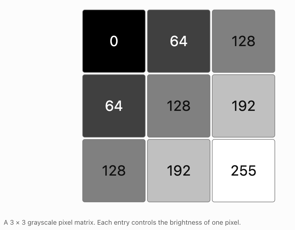
Interpretation
-
The top-left pixel has brightness 0.
-
The centre pixel has brightness 128.
-
The bottom-right pixel has brightness 255.
Colour Images
Colour images often use separate matrices for red, green, and blue intensity values.
This is the basis of the RGB colour model.
Practical Uses
Image matrices are used in:
-
Photography.
-
Medical imaging.
-
Computer vision.
-
Video processing.
-
Facial recognition systems.
-
Satellite imagery.
-
Artificial intelligence.


Representing Systems of Equations
Matrices provide an organised way to represent systems of linear equations.
Consider:
2x + 3y = 7
4x − y = 5
The coefficients can be arranged into the matrix:
A = [[2, 3], [4, −1]]
The variables can be represented as a column matrix:
X = [[x], [y]]
The constants can be represented as:
B = [[7], [5]]
The system can then be written:
AX = B
This is called the matrix form of a system of linear equations.
Why This Is Useful
Matrix methods allow large systems of equations to be solved systematically.
They are especially useful when systems contain many variables and equations.
For example, engineers may use matrices to solve systems describing forces, electrical circuits, or structural stresses.
Matrices in Geometric Transformations
Matrices can describe geometric transformations such as:
-
Rotations.
-
Reflections.
-
Dilations.
-
Combinations of transformations.
Example: Rotation Matrix
A 90° counterclockwise rotation about the origin can be represented by:
R = [[0, −1], [1, 0]]
This matrix transforms points according to:
(x, y) → (−y, x)
For example:
P = (3, 2)
After rotation:
P′ = (−2, 3)
Example: Dilation Matrix
A dilation with scale factor 2 can be represented by:
D = [[2, 0], [0, 2]]
This produces:
(x, y) → (2x, 2y)
For example:
P = (3, 2)
After dilation:
P′ = (6, 4)

Important Observation
Matrix transformations are fundamental in computer graphics and engineering design.
They allow geometric objects to be transformed efficiently using mathematical operations.
Matrices in Economics and Business
Businesses use matrices to organise and analyse numerical information.
Examples include:
-
Sales figures.
-
Production quantities.
-
Inventory levels.
-
Employee schedules.
-
Transportation costs.
-
Financial models.
Worked Example: Production Data
A factory produces three products during two shifts.
|
Shift |
Product A |
Product B |
Product C |
|---|---|---|---|
|
Morning |
120 |
90 |
60 |
|
Evening |
100 |
110 |
80 |
The production matrix is:
P = [[120, 90, 60], [100, 110, 80]]
Questions
How many units of Product B are produced during the evening shift?
p₂₂ = 110
How many units of Product C are produced during the morning shift?
p₁₃ = 60
What are the dimensions of P?
2 × 3
Interpretation
The matrix provides a compact representation of production data.
It can later be used to calculate totals, costs, revenue, and resource requirements.
Matrices in Science and Engineering
Matrices are used extensively in scientific and engineering calculations.
Physics
Matrices can represent:
-
Rotations.
-
Coordinate transformations.
-
Systems of forces.
-
Electrical circuits.
-
Quantum mechanical operations.
Engineering
Matrices are used to model:
-
Structural forces.
-
Mechanical systems.
-
Electrical networks.
-
Robotics.
-
Control systems.
-
Three-dimensional transformations.
Chemistry
Matrices can help organise:
-
Chemical reaction coefficients.
-
Stoichiometric relationships.
-
Experimental measurements.
-
Reaction networks.
Biology
Matrices are used in:
-
Population models.
-
Genetics.
-
Ecological interactions.
-
Biological networks.
-
Medical imaging.


Matrices in Networks
Matrices can represent relationships between connected objects.
For example, consider three cities:
A, B, and C.
Suppose:
-
A is connected to B.
-
B is connected to C.
-
A is not directly connected to C.
This information can be represented using an adjacency matrix.
M = [[0, 1, 0], [1, 0, 1], [0, 1, 0]]
Here:
-
1 indicates a direct connection.
-
0 indicates no direct connection.
The diagonal entries are zero because the model does not include connections from a city to itself.
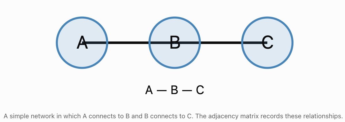
Interpreting the Matrix
m₁₂ = 1 means A is directly connected to B.
m₁₃ = 0 means A is not directly connected to C.
m₂₃ = 1 means B is directly connected to C.
Practical Uses
Adjacency matrices are used in:
-
Transportation networks.
-
Computer networks.
-
Social networks.
-
Communication systems.
-
Graph theory.
-
Route planning.
Matrices in Artificial Intelligence
Modern artificial intelligence relies heavily on matrices.
Data, model parameters, and calculations are often represented using arrays of numbers.
For example, a simple dataset containing four observations and three measured features can be represented by a 4 × 3 matrix.
X = [[2, 5, 1], [3, 4, 2], [6, 7, 3], [5, 8, 4]]
Each row represents one observation.
Each column represents one feature.
Why Matrices Are Useful in AI
Matrices allow computers to perform many calculations efficiently.
They are used in:
-
Machine learning.
-
Neural networks.
-
Image recognition.
-
Language processing.
-
Recommendation systems.
-
Data classification.

Important Observation
The mathematical operations performed on matrices allow AI systems to process large quantities of information.
Understanding matrix fundamentals is an important foundation for studying machine learning and advanced computing.
Matrix Equality
Two matrices are equal when:
-
They have the same dimensions.
-
Their corresponding entries are equal.
Consider:
A = [[2, 5], [7, 3]]
B = [[2, 5], [7, 3]]
Since every corresponding entry is equal:
A = B
However:
C = [[2, 7], [5, 3]]
Although C contains the same four numbers, they are arranged differently.
Therefore:
A ≠ C
Worked Example: Finding Unknown Entries
Suppose:
A = [[x, 4], [7, y]]
and:
B = [[3, 4], [7, 9]]
If A = B, find x and y.
Corresponding entries must be equal.
Therefore:
x = 3
y = 9
Final Answer
x = 3 and y = 9
The Transpose of a Matrix
The transpose of a matrix is obtained by interchanging its rows and columns.
The transpose of A is written:
Aᵀ
For example:
A = [[1, 2, 3], [4, 5, 6]]
The rows of A become the columns of Aᵀ.
Therefore:
Aᵀ = [[1, 4], [2, 5], [3, 6]]
Dimensions
Original matrix:
2 × 3
Transpose:
3 × 2
Important Principle
If A has dimensions m × n, then Aᵀ has dimensions n × m.
Practical Uses
Transposes are useful in:
-
Data analysis.
-
Matrix multiplication.
-
Statistics.
-
Engineering.
-
Machine learning.
Matrix Notation in Mathematical Models
Matrices can represent mathematical relationships in a compact form.
For example, consider the equations:
x + 2y = 8
3x + 4y = 18
The coefficient matrix is:
A = [[1, 2], [3, 4]]
The variable matrix is:
X = [[x], [y]]
The constant matrix is:
B = [[8], [18]]
The system is written:
AX = B
Interpretation
The matrix A stores the coefficients.
The matrix X stores the unknown variables.
The matrix B stores the constants.
This notation becomes especially valuable when working with larger systems.
Common Mistakes
Confusing rows and columns
Rows are horizontal, while columns are vertical.
Writing dimensions in the wrong order
Matrix dimensions are written rows × columns, not columns × rows.
Misreading matrix subscripts
The first subscript indicates the row, and the second indicates the column.
Assuming all matrices are square
Matrices can have different numbers of rows and columns.
Assuming a zero matrix must be square
Zero matrices can have any dimensions.
Confusing a zero matrix with an identity matrix
A zero matrix contains only zeros, while an identity matrix contains ones along the main diagonal.
Assuming all diagonal matrices are identity matrices
Diagonal matrices may have values other than 1 on the main diagonal.
Confusing row matrices and column matrices
A row matrix has one row, while a column matrix has one column.
Ignoring the order of entries
The positions of entries are important.
Assuming matrices with the same values are equal
Corresponding entries must appear in the same positions.
Forgetting that matrices may contain variables
Matrix entries can be numbers, variables, or expressions.
Misinterpreting matrix data
Rows and columns must be associated with their correct labels.
Confusing matrix dimensions with the number of elements
A 3 × 4 matrix has dimensions 3 × 4 but contains 12 elements.
Confusing a matrix with its transpose
Transposition interchanges rows and columns.
Assuming matrix notation is only used in mathematics
Matrices are widely used in science, engineering, economics, computing, and data analysis.
Key Terms
-
Matrix: A rectangular arrangement of numbers, variables, or expressions organised into rows and columns.
-
Row: A horizontal arrangement of entries in a matrix.
-
Column: A vertical arrangement of entries in a matrix.
-
Element: An individual value or expression within a matrix.
-
Entry: Another name for a matrix element.
-
Dimensions: The number of rows and columns in a matrix.
-
Order of a Matrix: Another term for its dimensions.
-
m × n Matrix: A matrix with m rows and n columns.
-
Matrix Notation: The mathematical symbols used to represent matrices and their entries.
-
Subscript: A small index identifying the position of an entry.
-
Row Matrix: A matrix containing exactly one row.
-
Column Matrix: A matrix containing exactly one column.
-
Rectangular Matrix: A matrix with different numbers of rows and columns.
-
Square Matrix: A matrix with equal numbers of rows and columns.
-
Zero Matrix: A matrix in which every entry is zero.
-
Identity Matrix: A square matrix with ones on the main diagonal and zeros elsewhere.
-
Diagonal Matrix: A square matrix with zeros outside the main diagonal.
-
Scalar Matrix: A diagonal matrix with equal diagonal entries.
-
Upper Triangular Matrix: A square matrix with zeros below the main diagonal.
-
Lower Triangular Matrix: A square matrix with zeros above the main diagonal.
-
Symmetric Matrix: A square matrix equal to its transpose.
-
Main Diagonal: The entries extending from the upper-left corner to the lower-right corner of a matrix.
-
Transpose: A matrix obtained by interchanging rows and columns.
-
Matrix Equality: A relationship in which matrices have identical dimensions and corresponding entries.
-
Coefficient Matrix: A matrix containing the coefficients of variables in a system of equations.
-
Column Vector: A vector represented as a matrix with one column.
-
Transformation Matrix: A matrix used to represent a geometric transformation.
-
Adjacency Matrix: A matrix describing connections between objects in a network.
-
Data Matrix: A matrix used to organise observations or measurements.
-
Pixel Matrix: A matrix representing image brightness or colour information.
-
Matrix Multiplication: An operation combining matrices according to row-and-column calculations.
-
Linear System: A collection of linear equations involving common variables.
-
Mathematical Model: A mathematical representation of a real-world situation.
-
RGB Colour Model: A system representing colours using red, green, and blue intensity values.
-
Machine Learning: A field of computing that develops systems capable of learning patterns from data.
Key Takeaways
-
A matrix is a rectangular arrangement of entries organised into rows and columns.
-
Matrix dimensions are written as rows × columns.
-
An m × n matrix contains m rows and n columns.
-
The total number of entries in a matrix is m × n.
-
Matrix entries are identified using row and column subscripts.
-
The notation aᵢⱼ represents the entry in row i, column j.
-
Matrices may contain numbers, variables, or expressions.
-
Row matrices contain one row.
-
Column matrices contain one column.
-
Rectangular matrices have different numbers of rows and columns.
-
Square matrices have equal numbers of rows and columns.
-
Zero matrices contain only zeros.
-
Identity matrices contain ones on the main diagonal and zeros elsewhere.
-
Diagonal matrices contain zeros outside the main diagonal.
-
Scalar matrices have equal diagonal entries.
-
Triangular matrices contain zeros above or below the main diagonal.
-
Symmetric matrices are mirrored across the main diagonal.
-
Two matrices are equal only when their dimensions and corresponding entries match.
-
Transposing a matrix interchanges its rows and columns.
-
Matrices can organise and represent data efficiently.
-
Matrices are used to represent systems of equations and geometric transformations.
-
Matrices are important in science, engineering, economics, statistics, computer graphics, and artificial intelligence.
-
Understanding matrix structure, notation, dimensions, and types provides the foundation for more advanced matrix operations and applications.
Check Your Understanding
Recall and Understanding
-
Define a matrix and explain the difference between a row and a column.
-
What are the dimensions of a matrix containing four rows and three columns?
-
Explain the meaning of the notation a₂₃.
-
Describe the difference between a row matrix and a column matrix.
-
Explain how an identity matrix differs from a zero matrix.
Application
6. Determine the dimensions and number of elements in:
A = [[2, 4, 6], [1, 3, 5], [7, 8, 9], [0, 2, 4]]
7. Given:
B = [[5, 8, 2], [3, 7, 9], [4, 1, 6]]
Find b₁₃, b₂₂, b₃₁, and b₃₃.
8. Write a 2 × 3 matrix representing the following sales data:
Store A sold 12 books, 8 pens, and 5 notebooks.
Store B sold 9 books, 15 pens, and 7 notebooks.
-
Write the 3 × 3 identity matrix.
-
Find the transpose of:
C = [[1, 4, 7], [2, 5, 8]]
Analysis and Challenge
11. Classify the following matrix as many ways as possible:
D = [[4, 0, 0], [0, 4, 0], [0, 0, 4]]
12. Determine whether the following matrices are equal:
A = [[2, 5], [7, 3]]
B = [[2, 7], [5, 3]]
Explain your reasoning.
13. If:
A = [[x, 3], [5, y]]
and:
B = [[7, 3], [5, 2]]
find x and y, given that A = B.
14. A digital grayscale image is represented by a 5 × 8 matrix. How many pixels does it contain? Explain what each entry represents.
15. Three towns are connected as follows: A is connected to B, A is connected to C, and B is not directly connected to C. Construct a 3 × 3 adjacency matrix for this undirected network, assuming no town is connected to itself.
Final Summary
Matrices are mathematical structures used to organise information into rows and columns.
Their dimensions describe the number of rows and columns, while matrix notation allows individual entries to be identified precisely.
Different matrix types have special properties. Row matrices, column matrices, square matrices, zero matrices, identity matrices, diagonal matrices, triangular matrices, and symmetric matrices each play important roles in mathematics.
Matrices are especially valuable because they provide a compact and systematic way to represent information.
They are used to organise data, describe systems of equations, represent geometric transformations, model networks, and perform calculations in science, engineering, economics, and computer science.
Understanding matrix fundamentals prepares students for more advanced topics such as matrix addition, scalar multiplication, matrix multiplication, determinants, inverses, systems of linear equations, and transformations.
The central principle is that matrices provide an organised mathematical language for representing and analysing relationships between quantities, making them essential tools in both pure mathematics and real-world applications.
2. Matrix Operations
Learning outcomes
- I can add and subtract matrices.
- I can multiply matrices by scalars.
- I can multiply compatible matrices.
- I can identify when matrix operations are possible.
- I can solve problems involving matrix operations.
Introduction
Mathematics often involves organising information and performing calculations with many values at once. A shop may track sales of several products across different months, a scientist may record measurements from multiple experiments, and a computer may transform thousands of points in a digital image.
One mathematical tool used in these situations is the matrix.
A matrix is a rectangular arrangement of numbers, symbols, or expressions organised into rows and columns. Matrices allow us to represent data efficiently and perform calculations systematically.
For example, consider the sales of three products in two stores:
|
Store |
Pens |
Pencils |
Notebooks |
|---|---|---|---|
|
Store A |
20 |
35 |
15 |
|
Store B |
30 |
25 |
18 |
We can represent this information using a matrix:
If we have another matrix representing sales during a second week, we can add the matrices to find total sales.
We can also multiply matrices by numbers, combine different matrices through multiplication, and use matrices to solve real-world problems involving transformations, production, finance, and scientific measurements.
However, matrix operations follow specific rules. Unlike ordinary numbers, matrices cannot always be added or multiplied, and the order of multiplication can change the result.
Understanding these rules is essential for working confidently with matrices.
What Is a Matrix?
A matrix is a rectangular array of elements arranged in rows and columns.
Matrices are usually represented using capital letters such as A, B, and C.
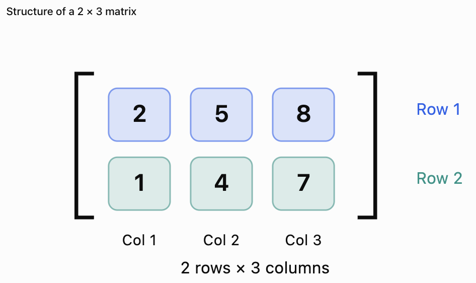
For example:
This matrix contains:
-
2 rows
-
3 columns
-
6 elements
The order, or dimensions, of the matrix are:
2 × 3
The number of rows is always written first, followed by the number of columns.
Identifying rows and columns
Matrix notation
An element of a matrix can be identified using two subscripts.
For example:
aᵢⱼ
where:
-
i identifies the row.
-
j identifies the column.
For the matrix A above:
a₁₁ = 2
a₁₂ = 5
a₁₃ = 8
a₂₁ = 1
a₂₂ = 4
a₂₃ = 7
Notice that a₂₃ means the element in row 2, column 3.
It does not mean row 3, column 2.
Types of Matrices
Matrices can be classified according to their dimensions and properties.
Row matrix
A matrix containing one row.
Order: 1 × 3
Column matrix
A matrix containing one column.
Order: 3 × 1
Square matrix
A matrix with the same number of rows and columns.
Order: 2 × 2
Zero matrix
A matrix in which every element is zero.
Identity matrix
A square matrix with 1 along the main diagonal and 0 everywhere else.
For example:
The identity matrix has an important role in matrix multiplication.
For any compatible matrix A:
AI = A and IA = A
The identity matrices used on the two sides may have different orders when A is rectangular.
Adding Matrices
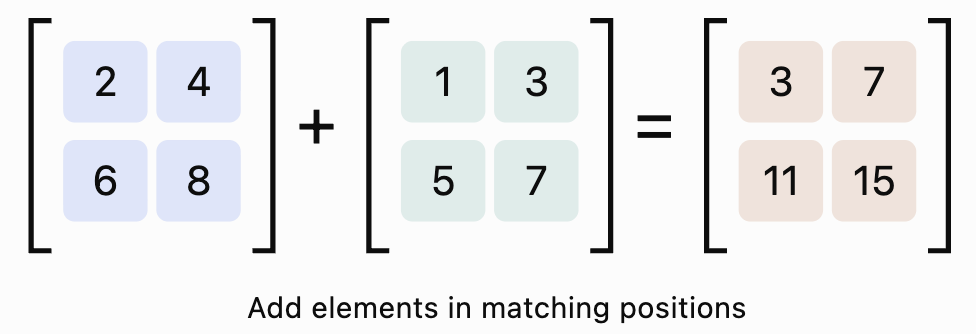
Matrix addition combines corresponding elements from two matrices.
Two matrices can be added only when they have the same dimensions.
For example:
Add corresponding elements:
Therefore:
Visualising matrix addition
General rule
If A and B are both m × n matrices:
(A + B)ᵢⱼ = aᵢⱼ + bᵢⱼ
The result is also an m × n matrix.
Worked Example 1: Adding 2 × 3 Matrices
Given:
Calculate A + B.
Step 1: Check the dimensions.
Both matrices are 2 × 3.
Addition is possible.
Step 2: Add corresponding elements.
Step 3: Simplify.
Properties of Matrix Addition
Matrix addition has several useful properties.
Commutative property
A + B = B + A
The order of addition does not affect the result.
Associative property
(A + B) + C = A + (B + C)
Matrices can be grouped differently when adding three or more matrices.
Additive identity
A + O = A
Adding a zero matrix of the same dimensions does not change a matrix.
Additive inverse
For every matrix A, there is a matrix −A such that:
A + (−A) = O
The additive inverse is formed by changing the sign of every element.
For example:
Then:
Subtracting Matrices
Matrix subtraction follows the same dimensional rule as addition.
Two matrices can be subtracted only if they have the same dimensions.
Subtract corresponding elements.
Worked Example 2: Matrix Subtraction
Given:
Calculate A − B.
Therefore:
Subtraction as addition of the inverse
Matrix subtraction can also be written as:
A − B = A + (−B)
This relationship is useful when simplifying matrix expressions.
Important distinction
Matrix subtraction is generally not commutative.
A − B ≠ B − A
In fact:
B − A = −(A − B)
Scalar Multiplication
A scalar is a single number.
Scalar multiplication means multiplying every element of a matrix by the same number.
For example:
Calculate 3A.
Therefore:
Scalar multiplication does not change the dimensions of the matrix.
Worked Example 3: Multiplying by a Negative Scalar
Given:
Calculate −2B.
Therefore:
Notice that multiplying a negative element by a negative scalar produces a positive result.
Properties of Scalar Multiplication
For scalars k and m and compatible matrices A and B:
Distributive property over matrix addition
k(A + B) = kA + kB
Distributive property over scalar addition
(k + m)A = kA + mA
Associative property
k(mA) = (km)A
Multiplicative identity
1A = A
Multiplication by zero
0A = O
These properties allow matrix expressions to be simplified algebraically.
Worked Example 4: Combining Matrix Operations
Given:
Calculate:
2A − 3B
First:
Next:
Subtract:
Therefore:
Multiplying Matrices
Matrix multiplication is different from matrix addition and scalar multiplication.
We do not simply multiply corresponding elements.
Instead, each element of the resulting matrix is calculated using a row from the first matrix and a column from the second matrix.
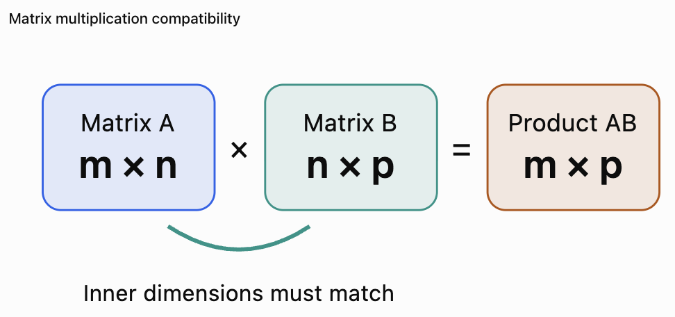
The compatibility rule
Suppose:
A has dimensions m × n.
B has dimensions n × p.
Then the product AB is possible, and the result has dimensions:
m × p
The inner dimensions must match.
|
Matrix A |
Matrix B |
Is AB possible? |
Result |
|---|---|---|---|
|
2 × 3 |
3 × 4 |
Yes |
2 × 4 |
|
3 × 2 |
2 × 5 |
Yes |
3 × 5 |
|
2 × 2 |
2 × 2 |
Yes |
2 × 2 |
|
3 × 4 |
3 × 2 |
No |
Undefined |
|
1 × 3 |
3 × 1 |
Yes |
1 × 1 |
|
3 × 1 |
1 × 3 |
Yes |
3 × 3 |
The outer dimensions determine the size of the result.
How Matrix Multiplication Works
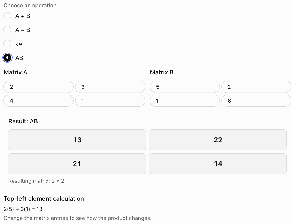
Consider:
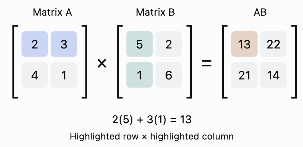
To calculate AB, multiply each row of A by each column of B and add the products.
Finding the first element
Use row 1 of A:
[2, 3]
and column 1 of B:
[5, 1]
Calculate:
2(5) + 3(1) = 13
This becomes the element in row 1, column 1 of AB.
Visualising row-by-column multiplication
Calculating the complete product
Top-left:
2(5) + 3(1) = 13
Top-right:
2(2) + 3(6) = 22
Bottom-left:
4(5) + 1(1) = 21
Bottom-right:
4(2) + 1(6) = 14
Therefore:
General formula
For compatible matrices A and B:
cᵢⱼ = Σ aᵢₖbₖⱼ
The sum is taken over all matching positions k in the row of A and column of B.
In words:
Multiply corresponding entries from the row and column, then add the products.
Worked Example 5: Multiplying a 2 × 3 Matrix by a 3 × 2 Matrix
Given:
Calculate AB.
Step 1: Check compatibility.
A is 2 × 3.
B is 3 × 2.
The inner dimensions are both 3.
Multiplication is possible.
The result will be 2 × 2.
Step 2: Calculate each element.
Row 1 × Column 1:
1(7) + 2(9) + 3(11)
= 7 + 18 + 33
= 58
Row 1 × Column 2:
1(8) + 2(10) + 3(12)
= 8 + 20 + 36
= 64
Row 2 × Column 1:
4(7) + 5(9) + 6(11)
= 28 + 45 + 66
= 139
Row 2 × Column 2:
4(8) + 5(10) + 6(12)
= 32 + 50 + 72
= 154
Step 3: Write the result.
Worked Example 6: Multiplying a Matrix by a Column Vector
Given:
and:
Calculate Ax.
Step 1: Check dimensions.
A is 2 × 2.
x is 2 × 1.
Multiplication is possible.
The result will be 2 × 1.
Step 2: Multiply rows by the column.
First element:
2(5) + 3(2) = 16
Second element:
1(5) + 4(2) = 13
Therefore:
This type of multiplication is especially important in linear algebra, coordinate transformations, and systems of equations.
Why Matrix Multiplication Is Not Usually Commutative
Ordinary multiplication is commutative:
3 × 5 = 5 × 3
However, matrix multiplication generally is not.
AB ≠ BA
Consider:
Calculate AB:
Now calculate BA:
Therefore:
AB ≠ BA
The order matters because multiplying rows by columns produces different combinations of elements.
Sometimes AB is defined while BA is not.
For example:
A: 2 × 3
B: 3 × 4
AB is possible and has dimensions 2 × 4.
BA is not possible because its inner dimensions would be 4 and 2.
Properties of Matrix Multiplication
For compatible matrices:
Associative property
(AB)C = A(BC)
The grouping of multiplication can change without changing the result.
Distributive property
A(B + C) = AB + AC
and:
(A + B)C = AC + BC
provided the operations are defined.
Identity property
AI = A
and:
IA = A
using identity matrices of suitable dimensions.
Scalar compatibility
k(AB) = (kA)B = A(kB)
Noncommutative property
In general:
AB ≠ BA
Zero product property
Unlike ordinary real numbers, it is possible for two nonzero matrices to have a zero product.
For example:
Both matrices are nonzero, but:
AB = O
This is an important difference between ordinary arithmetic and matrix algebra.
Determining Whether Operations Are Possible
Before performing any matrix operation, always check the dimensions.
Addition and subtraction
The matrices must have identical dimensions.
For example:
2 × 3 + 2 × 3 is possible.
2 × 3 + 3 × 2 is not possible.
Scalar multiplication
A scalar can multiply a matrix of any dimensions.
For example:
5A is possible for any matrix A.
Matrix multiplication
The number of columns in the first matrix must equal the number of rows in the second matrix.
For example:
(2 × 4)(4 × 3) is possible.
The result is 2 × 3.
However:
(2 × 4)(2 × 3) is not possible.
Quick compatibility guide
|
Operation |
Requirement |
Result |
|---|---|---|
|
A + B |
Same dimensions |
Same dimensions |
|
A − B |
Same dimensions |
Same dimensions |
|
kA |
Any matrix A |
Same dimensions as A |
|
AB |
Columns of A = rows of B |
Rows of A × columns of B |
|
BA |
Columns of B = rows of A |
Rows of B × columns of A |
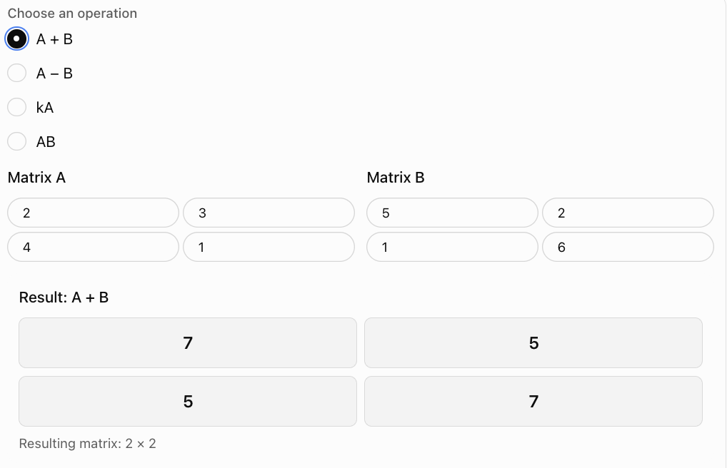
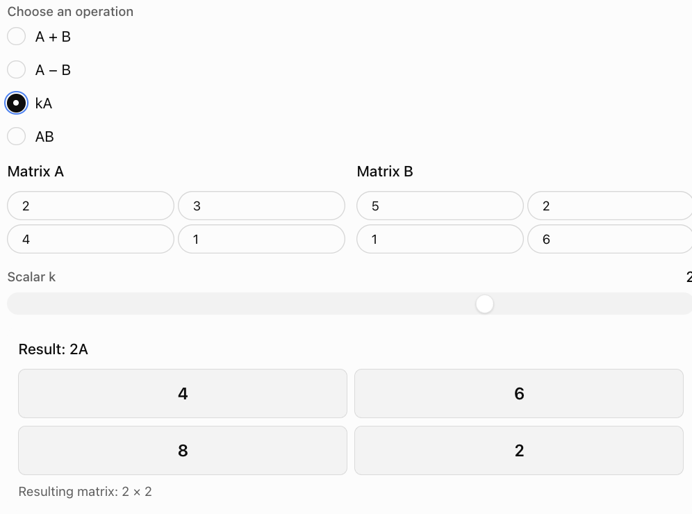
Interactive Matrix Operations Explorer
Explore how addition, subtraction, scalar multiplication, and matrix multiplication work.
Matrix Operations in Real-World Problems
Application 1: Combining Sales Data
Two shops sell three products.
Their weekly sales are represented by:
and:
Rows represent shops.
Columns represent products.
The total sales are:
This provides a compact summary of sales across both weeks.
Application 2: Increasing Production
A factory produces:
If production doubles, the new production matrix is:
Scalar multiplication allows every quantity to be adjusted simultaneously.
Application 3: Calculating Revenue
A shop sells three products.
Quantities sold in two stores are:
The prices of the three products are:
The revenue for each store is calculated using:
R = Qp
Therefore:
-
Store 1 earns $170.
-
Store 2 earns $176.
Matrix multiplication allows the quantities and prices to be combined efficiently.
Matrices and Geometric Transformations
Matrices can describe transformations of points in a coordinate plane.
A point can be represented by a column vector:
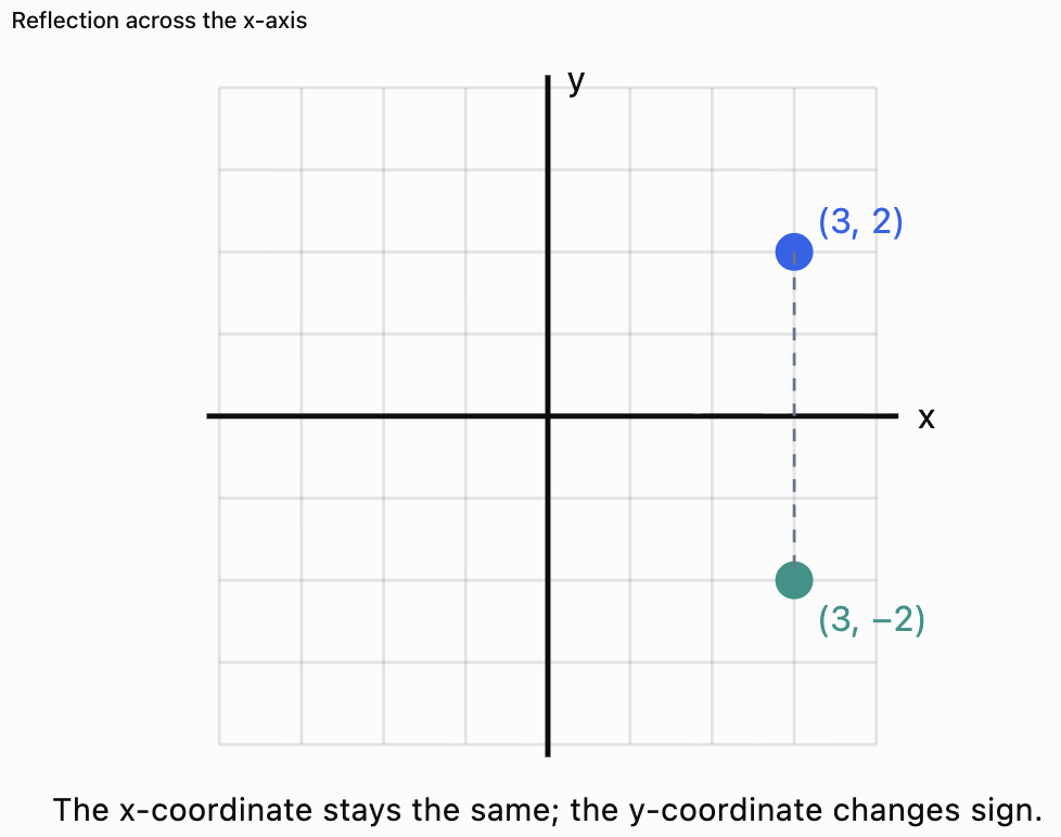
Reflection in the x-axis
The transformation matrix is:
For the point (3, 2):
Calculate:
The point (3, 2) is reflected to (3, −2).
Other transformation matrices can represent:
-
Rotations
-
Reflections
-
Stretches
-
Compressions
-
Shears
These transformations are widely used in computer graphics, animation, robotics, and engineering.
Solving Matrix Equations
Matrix operations can also be used to solve equations involving unknown matrices.
Worked Example 7: Finding an Unknown Matrix
Suppose:
X + A = B
where:
Find X.
Subtract A from both sides:
X = B − A
Therefore:
Worked Example 8: Solving a Matrix Equation with Scalars
Suppose:
2X + A = B
where:
Subtract A:
2X = B − A
Divide every element by 2:
This is equivalent to multiplying the matrix by the scalar 1/2.
Common Mistakes
Mistake 1: Adding matrices with different dimensions
Matrices must have identical dimensions for addition or subtraction.
Mistake 2: Confusing rows and columns
A 2 × 3 matrix has two rows and three columns.
Mistake 3: Forgetting to multiply every element by a scalar
Scalar multiplication affects every element.
Mistake 4: Multiplying corresponding elements during matrix multiplication
Matrix multiplication uses row-by-column products and sums.
Mistake 5: Ignoring the inner dimensions
AB is possible only when the columns of A equal the rows of B.
Mistake 6: Assuming AB = BA
Matrix multiplication is generally not commutative.
Mistake 7: Predicting the wrong result dimensions
The result of an m × n matrix multiplied by an n × p matrix is m × p.
Mistake 8: Making sign errors
Negative elements require careful handling.
Mistake 9: Reversing the order of multiplication
AB and BA may produce different results or one may be undefined.
Mistake 10: Forgetting to interpret the result
In applications, matrix elements represent real quantities such as prices, distances, or measurements.
Key Terms
-
Matrix: Rectangular arrangement of elements in rows and columns.
-
Element: Individual entry in a matrix.
-
Row: Horizontal arrangement of elements.
-
Column: Vertical arrangement of elements.
-
Order: Dimensions of a matrix, written as rows × columns.
-
Row Matrix: Matrix containing one row.
-
Column Matrix: Matrix containing one column.
-
Square Matrix: Matrix with equal numbers of rows and columns.
-
Zero Matrix: Matrix in which every element is zero.
-
Identity Matrix: Square matrix with 1 on the main diagonal and 0 elsewhere.
-
Scalar: Single number used to multiply a matrix.
-
Matrix Addition: Operation combining corresponding elements of matrices with identical dimensions.
-
Matrix Subtraction: Operation subtracting corresponding elements.
-
Scalar Multiplication: Multiplication of every matrix element by a scalar.
-
Matrix Multiplication: Operation combining rows and columns through products and sums.
-
Compatible Matrices: Matrices whose dimensions allow a particular operation.
-
Matrix Product: Result of multiplying compatible matrices.
-
Commutative Property: Property stating that changing the order of an operation does not change the result.
-
Associative Property: Property allowing the grouping of operations to change.
-
Distributive Property: Property relating multiplication to addition.
-
Additive Inverse: Matrix that produces the zero matrix when added to the original.
-
Transformation Matrix: Matrix representing a geometric transformation.
-
Column Vector: Matrix consisting of one column.
-
Matrix Equation: Equation containing one or more matrices.
-
Linear Algebra: Branch of mathematics involving vectors, matrices, and linear relationships.
Key Takeaways
-
Matrices organise information into rows and columns.
-
Matrix dimensions are written as rows × columns.
-
Matrices can be added or subtracted only when they have identical dimensions.
-
Addition and subtraction are performed element by element.
-
Scalar multiplication multiplies every element by the same number.
-
Matrix multiplication requires compatible inner dimensions.
-
The result of multiplying an m × n matrix by an n × p matrix has dimensions m × p.
-
Matrix multiplication uses row-by-column calculations.
-
Matrix multiplication is generally not commutative.
-
Addition and scalar multiplication follow useful algebraic properties.
-
Identity matrices play a role similar to the number 1 in multiplication.
-
Matrices can represent data, transformations, and systems of equations.
-
Matrix operations are useful in finance, science, engineering, and computer graphics.
-
Checking dimensions before calculating helps prevent errors.
Check Your Understanding
Questions
Question 1: Matrix Dimensions
Determine the dimensions of:
Question 2: Matrix Addition
Calculate:
Question 3: Matrix Subtraction
Calculate:
Question 4: Scalar Multiplication
Calculate:
Question 5: Negative Scalar
Calculate:
Question 6: Compatibility
Determine whether the product AB is possible if:
A is 3 × 4.
B is 4 × 2.
State the dimensions of the result.
Question 7: Incompatible Matrices
Explain why a 2 × 3 matrix cannot be multiplied on the right by a 4 × 2 matrix.
Question 8: Matrix Multiplication
Calculate:
Question 9: Matrix and Column Vector
Calculate:
Question 10: Combined Operations
Given:
Calculate 2A + B.
Question 11: Matrix Equations
Solve:
X + A = B
where:
Question 12: Noncommutative Multiplication
Explain why AB is not always equal to BA.
Question 13: Revenue Calculation
A shop sells two products.
The quantities sold are:
The prices are:
Calculate Qp and interpret the result.
Question 14: Geometric Transformation
Use the matrix:
to transform the point (4, 3).
Question 15: Integrated Matrix Challenge
Given:
Calculate:
a) A + B
b) A − B
c) 3A
d) AB
e) BA
f) Explain whether AB = BA.
Fully Worked Answers
Answer 1: Matrix Dimensions
The matrix has two rows and three columns.
Answer: 2 × 3
Answer 2: Matrix Addition
Answer 3: Matrix Subtraction
Answer 4: Scalar Multiplication
Answer 5: Negative Scalar
Answer 6: Compatibility
A is 3 × 4.
B is 4 × 2.
The inner dimensions are both 4.
Multiplication is possible.
Result: 3 × 2
Answer 7: Incompatible Matrices
A is 2 × 3.
B is 4 × 2.
The inner dimensions are 3 and 4.
They do not match.
Therefore, AB is undefined.
Answer 8: Matrix Multiplication
Top-left:
1(5) + 2(7) = 19
Top-right:
1(6) + 2(8) = 22
Bottom-left:
3(5) + 4(7) = 43
Bottom-right:
3(6) + 4(8) = 50
Answer 9: Matrix and Column Vector
First element:
2(5) + 1(2) = 12
Second element:
4(5) + 3(2) = 26
Answer 10: Combined Operations
First:
Add B:
Answer 11: Matrix Equations
Given:
X + A = B
Subtract A:
X = B − A
Answer 12: Noncommutative Multiplication
Matrix multiplication uses rows from the first matrix and columns from the second matrix.
Reversing the order changes which rows and columns are combined.
Therefore, AB and BA generally produce different results.
Sometimes one product is possible while the other is undefined.
Answer 13: Revenue Calculation
First store:
10(4) + 20(6)
= 40 + 120
= 160
Second store:
15(4) + 12(6)
= 60 + 72
= 132
The first store earns $160.
The second store earns $132.
Answer 14: Geometric Transformation
Given:
and:
Calculate:
Answer: (−4, 3)
The transformation is a reflection in the y-axis.
Answer 15: Integrated Matrix Challenge
Given:
Part a: A + B
Part b: A − B
Part c: 3A
Part d: AB
Top-left:
2(1) + 1(2) = 4
Top-right:
2(5) + 1(3) = 13
Bottom-left:
3(1) + 4(2) = 11
Bottom-right:
3(5) + 4(3) = 27
Part e: BA
Top-left:
1(2) + 5(3) = 17
Top-right:
1(1) + 5(4) = 21
Bottom-left:
2(2) + 3(3) = 13
Bottom-right:
2(1) + 3(4) = 14
Part f: Compare AB and BA
The matrices are different.
Therefore:
AB ≠ BA
This demonstrates that matrix multiplication is not generally commutative.
Final Reflection
Matrix operations extend familiar arithmetic ideas into a powerful system for working with organised numerical information.
Addition and subtraction allow us to combine or compare datasets. Scalar multiplication changes every element by the same factor. Matrix multiplication creates new relationships by combining rows and columns.
These operations are not arbitrary rules. They provide the mathematical foundation for many important applications, including computer graphics, engineering, scientific modeling, economics, and systems of equations.
One of the most important skills is recognising when an operation is possible. Checking matrix dimensions before calculating prevents many common errors.
The central idea is that matrices allow us to organise and manipulate multiple related quantities efficiently, while the rules of matrix operations ensure that the calculations remain mathematically meaningful.
3. Determinants
Learning outcomes
- I can calculate determinants of 2×2 and 3×3 matrices.
- I can interpret the meaning of determinants.
- I can determine whether matrices are invertible.
- I can apply determinants to geometric problems.
- I can solve determinant-based problems.
Introduction
Matrices allow us to organise numbers, represent transformations, and solve systems of equations. However, matrices also have important properties that cannot be determined simply by looking at their individual elements.
One of these properties is the determinant.
A determinant is a single number calculated from a square matrix. Although it produces only one value, that value reveals important information about the matrix.
For example, the determinant can tell us whether:
-
A matrix has an inverse.
-
A system of linear equations has a unique solution.
-
A geometric transformation enlarges or reduces an area or volume.
-
A transformation reverses orientation.
-
Points in a coordinate plane lie on the same straight line.
Consider the matrix:
Its determinant is:
det(A) = 3(4) − 2(1) = 10
This value has several interpretations. Geometrically, the transformation represented by A multiplies areas by 10. Algebraically, because the determinant is not zero, the matrix has an inverse.
Determinants therefore connect matrix algebra with geometry, transformations, and systems of equations.
What Is a Determinant?
The determinant is a scalar value associated with a square matrix.
A square matrix has the same number of rows and columns.
For example:
The determinant can be written as:
det(A)
or:
Although vertical bars are also used for absolute value, the determinant is a different operation.
A determinant can be positive, negative, or zero.
Important properties
-
Determinants are defined for square matrices.
-
The determinant of a 2 × 2 matrix is calculated using four elements.
-
The determinant of a 3 × 3 matrix is calculated using nine elements.
-
A nonzero determinant indicates that a square matrix is invertible.
-
A zero determinant indicates that a square matrix is singular.
-
The absolute value of a determinant describes an area or volume scaling factor.
The sign of the determinant provides information about orientation.
Calculating the Determinant of a 2 × 2 Matrix
For a matrix:
the determinant is:
This is one of the most important formulas in introductory matrix algebra.
Visualising the formula
The determinant of a 2 × 2 matrix
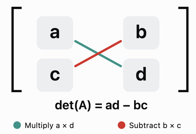
The process is:
-
Multiply the top-left element by the bottom-right element.
-
Multiply the top-right element by the bottom-left element.
-
Subtract the second product from the first.
Worked Example 1: Positive Determinant
Calculate:
Using:
det(A) = ad − bc
Substitute:
det(A) = 4(5) − 2(3)
= 20 − 6
det(A) = 14
The determinant is positive and nonzero.
Therefore, the matrix is invertible.
Worked Example 2: Negative Determinant
Calculate:
det(B) = 2(3) − 5(4)
= 6 − 20
det(B) = −14
The determinant is negative.
This indicates that the associated linear transformation reverses orientation.
The area scaling factor is |−14| = 14.
Worked Example 3: Zero Determinant
Calculate:
det(C) = 2(6) − 4(3)
= 12 − 12
det(C) = 0
The second column is twice the first column.
The columns are linearly dependent.
This matrix is singular and does not have an inverse.
Calculating the Determinant of a 3 × 3 Matrix
Consider the general matrix:
The determinant is:
This formula can be understood through cofactor expansion.
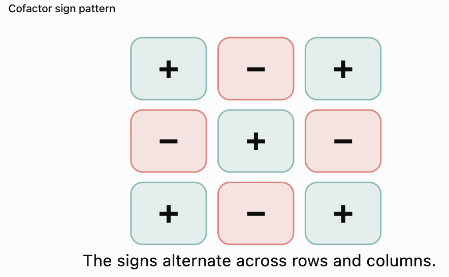
Cofactor expansion along the first row
Each element in the first row is multiplied by the determinant of a smaller 2 × 2 matrix.
The signs follow the pattern:
+ − +
What is a minor?
The minor of an element is the determinant of the smaller matrix formed by removing the row and column containing that element.
For example, for the top-left element a:
Remove the first row and first column.
The remaining matrix is:
Its determinant is:
ei − fh
This is the minor associated with a.
A cofactor is the minor multiplied by the appropriate positive or negative sign.
Worked Example 4: Determinant of a 3 × 3 Matrix
Calculate:
Expand along the first row.
Step 1: Apply the cofactor expansion formula.
det(A) = 2(4 × 6 − 5 × 2) − 1(0 × 6 − 5 × 1) + 3(0 × 2 − 4 × 1)
Step 2: Calculate the 2 × 2 determinants.
First:
4(6) − 5(2) = 24 − 10 = 14
Second:
0(6) − 5(1) = −5
Third:
0(2) − 4(1) = −4
Step 3: Substitute.
det(A) = 2(14) − 1(−5) + 3(−4)
= 28 + 5 − 12
det(A) = 21
The matrix is invertible because its determinant is nonzero.
Worked Example 5: Expanding Along a Row Containing Zeros
Consider:
Expanding along the first row is particularly efficient because two elements are zero.
det(B) = 3(4 × 6 − 1 × 2)
= 3(24 − 2)
= 3(22)
det(B) = 66
This example demonstrates an important strategy:
When calculating a 3 × 3 determinant, choose a row or column containing the most zeros whenever possible.
The Rule of Sarrus
Another method for calculating a 3 × 3 determinant is the Rule of Sarrus.
This method uses diagonal products.
For:
the determinant is:
det(A) = aei + bfg + cdh − ceg − bdi − afh
Visualising Sarrus' Rule
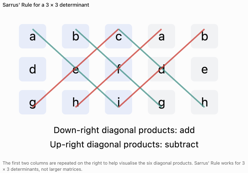
Worked Example 6: Using Sarrus' Rule
Calculate:
Add the downward diagonal products:
1(5)(10) + 2(6)(7) + 3(4)(8)
= 50 + 84 + 96
= 230
Add the upward diagonal products:
3(5)(7) + 2(4)(10) + 1(6)(8)
= 105 + 80 + 48
= 233
Subtract:
det(C) = 230 − 233
det(C) = −3
Properties of Determinants
Determinants follow several important algebraic rules.
Property 1: Identity matrix
The determinant of an identity matrix is 1.
det(I) = 1
For example:
Property 2: Interchanging two rows
Swapping two rows changes the sign of the determinant.
If det(A) = 5, then swapping two rows produces a matrix with determinant −5.
Property 3: Identical rows
If two rows are identical, the determinant is zero.
For example:
Property 4: Proportional rows
If one row is a multiple of another, the determinant is zero.
Property 5: Multiplying one row by a scalar
Multiplying one row by k multiplies the determinant by k.
Property 6: Adding a multiple of one row to another
Adding a multiple of one row to another row does not change the determinant.
This property is especially useful when simplifying larger determinants.
Property 7: Triangular matrices
The determinant of an upper or lower triangular matrix equals the product of its diagonal elements.
For example:
det(A) = 2 × 5 × 7
det(A) = 70
Property 8: Product of matrices
For square matrices of the same order:
det(AB) = det(A)det(B)
Property 9: Transpose
The determinant does not change when rows and columns are interchanged.
det(Aᵀ) = det(A)
Property 10: Scalar multiplication
For an n × n matrix:
det(kA) = kⁿdet(A)
For example, for a 2 × 2 matrix:
det(3A) = 3²det(A) = 9det(A)
This is different from simply multiplying the determinant by 3.
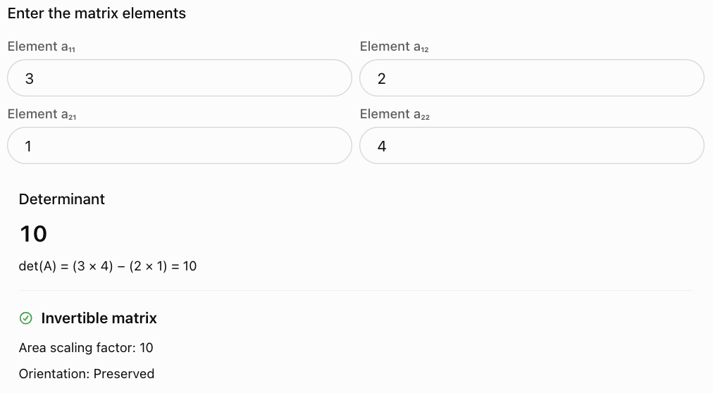
Try changing the values so that the determinant becomes zero. What relationships do you notice between the rows or columns?
Determinants and Invertible Matrices
A square matrix is invertible if another matrix exists that reverses its effect under multiplication.
For an invertible matrix A:
AA⁻¹ = A⁻¹A = I
where:
-
A⁻¹ is the inverse matrix.
-
I is the identity matrix.
The determinant tells us whether an inverse exists.
Invertibility condition
If det(A) ≠ 0, the matrix is invertible.
If det(A) = 0, the matrix is singular and not invertible.
This is one of the most important applications of determinants.
Formula for the inverse of a 2 × 2 matrix
For:
if ad − bc ≠ 0:
Worked Example 7: Finding an Inverse
Given:
Step 1: Calculate the determinant.
det(A) = 4(3) − 1(2)
= 12 − 2
= 10
Since det(A) ≠ 0, an inverse exists.
Step 2: Apply the inverse formula.
Therefore:
Worked Example 8: Identifying a Singular Matrix
Given:
det(B) = 6(3) − 9(2)
= 18 − 18
= 0
Therefore, B is singular.
B has no inverse.
The first row is three times the second row, so the rows are linearly dependent.
Geometric Meaning of Determinants
Determinants have a powerful geometric interpretation.
For a 2 × 2 matrix, the absolute value of the determinant represents the factor by which a linear transformation changes area.
For a 3 × 3 matrix, the absolute value of the determinant represents the factor by which a linear transformation changes volume.
Area scaling in two dimensions
Suppose:
This transformation:
-
Multiplies x-coordinates by 2.
-
Multiplies y-coordinates by 3.
The determinant is:
det(A) = 2(3) − 0(0)
det(A) = 6
Therefore, areas are multiplied by 6.
A square with area 1 becomes a rectangle with area 6.
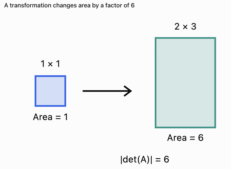
Positive and negative determinants
A positive determinant means the transformation preserves orientation.
A negative determinant means the transformation reverses orientation.
For example, a reflection in the x-axis has matrix:
Its determinant is:
det(R) = 1(−1) − 0(0)
det(R) = −1
The area is unchanged because |−1| = 1.
However, orientation is reversed.
Zero determinant
If det(A) = 0, a transformation collapses space into a lower-dimensional set.
For example:
det(A) = 4 − 4 = 0
The transformation maps the entire plane onto a line.
Areas become zero.
This explains geometrically why the matrix cannot be inverted: different points can be mapped to the same location.
Determinants and the Area of a Parallelogram
Suppose two vectors are:
u = (a, c)
v = (b, d)
These vectors form adjacent sides of a parallelogram.
Its area is:
This is the absolute value of the determinant:
Worked Example 9: Parallelogram Area
Two vectors are:
u = (3, 1)
v = (2, 4)
Construct the matrix:
Calculate:
det(A) = 3(4) − 2(1)
= 12 − 2
= 10
Therefore:
Area = 10 square units
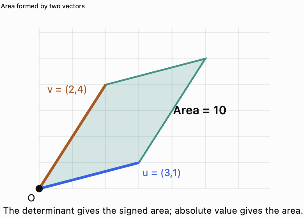
Determinants and the Area of a Triangle
A triangle formed by two vectors has half the area of the parallelogram formed by those vectors.
Therefore:
Worked Example 10: Triangle Area from Coordinates
Find the area of the triangle with vertices:
A(1, 2)
B(5, 3)
C(3, 7)
Step 1: Form two vectors from A.
AB = (5 − 1, 3 − 2)
AB = (4, 1)
AC = (3 − 1, 7 − 2)
AC = (2, 5)
Step 2: Construct the matrix.
Step 3: Calculate the determinant.
det(M) = 4(5) − 2(1)
= 20 − 2
= 18
Step 4: Divide by 2.
Area = 1/2 × |18|
Area = 9 square units
Coordinate formula
For vertices (x₁, y₁), (x₂, y₂), and (x₃, y₃):
Area = 1/2 |x₁(y₂ − y₃) + x₂(y₃ − y₁) + x₃(y₁ − y₂)|
This formula can also be written as a 3 × 3 determinant:
Determinants and Collinear Points
Three points are collinear if they lie on the same straight line.
A determinant can be used to test collinearity.
For points A(x₁, y₁), B(x₂, y₂), and C(x₃, y₃), calculate:
If D = 0, the three points are collinear.
Worked Example 11: Testing Collinearity
Determine whether the points:
A(1, 2)
B(3, 6)
C(5, 10)
are collinear.
Construct:
Expand along the first row:
D = 1(6 − 10) − 2(3 − 5) + 1(30 − 30)
= −4 − 2(−2) + 0
= −4 + 4
D = 0
Therefore, the points are collinear.
This agrees with the fact that all three points satisfy:
y = 2x
Determinants and Volume in Three Dimensions
A 3 × 3 determinant represents the signed volume scaling factor of a linear transformation in three-dimensional space.
If three vectors form the edges of a parallelepiped, its volume is the absolute value of their determinant.
Worked Example 12: Volume of a Parallelepiped
Consider three vectors:
u = (2, 0, 0)
v = (0, 3, 0)
w = (0, 0, 4)
Construct:
Since this is a diagonal matrix:
det(A) = 2 × 3 × 4
= 24
Therefore:
Volume = 24 cubic units
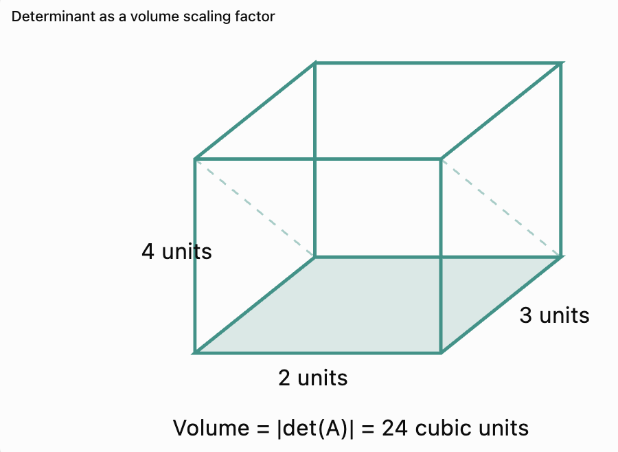
For a general parallelepiped, the vectors do not need to be perpendicular. The determinant still gives its signed volume.
Determinants and Systems of Linear Equations
Determinants can be used to determine whether a system of linear equations has a unique solution.
Consider:
ax + by = e
cx + dy = f
The coefficient matrix is:
If det(A) ≠ 0, the system has exactly one solution.
If det(A) = 0, the system does not have a unique solution. It may have no solutions or infinitely many solutions.
Cramer's Rule
For a system:
ax + by = e
cx + dy = f
Define:
D = ad − bc
Dₓ = ed − bf
Dᵧ = af − ec
If D ≠ 0:
Worked Example 13: Solving a System Using Determinants
Solve:
2x + 3y = 12
4x − y = 5
Step 1: Calculate D.
D = 2(−1) − 3(4)
= −2 − 12
= −14
Step 2: Calculate Dₓ.
Replace the x-coefficient column with the constants.
Dₓ = 12(−1) − 3(5)
= −12 − 15
= −27
Step 3: Calculate Dᵧ.
Replace the y-coefficient column with the constants.
Dᵧ = 2(5) − 12(4)
= 10 − 48
= −38
Step 4: Solve.
x = Dₓ/D = −27/−14
x = 27/14
y = Dᵧ/D = −38/−14
y = 19/7
Step 5: Verify.
First equation:
2(27/14) + 3(19/7)
= 27/7 + 57/7
= 84/7
= 12
Second equation:
4(27/14) − 19/7
= 54/7 − 19/7
= 35/7
= 5
Both equations are satisfied.
Solving Determinant Equations
Sometimes the determinant is known, but one matrix element is unknown.
Worked Example 14: Finding an Unknown Element
Suppose:
Find x.
Using the 2 × 2 determinant formula:
5x − 3(2) = 14
5x − 6 = 14
5x = 20
x = 4
Worked Example 15: Finding When a Matrix Is Singular
Determine the values of k for which:
is singular.
A matrix is singular when its determinant is zero.
Therefore:
det(A) = 0
k² − 2(8) = 0
k² − 16 = 0
Factor:
(k − 4)(k + 4) = 0
Therefore:
k = 4 or k = −4
For either value, the matrix has no inverse.
Real-World Applications of Determinants
Computer graphics
Determinants help determine how transformations scale areas and volumes, and whether they reverse orientation.
Robotics
Determinants help identify singular configurations in mathematical models of robot movement, where certain motions become difficult or impossible to control independently.
Engineering
Determinants help analyse linear systems describing forces, constraints, and structural relationships.
Surveying and geometry
Determinants allow areas of triangles and parallelograms to be calculated directly from coordinates.
Scientific modelling
Determinants help identify whether linear systems have unique solutions and whether transformations preserve independent directions.
Common Mistakes
Mistake 1: Calculating determinants for non-square matrices
Determinants are defined only for square matrices.
Mistake 2: Reversing the subtraction in a 2 × 2 determinant
The correct formula is:
ad − bc
not bc − ad.
Mistake 3: Forgetting the alternating signs in 3 × 3 expansion
The first-row cofactor signs are:
+ − +
Mistake 4: Confusing determinants with absolute values
A determinant may be negative.
Absolute value is used when calculating geometric area or volume.
Mistake 5: Assuming a zero determinant means every matrix element is zero
A matrix can contain many nonzero elements and still have determinant zero.
Mistake 6: Assuming every square matrix has an inverse
Only square matrices with nonzero determinants are invertible.
Mistake 7: Applying Sarrus' Rule to larger matrices
Sarrus' Rule applies specifically to 3 × 3 determinants.
Mistake 8: Multiplying every element by a scalar without accounting for matrix order
For an n × n matrix:
det(kA) = kⁿdet(A)
Mistake 9: Ignoring negative signs in cofactor expansion
Subtracting a negative minor produces a positive contribution.
Mistake 10: Confusing determinant and area
The determinant gives signed area scaling. Geometric area is always nonnegative.
Mistake 11: Using Cramer's Rule when the determinant is zero
Cramer's Rule requires a nonzero coefficient determinant.
Mistake 12: Assuming det(A) = 0 always means no solution
A linear system with determinant zero may have no solutions or infinitely many solutions.
Key Terms
-
Determinant: Scalar value calculated from a square matrix.
-
Square Matrix: Matrix with equal numbers of rows and columns.
-
Scalar: Single numerical value.
-
Minor: Determinant obtained by deleting a specified row and column.
-
Cofactor: Signed minor associated with a matrix element.
-
Cofactor Expansion: Method for calculating determinants using minors and cofactors.
-
Rule of Sarrus: Diagonal method for calculating 3 × 3 determinants.
-
Invertible Matrix: Square matrix with a multiplicative inverse.
-
Inverse Matrix: Matrix that produces the identity matrix when multiplied by the original matrix.
-
Singular Matrix: Square matrix with determinant zero.
-
Nonsingular Matrix: Square matrix with a nonzero determinant.
-
Identity Matrix: Square matrix with 1 on the main diagonal and 0 elsewhere.
-
Main Diagonal: Diagonal extending from the top-left to the bottom-right of a matrix.
-
Triangular Matrix: Square matrix with zeros above or below the main diagonal.
-
Linear Transformation: Mapping represented by multiplication by a matrix.
-
Orientation: Directional arrangement preserved or reversed by a transformation.
-
Area Scaling Factor: Absolute value of a 2 × 2 transformation determinant.
-
Volume Scaling Factor: Absolute value of a 3 × 3 transformation determinant.
-
Parallelogram: Quadrilateral with opposite sides parallel.
-
Parallelepiped: Three-dimensional solid with parallelogram faces.
-
Collinear Points: Points lying on the same straight line.
-
Linear Dependence: Relationship in which one vector can be expressed using others.
-
Cramer's Rule: Method for solving certain linear systems using determinants.
-
Coefficient Matrix: Matrix containing the coefficients of a linear system.
-
Unique Solution: Exactly one solution satisfying a system of equations.
-
Row Operation: Operation performed on rows of a matrix.
-
Transpose: Matrix obtained by interchanging rows and columns.
Key Takeaways
-
Determinants are scalar values associated with square matrices.
-
The determinant of a 2 × 2 matrix is ad − bc.
-
A 3 × 3 determinant can be calculated using cofactor expansion or Sarrus' Rule.
-
Cofactor expansion uses alternating positive and negative signs.
-
A determinant can be positive, negative, or zero.
-
A square matrix is invertible exactly when its determinant is nonzero.
-
A zero determinant indicates a singular matrix.
-
The determinant of a triangular matrix is the product of its diagonal elements.
-
Swapping two rows reverses the determinant's sign.
-
Proportional rows or columns produce a zero determinant.
-
For square matrices, det(AB) = det(A)det(B).
-
The absolute value of a 2 × 2 determinant gives an area scaling factor.
-
The absolute value of a 3 × 3 determinant gives a volume scaling factor.
-
Determinants can calculate areas of triangles and parallelograms.
-
Determinants can test whether three points are collinear.
-
Cramer's Rule uses determinants to solve systems with unique solutions.
-
Determinants connect algebra, geometry, transformations, and scientific applications.
Check Your Understanding
Questions
Question 1: Basic Determinant
Calculate:
Question 2: Negative Determinant
Calculate:
Question 3: Zero Determinant
Determine whether:
is invertible.
Question 4: 3 × 3 Determinant
Calculate:
Question 5: Triangular Matrix
Find the determinant of:
Question 6: Determinant Properties
If det(A) = 7, what happens to the determinant when two rows are swapped?
Question 7: Scalar Multiplication
If A is a 2 × 2 matrix and det(A) = 5, calculate det(3A).
Question 8: Invertibility
Determine whether:
has an inverse.
Question 9: Finding an Unknown
Solve:
Question 10: Singular Matrix
Find k if:
is singular.
Question 11: Parallelogram Area
Find the area of the parallelogram formed by:
u = (4, 1)
v = (2, 5)
Question 12: Triangle Area
Find the area of the triangle with vertices:
A(0, 0), B(6, 0), C(2, 4).
Question 13: Volume
Calculate the volume of the parallelepiped formed by the column vectors of:
Question 14: Cramer's Rule
Solve using determinants:
3x + 2y = 12
x − y = 1
Question 15: Integrated Determinant Challenge
Given:
a) Calculate det(A).
b) Determine whether A is invertible.
c) Explain the geometric meaning of the determinant.
d) Calculate det(2A).
Fully Worked Answers
Answer 1: Basic Determinant
det(A) = 3(5) − 2(4)
= 15 − 8
Answer: 7
Answer 2: Negative Determinant
det(A) = 1(2) − 6(3)
= 2 − 18
Answer: −16
Answer 3: Zero Determinant
det(A) = 2(10) − 4(5)
= 20 − 20
= 0
The determinant is zero.
Answer: The matrix is singular and not invertible.
Answer 4: 3 × 3 Determinant
Expand along the first row:
det(A) = 1(4 × 6 − 5 × 0) − 2(0 × 6 − 5 × 1) + 3(0 × 0 − 4 × 1)
= 1(24) − 2(−5) + 3(−4)
= 24 + 10 − 12
Answer: 22
Answer 5: Triangular Matrix
The matrix is upper triangular.
Multiply the diagonal elements:
det(A) = 3 × 4 × 6
Answer: 72
Answer 6: Determinant Properties
Swapping two rows changes the sign of the determinant.
Original determinant:
7
New determinant:
Answer: −7
Answer 7: Scalar Multiplication
For a 2 × 2 matrix:
det(kA) = k²det(A)
Therefore:
det(3A) = 3²(5)
= 9(5)
Answer: 45
Answer 8: Invertibility
det(B) = 4(5) − 3(2)
= 20 − 6
= 14
Since det(B) ≠ 0:
Answer: B is invertible.
Answer 9: Finding an Unknown
4x − 6 = 10
4x = 16
Answer: x = 4
Answer 10: Singular Matrix
A singular matrix has determinant zero.
6k − 12 = 0
6k = 12
Answer: k = 2
Answer 11: Parallelogram Area
Vectors:
u = (4, 1)
v = (2, 5)
Area = |4(5) − 2(1)|
= |20 − 2|
Answer: 18 square units
Answer 12: Triangle Area
Vertices:
A(0, 0)
B(6, 0)
C(2, 4)
Vectors:
AB = (6, 0)
AC = (2, 4)
Area = 1/2 |6(4) − 2(0)|
= 1/2 |24|
Answer: 12 square units
Answer 13: Volume
The matrix is diagonal.
det(A) = 2 × 5 × 3
= 30
Volume = |det(A)|
Answer: 30 cubic units
Answer 14: Cramer's Rule
Equations:
3x + 2y = 12
x − y = 1
Step 1: Calculate D.
D = 3(−1) − 2(1)
= −3 − 2
= −5
Step 2: Calculate Dₓ.
Dₓ = 12(−1) − 2(1)
= −14
Step 3: Calculate Dᵧ.
Dᵧ = 3(1) − 12(1)
= −9
Step 4: Solve.
x = Dₓ/D
= −14/−5
x = 14/5
y = Dᵧ/D
= −9/−5
y = 9/5
Verification:
3(14/5) + 2(9/5)
= 42/5 + 18/5
= 60/5 = 12
14/5 − 9/5 = 1
Both equations are satisfied.
Answer 15: Integrated Determinant Challenge
Given:
Part a: Calculate det(A).
Expand along the first row:
det(A) = 2(4 × 5 − 2 × 0) − 1(3 × 5 − 2 × 1) + 0
= 2(20) − (15 − 2)
= 40 − 13
det(A) = 27
Part b: Determine invertibility.
Since det(A) = 27 ≠ 0:
A is invertible.
Part c: Geometric interpretation.
The matrix represents a linear transformation in three-dimensional space.
Its determinant is 27.
Therefore, volumes are multiplied by:
|27| = 27
Because the determinant is positive, orientation is preserved.
Part d: Calculate det(2A).
For a 3 × 3 matrix:
det(kA) = k³det(A)
Therefore:
det(2A) = 2³(27)
= 8(27)
det(2A) = 216
Final Reflection
Determinants are much more than a calculation involving matrix elements.
They reveal fundamental properties of matrices and the transformations they represent.
A nonzero determinant tells us that a matrix is invertible and that the associated linear transformation does not collapse space into a lower dimension. A zero determinant indicates that some information is lost and the transformation cannot be reversed.
Geometrically, determinants connect matrix algebra to area, volume, orientation, and coordinate geometry. Algebraically, they provide tools for solving systems of equations and determining whether unique solutions exist.
By mastering 2 × 2 and 3 × 3 determinants, understanding their properties, and applying them to geometric and algebraic problems, we develop an important foundation for further study of linear algebra.
The central idea is that a determinant is a single number that reveals whether a matrix preserves independent dimensions, how it changes area or volume, and whether its transformation can be reversed.
4. Inverse Matrices
Learning outcomes
- I can calculate inverse matrices.
- I can verify inverse matrices.
- I can solve equations using matrix inverses.
- I can recognise singular matrices.
- I can apply inverse matrices in practical situations.
Introduction
In ordinary arithmetic, many operations can be reversed.
For example, if a number is multiplied by 5, we can reverse the operation by dividing by 5.
5 × 8 = 40
40 ÷ 5 = 8
Matrices have a similar idea. Under certain conditions, a matrix multiplication can be reversed using an inverse matrix.
Suppose a matrix A transforms a vector x into another vector b:
Ax = b
If A has an inverse, we can use that inverse to recover the original vector:
x = A⁻¹b
Inverse matrices are important because they allow us to solve systems of linear equations, reverse geometric transformations, recover original data, and analyse mathematical models.
However, not every matrix has an inverse. Some transformations lose information, making it impossible to recover the original values uniquely.
In this lesson, we will investigate how inverse matrices are calculated, verified, and applied to mathematical and real-world problems.
What Is an Inverse Matrix?
The inverse matrix of a square matrix A is another matrix, written as A⁻¹, that reverses the effect of multiplication by A.
The defining property is:
AA⁻¹ = A⁻¹A = I
where I is the identity matrix.
For a 2 × 2 matrix, the identity matrix is:
The identity matrix plays a role similar to the number 1 in ordinary multiplication.
For example:
5 × 1 = 5
Similarly:
AI = IA = A
Understanding the relationship
If:
Ax = b
then multiplying both sides on the left by A⁻¹ gives:
A⁻¹Ax = A⁻¹b
Since:
A⁻¹A = I
we obtain:
Ix = A⁻¹b
Therefore:
This relationship is fundamental to solving linear systems using matrices.
Visualising inverse transformations
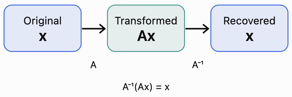
The inverse matrix undoes the original transformation.
Conditions for an Inverse Matrix to Exist
A matrix must satisfy certain conditions before it can have an inverse.
Condition 1: The matrix must be square
A square matrix has the same number of rows and columns.
Examples include:
-
2 × 2 matrices
-
3 × 3 matrices
-
4 × 4 matrices
A rectangular matrix does not have an ordinary two-sided inverse, although some rectangular matrices have specialised one-sided or generalised inverses.
Condition 2: The determinant must not be zero
A square matrix is invertible exactly when:
det(A) ≠ 0
If:
det(A) = 0
the matrix is called singular and does not have an inverse.
Worked Example 1: Checking Invertibility
Consider:
Calculate the determinant:
det(A) = 3(4) − 2(1)
= 12 − 2
= 10
Since det(A) ≠ 0:
A is invertible.
Now consider:
det(B) = 2(6) − 4(3)
= 12 − 12
= 0
Therefore:
B is singular and has no inverse.
Calculating the Inverse of a 2 × 2 Matrix
For a matrix:
the inverse is:
provided:
ad − bc ≠ 0
The four-step method
-
Calculate the determinant: ad − bc.
-
Check that the determinant is not zero.
-
Exchange the positions of a and d, and change the signs of b and c.
-
Multiply every element by 1/det(A).
Visualising the inverse formula
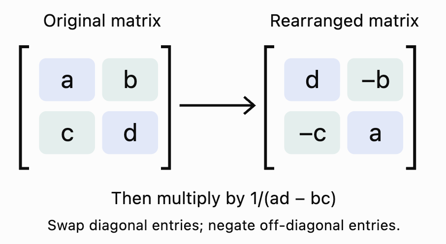
Worked Example 2: Finding an Inverse Matrix
Calculate the inverse of:
Step 1: Calculate the determinant.
det(A) = 4(3) − 1(2)
= 12 − 2
= 10
Step 2: Check invertibility.
Since det(A) = 10 ≠ 0, the inverse exists.
Step 3: Exchange the diagonal elements and change the signs of the other elements.
Step 4: Multiply by 1/10.
Therefore:
Fractions may be preferable when exact answers are required.
Worked Example 3: Inverse with a Negative Determinant
Find the inverse of:
Step 1: Calculate the determinant.
det(B) = 2(4) − 5(3)
= 8 − 15
= −7
Step 2: Apply the inverse formula.
Therefore:
A negative determinant does not prevent a matrix from having an inverse.
Only a zero determinant prevents invertibility.
Verifying Inverse Matrices
Calculating an inverse is only part of the process.
We should also be able to verify that the inverse is correct.
Two square matrices A and B are inverses if:
AB = BA = I
For square matrices of the same order, verifying either AB = I or BA = I is mathematically sufficient, but checking both is useful practice.
Worked Example 4: Verifying an Inverse
Given:
and:
Determine whether B is the inverse of A.
Step 1: Calculate AB.
Top-left:
2(2) + 1(−3) = 1
Top-right:
2(−1) + 1(2) = 0
Bottom-left:
3(2) + 2(−3) = 0
Bottom-right:
3(−1) + 2(2) = 1
Therefore:
Step 2: Calculate BA.
Therefore:
B = A⁻¹
The inverse has been verified.
Interactive Inverse Matrix Explorer
Change the elements of a 2 × 2 matrix to investigate its determinant, inverse, and invertibility.
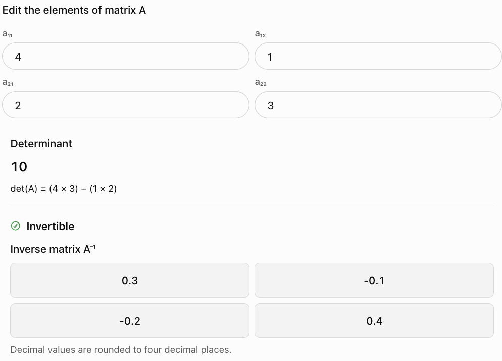
Finding Inverses Using Row Operations
The 2 × 2 inverse formula is convenient, but larger matrices require more general methods.
One important method is Gauss–Jordan elimination.
This method uses elementary row operations to transform a matrix into the identity matrix.
The augmented matrix method
To find A⁻¹, construct:
[A | I]
Perform row operations until the left side becomes I.
If successful:
[A | I] → [I | A⁻¹]
The right side is then the inverse matrix.
Allowed row operations
-
Swap two rows.
-
Multiply a row by a nonzero scalar.
-
Add a multiple of one row to another row.
Worked Example 5: Inverse Using Gauss–Jordan Elimination
Find the inverse of:
Step 1: Construct the augmented matrix.
Step 2: Swap the two rows.
Step 3: Eliminate the 2 below the first pivot.
R₂ → R₂ − 2R₁
Step 4: Make the second pivot equal to 1.
R₂ → −R₂
Step 5: Eliminate the 1 above the second pivot.
R₁ → R₁ − R₂
The left side is now the identity matrix.
Therefore:
This method works for invertible square matrices of any order.
Finding the Inverse of a 3 × 3 Matrix
A 3 × 3 inverse can be calculated using Gauss–Jordan elimination or the adjugate method.
The general formula is:
where adj(A) is the adjugate matrix, obtained by transposing the matrix of cofactors.
For larger matrices, Gauss–Jordan elimination is often easier to organise.
Worked Example 6: A 3 × 3 Inverse
Find the inverse of:
Start with:
Step 1: Eliminate the 1 in row 2, column 3.
R₂ → R₂ − R₃
Step 2: Eliminate the 1 in row 1, column 2.
R₁ → R₁ − R₂
Therefore:
Verification
Multiplying A by A⁻¹ gives:
The result is the 3 × 3 identity matrix.
Therefore, the inverse is correct.
Solving Matrix Equations Using Inverses
Inverse matrices are especially useful for solving equations of the form:
AX = B
If A is invertible, multiply both sides on the left by A⁻¹:
A⁻¹AX = A⁻¹B
IX = A⁻¹B
Therefore:
Why multiplication order matters
Matrix multiplication is generally not commutative.
Therefore:
A⁻¹B ≠ BA⁻¹
We must multiply on the correct side.
If the original equation is:
XA = B
then:
X = BA⁻¹
provided A is invertible.
Worked Example 7: Solving a Matrix Equation
Solve:
where:
and:
From our earlier example:
Use:
X = A⁻¹B
Calculate the first element:
1(7) + (−1)(4) = 3
Calculate the second element:
(−1)(7) + 2(4) = 1
Therefore:
Verification
The solution is correct.
Solving Systems of Linear Equations
A system of linear equations can be written as a matrix equation.
For example:
2x + 3y = 13
x + 2y = 8
can be written as:
This has the form:
AX = B
Worked Example 8: Solving a System Using the Inverse
Step 1: Identify the coefficient matrix.
Step 2: Calculate the determinant.
det(A) = 2(2) − 3(1)
= 4 − 3
= 1
The inverse exists.
Step 3: Find the inverse.
Step 4: Multiply by the constants.
Therefore:
x = 2
y = 3
Verification
2(2) + 3(3) = 13
2 + 2(3) = 8
Both equations are satisfied.
Solving a System of Three Equations
Inverse matrices can also solve systems with three unknowns.
Consider:
x + y = 5
y + z = 7
z = 4
Write:
From Worked Example 6:
Calculate:
First element:
5 − 7 + 4 = 2
Second element:
7 − 4 = 3
Third element:
4
Therefore:
So:
x = 2, y = 3, z = 4
Singular Matrices
A singular matrix is a square matrix that has no inverse.
A square matrix is singular exactly when its determinant is zero.
Why do singular matrices occur?
Singular matrices often arise when rows or columns are linearly dependent.
For example:
The second column is twice the first column.
The determinant is:
det(A) = 2(6) − 4(3)
= 12 − 12
= 0
Therefore, the matrix is singular.
Geometric interpretation
A singular matrix represents a transformation that collapses space into a lower dimension.
For example, a two-dimensional region may be compressed onto a line.
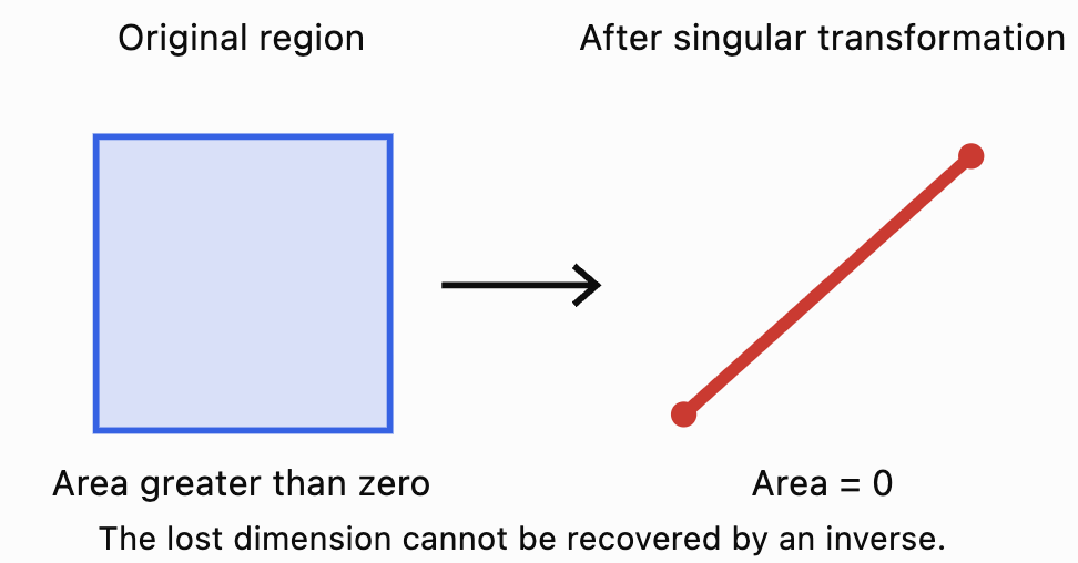
When information is lost in this way, no inverse transformation can uniquely recover every original point.
Singular Matrices and Linear Systems
Consider the system:
2x + 4y = 10
x + 2y = 5
The coefficient matrix is:
Its determinant is:
det(A) = 2(2) − 4(1)
= 0
The matrix is singular.
The first equation is twice the second equation.
Therefore, both equations describe the same line.
There are infinitely many solutions.
Now consider:
2x + 4y = 10
x + 2y = 7
The coefficient matrix is still singular.
However, the equations are inconsistent.
The first equation implies:
x + 2y = 5
while the second requires:
x + 2y = 7
These cannot both be true.
Therefore, the system has no solution.
Important: A zero determinant means that a square linear system does not have a unique solution. It does not tell us whether there are no solutions or infinitely many solutions without examining the equations.
Properties of Inverse Matrices
Inverse matrices follow several useful algebraic rules.
Property 1: Inverse of the inverse
(A⁻¹)⁻¹ = A
Reversing the inverse returns the original matrix.
Property 2: Inverse of a product
(AB)⁻¹ = B⁻¹A⁻¹
The order is reversed.
This is important because matrix multiplication is not generally commutative.
Property 3: Inverse of a transpose
(Aᵀ)⁻¹ = (A⁻¹)ᵀ
Property 4: Inverse of a scalar multiple
For k ≠ 0:
(kA)⁻¹ = (1/k)A⁻¹
provided A is invertible.
Property 5: Identity matrix
I⁻¹ = I
Property 6: Determinant of an inverse
det(A⁻¹) = 1/det(A)
Property 7: Inverse of a power
For a positive integer n:
(Aⁿ)⁻¹ = (A⁻¹)ⁿ
These properties are useful when simplifying complex matrix expressions.
Inverse Matrices and Geometric Transformations
Matrices can represent transformations of points in the coordinate plane.
Inverse matrices reverse these transformations.
Worked Example 9: Reversing a Stretch
Consider:
This transformation stretches x-coordinates by a factor of 2 and y-coordinates by a factor of 3.
For the point:
P(2, 4)
The transformed point is:
The new point is:
P′(4, 12)
To reverse the transformation, calculate the inverse.
Apply the inverse to P′:
The original point has been recovered.
Worked Example 10: Reversing a Rotation
A counterclockwise rotation through 90° is represented by:
The inverse is:
The inverse represents a clockwise rotation through 90°.
If the original point is:
P(3, 2)
the counterclockwise rotation produces:
P′(−2, 3)
Applying R⁻¹ returns:
P(3, 2)
This demonstrates how inverse matrices can undo geometric transformations.
Practical Applications of Inverse Matrices
Application 1: Business and Production Planning
A factory produces two products, A and B.
Each unit of Product A requires:
-
2 hours of machine time.
-
1 hour of labour.
Each unit of Product B requires:
-
1 hour of machine time.
-
3 hours of labour.
The factory has:
-
100 machine hours.
-
120 labour hours.
Let:
x = units of Product A
y = units of Product B
The equations are:
2x + y = 100
x + 3y = 120
Write:
The determinant is:
det(A) = 2(3) − 1(1)
= 5
The inverse is:
Calculate:
Therefore:
The factory should produce 36 units of Product A and 28 units of Product B to use exactly the available machine and labour hours.
Application 2: Recovering Original Data
Suppose two original measurements, x and y, are combined into new measurements:
u = 2x + y
v = x + y
This can be represented as:
If:
u = 11
v = 7
we can recover the original measurements using the inverse.
Therefore:
The original measurements were:
x = 4, y = 3
This type of calculation appears in signal processing and scientific measurement systems.
Application 3: Computer Graphics
Inverse matrices are used in computer graphics to reverse transformations.
For example, a point may be transformed from an object's local coordinate system into a world coordinate system.
An inverse transformation can recover its original local coordinates.
Applications include:
-
Video game graphics
-
Computer animation
-
3D modelling
-
Camera positioning
-
Robotics
-
Engineering simulations
Choosing the Best Method for Finding an Inverse
|
Matrix type |
Recommended method |
|---|---|
|
2 × 2 matrix |
Direct inverse formula |
|
Simple 3 × 3 matrix |
Gauss–Jordan elimination |
|
Larger square matrix |
Row reduction or computational methods |
|
Diagonal matrix |
Take reciprocals of nonzero diagonal elements |
|
Identity matrix |
The inverse is itself |
|
Singular matrix |
No inverse exists |
For a diagonal matrix:
the inverse is:
This works because the diagonal entries are nonzero.
Common Mistakes
Mistake 1: Assuming every matrix has an inverse
Only square matrices with nonzero determinants have ordinary two-sided inverses.
Mistake 2: Dividing every element by the determinant without rearranging the matrix
For a 2 × 2 inverse, the diagonal entries must be exchanged and the off-diagonal signs changed before multiplying by 1/det(A).
Mistake 3: Confusing A⁻¹ with 1/A
Matrix inversion is not element-by-element division.
Mistake 4: Forgetting to check the determinant
If det(A) = 0, the inverse does not exist.
Mistake 5: Making sign errors
Negative signs in the inverse formula must be handled carefully.
Mistake 6: Multiplying matrices in the wrong order
For AX = B:
X = A⁻¹B
not BA⁻¹.
Mistake 7: Assuming AB = BA
Matrix multiplication is generally not commutative.
Mistake 8: Forgetting to verify an inverse
Multiplying A by A⁻¹ should produce the identity matrix.
Mistake 9: Performing row operations on only one side of an augmented matrix
In Gauss–Jordan elimination, every row operation must be applied to the entire augmented matrix.
Mistake 10: Assuming a singular system always has no solution
A singular coefficient matrix may correspond to no solutions or infinitely many solutions.
Mistake 11: Rounding too early
Premature rounding can introduce errors, especially when the determinant is small.
Mistake 12: Forgetting the context of a solution
A mathematical result should be interpreted in the practical situation being modelled.
Key Terms
-
Inverse Matrix: Matrix that reverses the effect of multiplication by an invertible matrix.
-
Invertible Matrix: Square matrix possessing a multiplicative inverse.
-
Identity Matrix: Square matrix with 1 on the main diagonal and 0 elsewhere.
-
Determinant: Scalar value used to determine whether a square matrix is invertible.
-
Singular Matrix: Square matrix with determinant zero.
-
Nonsingular Matrix: Square matrix with nonzero determinant.
-
Matrix Multiplication: Operation combining rows and columns through products and sums.
-
Coefficient Matrix: Matrix containing coefficients of a linear system.
-
Matrix Equation: Equation involving matrices.
-
Augmented Matrix: Matrix formed by placing matrices side by side for row reduction.
-
Elementary Row Operation: Permitted operation used to transform matrix rows.
-
Gauss–Jordan Elimination: Method of row reduction used to solve systems and calculate inverses.
-
Pivot: Leading nonzero element used during row reduction.
-
Row Reduction: Process of simplifying a matrix using elementary row operations.
-
Adjugate Matrix: Transpose of the cofactor matrix.
-
Cofactor: Signed minor associated with a matrix element.
-
Linear Transformation: Mapping represented by matrix multiplication.
-
Inverse Transformation: Transformation that reverses an original transformation.
-
Linear Dependence: Relationship in which one row or column can be expressed using others.
-
Unique Solution: Exactly one solution to a system of equations.
-
Inconsistent System: System with no solutions.
-
Dependent System: System with infinitely many solutions when consistent.
-
Scalar: Single number.
-
Transpose: Matrix formed by interchanging rows and columns.
-
Diagonal Matrix: Square matrix whose off-diagonal entries are zero.
Key Takeaways
-
An inverse matrix reverses the effect of an invertible matrix.
-
The defining property is AA⁻¹ = A⁻¹A = I.
-
Only square matrices with nonzero determinants have ordinary inverses.
-
The inverse of a 2 × 2 matrix can be calculated using a standard formula.
-
The determinant must be checked before calculating an inverse.
-
Inverse matrices can be verified through matrix multiplication.
-
Gauss–Jordan elimination can calculate inverses of larger matrices.
-
Matrix equations of the form AX = B can be solved using X = A⁻¹B.
-
Matrix multiplication order matters.
-
Singular matrices have determinant zero and no inverse.
-
A singular coefficient matrix cannot produce a unique solution to a square linear system.
-
Inverse matrices can reverse geometric transformations.
-
Inverse matrices are useful in business, science, engineering, and computer graphics.
-
In practical problems, solutions must be interpreted in context.
Check Your Understanding
Questions
Question 1: Invertibility
Determine whether the matrix is invertible:
Question 2: Finding an Inverse
Find:
for:
Question 3: Negative Determinant
Find the inverse of:
Question 4: Singular Matrix
Explain why:
has no inverse.
Question 5: Verification
Verify whether:
is the inverse of:
Question 6: Matrix Equation
Solve:
AX = B
where:
Question 7: Linear System
Solve using matrix inverses:
3x + y = 11
x + y = 5
Question 8: Diagonal Matrix
Find the inverse of:
Question 9: Inverse Properties
If det(A) = 5, calculate det(A⁻¹).
Question 10: Product of Inverses
Simplify:
(AB)⁻¹
Question 11: Unknown Matrix Element
Find k so that:
is singular.
Question 12: Geometric Transformation
A transformation doubles x-coordinates and triples y-coordinates.
Write the transformation matrix and its inverse.
Question 13: Three-Variable System
Use the inverse:
to solve:
Question 14: Business Application
A factory makes two products.
Product A requires 2 hours of machine time and 1 hour of labour.
Product B requires 1 hour of machine time and 2 hours of labour.
The factory has 80 machine hours and 70 labour hours.
Use inverse matrices to determine the number of units of each product.
Question 15: Integrated Challenge
Given:
a) Calculate det(A).
b) Determine whether A is invertible.
c) Find A⁻¹.
d) Verify the inverse.
e) Solve:
Fully Worked Answers
Answer 1: Invertibility
det(A) = 3(4) − 1(2)
= 12 − 2
= 10
Since det(A) ≠ 0:
Answer: A is invertible.
Answer 2: Finding an Inverse
det(A) = 2(1) − 1(1)
= 1
Apply the inverse formula:
Answer 3: Negative Determinant
det(B) = 1(4) − 3(2)
= 4 − 6
= −2
Therefore:
Answer 4: Singular Matrix
det(C) = 2(3) − 6(1)
= 6 − 6
= 0
Therefore, C is singular.
Answer: The matrix has no inverse because its determinant is zero.
Answer 5: Verification
Given:
Calculate AB:
Since AB = I and both matrices are square of the same order:
Answer: B is the inverse of A.
Answer 6: Matrix Equation
Given:
The inverse is:
Calculate:
Answer: x = 4, y = 1
Answer 7: Linear System
Equations:
3x + y = 11
x + y = 5
Coefficient matrix:
det(A) = 3(1) − 1(1)
= 2
Inverse:
Calculate:
Answer: x = 3, y = 2
Answer 8: Diagonal Matrix
Take the reciprocal of each diagonal element:
Answer 9: Inverse Properties
Given:
det(A) = 5
Use:
det(A⁻¹) = 1/det(A)
Therefore:
Answer: det(A⁻¹) = 1/5
Answer 10: Product of Inverses
The inverse of a product reverses the multiplication order.
This assumes both A and B are invertible square matrices of the same order.
Answer 11: Unknown Matrix Element
For A to be singular:
det(A) = 0
6k − 2(3) = 0
6k − 6 = 0
6k = 6
Answer: k = 1
Answer 12: Geometric Transformation
Doubling x-coordinates and tripling y-coordinates gives:
The inverse reverses these stretches:
Answer 13: Three-Variable System
Given:
and:
Calculate:
First element:
6 − 8 + 5 = 3
Second element:
8 − 5 = 3
Third element:
5
Therefore:
Answer 14: Business Application
Let:
x = units of Product A
y = units of Product B
Equations:
2x + y = 80
x + 2y = 70
Write:
Calculate the determinant:
det(A) = 2(2) − 1(1)
= 3
The inverse is:
Calculate:
Answer: 30 units of Product A and 20 units of Product B.
Answer 15: Integrated Challenge
Given:
Part a: Determinant
det(A) = 5(1) − 2(3)
= 5 − 6
det(A) = −1
Part b: Invertibility
Since det(A) ≠ 0:
A is invertible.
Part c: Find the inverse
Therefore:
Part d: Verify
Top-left:
5(−1) + 2(3) = 1
Top-right:
5(2) + 2(−5) = 0
Bottom-left:
3(−1) + 1(3) = 0
Bottom-right:
3(2) + 1(−5) = 1
Therefore:
The inverse is verified.
Part e: Solve AX = B
First element:
−19 + 22 = 3
Second element:
57 − 55 = 2
Therefore:
Answer: x = 3, y = 2
Verification:
5(3) + 2(2) = 19
3(3) + 1(2) = 11
Both equations are satisfied.
Final Reflection
Inverse matrices provide a powerful way to reverse matrix transformations and solve systems of linear equations.
The key requirement is invertibility. A square matrix with a nonzero determinant has an inverse, while a singular matrix cannot be inverted because its transformation loses information.
The inverse of a 2 × 2 matrix can be calculated directly using a formula. Larger matrices can be inverted using row reduction, and all inverses can be verified by multiplying them with the original matrix to obtain the identity matrix.
Beyond algebra, inverse matrices are used to reverse geometric transformations, recover original measurements, solve production problems, and analyse scientific and technological systems.
The central idea is that an inverse matrix allows us to reverse a matrix operation, provided the original transformation preserves enough information to be uniquely undone.
5. Systems of Linear Equations
Learning outcomes
- I can represent systems using matrices.
- I can solve systems using matrix methods.
- I can interpret matrix solutions graphically.
- I can compare matrix and algebraic methods.
- I can solve authentic applications involving systems.
Introduction
Many real-world problems involve several unknown quantities connected by multiple equations.
For example:
-
A business may need to determine how many products to manufacture using limited resources.
-
A scientist may need to calculate unknown concentrations in a chemical mixture.
-
An engineer may need to determine forces acting on a structure.
-
A transport company may need to calculate the costs of different delivery methods.
-
A mathematician may need to determine where two or more lines intersect.
These situations can often be represented using systems of linear equations.
A system of linear equations is a collection of two or more linear equations involving the same variables. The goal is to find values that satisfy every equation simultaneously.
Consider:
2x + y = 7
x − y = 2
Solving the system gives:
x = 3, y = 1
We can verify this by substituting into both equations:
2(3) + 1 = 7
3 − 1 = 2
Both equations are satisfied.
Although systems can be solved using substitution, elimination, or graphing, matrices provide a systematic and powerful alternative.
Matrix methods become particularly valuable when solving larger systems containing three or more unknowns.
In this lesson, we will investigate how systems are represented using matrices, how matrix methods are used to find solutions, how solutions are interpreted graphically, and how these techniques apply to authentic mathematical problems.
Understanding Systems of Linear Equations
A linear equation is an equation in which each variable appears only to the first power and variables are not multiplied together.
Examples include:
2x + 3y = 12
4x − y = 7
x + 2y + 3z = 15
A system of linear equations consists of two or more such equations considered together.
Systems with two unknowns
A general system of two linear equations can be written as:
a₁x + b₁y = c₁
a₂x + b₂y = c₂
where:
-
x and y are unknown variables.
-
a₁, a₂, b₁, and b₂ are coefficients.
-
c₁ and c₂ are constants.
A solution is an ordered pair (x, y) satisfying both equations.
Systems with three unknowns
A system involving three unknowns may have the form:
a₁x + b₁y + c₁z = d₁
a₂x + b₂y + c₂z = d₂
a₃x + b₃y + c₃z = d₃
Its solution is an ordered triple:
(x, y, z)
Why use matrices?
Matrices organise the coefficients and constants into a compact structure.
Instead of repeatedly writing entire equations, we can perform operations directly on their numerical coefficients.
This makes it easier to develop systematic procedures and use computational tools.
Representing Systems Using Matrices
Consider the system:
3x + 2y = 16
x − y = 2
We can represent it using three matrices.
Coefficient matrix
The coefficient matrix contains the coefficients of the variables.
Variable matrix
The variable matrix contains the unknown quantities.
Constant matrix
The constant matrix contains the values on the right side of the equations.
The system can now be written as:
or:
Multiplying the matrices on the left gives:
This reproduces the original system.
Visualising the matrix representation
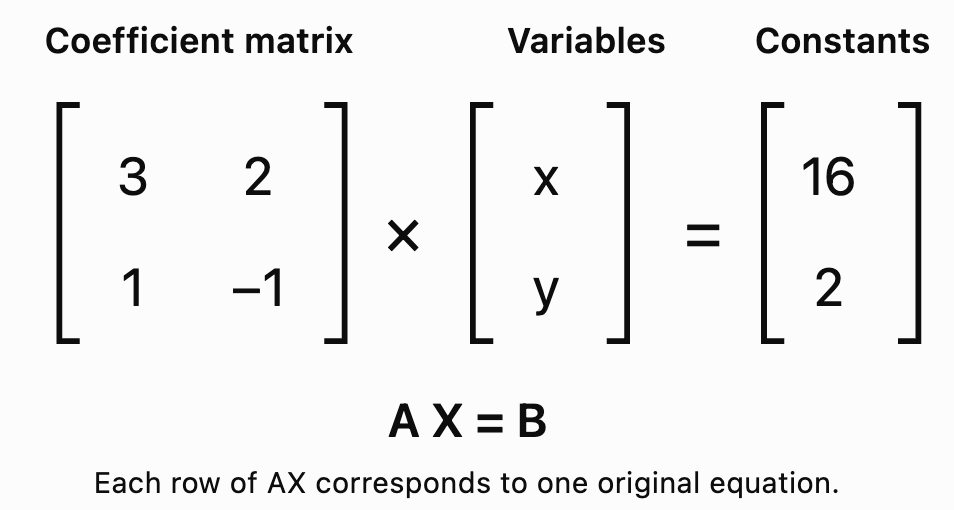
Important rules for constructing matrix equations
-
Keep the variables in the same order in every equation.
-
Include zero coefficients when a variable is missing.
-
Place constants in the correct corresponding rows.
-
Ensure the dimensions are compatible for multiplication.
Worked Example 1: Writing a System in Matrix Form
Write the following system in the form AX = B.
2x + 3y − z = 8
4x − y + 2z = 11
x + 5z = 7
Step 1: Identify the variables.
The variables are:
x, y, z
Step 2: Arrange the coefficients.
Notice that the third equation does not contain y.
Therefore, its y-coefficient is zero.
The coefficient matrix is:
Step 3: Construct the variable matrix.
Step 4: Construct the constant matrix.
Therefore:
The dimensions are:
A: 3 × 3
X: 3 × 1
B: 3 × 1
The multiplication is valid because:
(3 × 3)(3 × 1) = 3 × 1
Augmented Matrices
An augmented matrix combines the coefficient matrix and the constant matrix into one arrangement.
For the system:
3x + 2y = 16
x − y = 2
the augmented matrix is:
The vertical line separates the coefficients from the constants.
An augmented matrix is especially useful for solving systems through row operations.
Why augmented matrices are useful
They allow us to:
-
Organise all the numerical information in one place.
-
Perform elimination systematically.
-
Solve systems with several variables.
-
Identify systems with no solution.
-
Identify systems with infinitely many solutions.
Solving Systems Using Gaussian Elimination
Gaussian elimination is a matrix method that uses elementary row operations to simplify a system.
The goal is to transform the augmented matrix into row echelon form, from which the variables can be found using back-substitution.
Elementary row operations
There are three allowed operations.
-
Interchange two rows.
-
Multiply a row by a nonzero number.
-
Add a multiple of one row to another row.
These operations preserve the solution set of the system.
Worked Example 2: Gaussian Elimination
Solve:
2x + y = 7
x − y = 2
Step 1: Construct the augmented matrix.
Step 2: Swap the rows.
This places a coefficient of 1 in the top-left position.
R₁ ↔ R₂
Step 3: Eliminate the x-coefficient in row 2.
R₂ → R₂ − 2R₁
Step 4: Solve for y.
The second row represents:
3y = 3
Therefore:
y = 1
Step 5: Substitute into the first equation.
x − y = 2
x − 1 = 2
x = 3
Therefore:
Verification
2(3) + 1 = 7
3 − 1 = 2
Both equations are satisfied.
Gauss–Jordan Elimination
Gauss–Jordan elimination extends Gaussian elimination by continuing the row operations until the coefficient portion is in reduced row echelon form.
For a system with a unique solution, the final matrix has the form:
The solution can be read directly from the final column.
Worked Example 3: Gauss–Jordan Elimination
Solve:
2x + y = 9
x + 2y = 6
Step 1: Write the augmented matrix.
Step 2: Swap the rows.
Step 3: Eliminate the 2 below the first pivot.
R₂ → R₂ − 2R₁
Step 4: Divide row 2 by −3.
R₂ → −(1/3)R₂
Step 5: Eliminate the 2 above the second pivot.
R₁ → R₁ − 2R₂
Therefore:
This method is particularly useful because it provides the solution without requiring a separate back-substitution stage.
Solving Systems Using Inverse Matrices
A system can be written as:
AX = B
If A is square and invertible:
This method is useful when the coefficient matrix has a nonzero determinant.
Worked Example 4: Solving with an Inverse Matrix
Solve:
3x + y = 11
2x + y = 8
Step 1: Write the system in matrix form.
Step 2: Calculate the determinant.
det(A) = 3(1) − 1(2)
= 1
The matrix is invertible.
Step 3: Find the inverse.
Step 4: Calculate X.
First element:
11 − 8 = 3
Second element:
−22 + 24 = 2
Therefore:
x = 3, y = 2
Verification
3(3) + 2 = 11
2(3) + 2 = 8
Both equations are satisfied.
Solving Systems Using Cramer's Rule
Cramer's Rule uses determinants to solve square systems with a nonzero coefficient determinant.
For:
ax + by = e
cx + dy = f
define:
If D ≠ 0:
Worked Example 5: Cramer's Rule
Solve:
2x + 3y = 13
x + y = 5
Step 1: Calculate D.
D = 2(1) − 3(1)
= −1
Step 2: Calculate Dₓ.
Dₓ = 13(1) − 3(5)
= −2
Step 3: Calculate Dᵧ.
Dᵧ = 2(5) − 13(1)
= −3
Step 4: Calculate x and y.
x = Dₓ/D = (−2)/(−1) = 2
y = Dᵧ/D = (−3)/(−1) = 3
Therefore:
Solving Systems with Three Unknowns
Matrix methods are particularly valuable for systems containing three or more variables.
Consider:
x + y + z = 6
2x − y + z = 3
x + 2y − z = 2
Worked Example 6: Three-Variable Gaussian Elimination
Step 1: Write the augmented matrix.
Step 2: Eliminate x from rows 2 and 3.
R₂ → R₂ − 2R₁
R₃ → R₃ − R₁
Step 3: Swap rows 2 and 3.
Step 4: Eliminate y from row 3.
R₃ → R₃ + 3R₂
Step 5: Solve for z.
−7z = −21
z = 3
Step 6: Solve for y.
From row 2:
y − 2z = −4
y − 6 = −4
y = 2
Step 7: Solve for x.
From row 1:
x + y + z = 6
x + 2 + 3 = 6
x = 1
Therefore:
Verification
First equation:
1 + 2 + 3 = 6
Second equation:
2(1) − 2 + 3 = 3
Third equation:
1 + 2(2) − 3 = 2
All three equations are satisfied.
Graphical Interpretation of Linear Systems
Every linear equation in two variables represents a straight line.
When two equations are considered together, their solutions correspond to the intersection points of the lines.
There are three main possibilities.
Case 1: One unique solution
Two nonparallel lines intersect at exactly one point.
For example:
y = 2x + 1
y = −x + 7
Set the equations equal:
2x + 1 = −x + 7
3x = 6
x = 2
Substitute:
y = 2(2) + 1 = 5
The intersection is:
(2, 5)
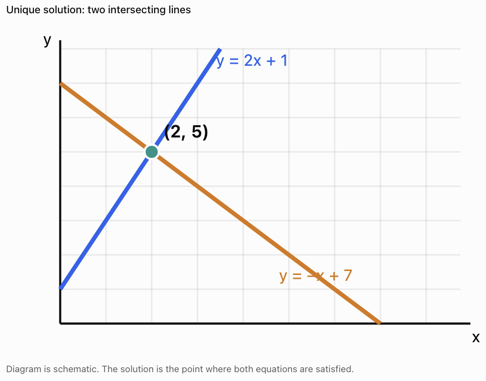
The coefficient determinant is nonzero, so the system has a unique solution.
Case 2: No solution
Consider:
y = 2x + 1
y = 2x − 3
Both lines have the same gradient but different y-intercepts.
They are parallel and never intersect.
Therefore:
The system has no solution.
The coefficient matrix has determinant zero.
Case 3: Infinitely many solutions
Consider:
2x + y = 6
4x + 2y = 12
The second equation is twice the first.
Both equations describe the same line.
Therefore:
The system has infinitely many solutions.
The coefficient matrix again has determinant zero.
Comparing the three cases
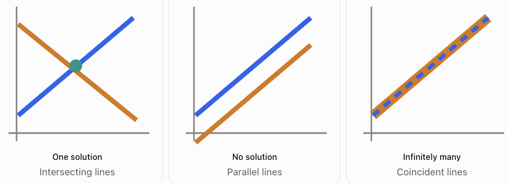
Matrix Interpretation of Different Solution Types
When using row reduction, the final augmented matrix reveals the nature of the system.
Unique solution
This represents:
x = 3
y = 2
There is one unique solution.
No solution
The second row represents:
0x + 0y = 3
or:
0 = 3
This is impossible.
Therefore, the system is inconsistent and has no solution.
Infinitely many solutions
The second row represents:
0 = 0
This provides no new restriction.
The first row gives:
x + 2y = 5
Let:
y = t
Then:
x = 5 − 2t
Therefore, the solutions can be written as:
(x, y) = (5 − 2t, t)
where t can be any real number.
This describes infinitely many solutions.
For a general system, the number of free variables determines the number of parameters needed to describe the solution set.
Systems of Three Equations: Graphical Interpretation
In three dimensions, a linear equation generally represents a plane rather than a line.
Three planes can:
-
Intersect at one point.
-
Share a common line.
-
Coincide.
-
Have no common intersection.
A unique solution corresponds to one point where all three planes meet.
A system with infinitely many solutions may have a common line or plane of solutions.
A system with no solution has no point satisfying all three equations simultaneously.
For a square 3 × 3 coefficient matrix:
-
det(A) ≠ 0 guarantees one unique solution.
-
det(A) = 0 means the system has no unique solution.
The second case must be investigated further to determine whether there are no solutions or infinitely many solutions.
Comparing Matrix and Algebraic Methods
Systems can be solved using several approaches.
|
Method |
Main idea |
Most useful when |
|---|---|---|
|
Graphing |
Find intersections |
Visual interpretation or approximate solutions |
|
Substitution |
Isolate and replace a variable |
A variable is easy to isolate |
|
Elimination |
Add or subtract equations |
Coefficients can be eliminated easily |
|
Gaussian elimination |
Use matrix row operations |
Larger systems with several variables |
|
Gauss–Jordan elimination |
Reduce to a direct solution form |
Systematic solution and classification |
|
Inverse matrices |
Calculate X = A⁻¹B |
Square, invertible coefficient matrix |
|
Cramer's Rule |
Use determinants |
Small square systems with nonzero determinant |
Example: Comparing methods
Consider:
x + y = 7
x − y = 1
Algebraic elimination
Add the equations:
2x = 8
x = 4
Then:
y = 3
Matrix method
R₂ → R₂ − R₁
Therefore:
y = 3
x = 4
Both methods produce the same solution.
For a small system, algebraic elimination may be faster. For a system with many variables, matrix methods provide a more organised and scalable procedure.
Real-World Application 1: Ticket Sales
A school sells adult and student tickets for a concert.
Adult tickets cost $12.
Student tickets cost $7.
A total of 150 tickets are sold.
The total revenue is $1,350.
How many adult and student tickets were sold?
Step 1: Define variables
Let:
x = number of adult tickets
y = number of student tickets
Step 2: Construct equations
Total tickets:
x + y = 150
Total revenue:
12x + 7y = 1350
Step 3: Write the matrix equation
Step 4: Solve
The determinant is:
D = 1(7) − 1(12)
= −5
The inverse is:
Multiply:
First component:
(1050 − 1350)/(−5) = 60
Second component:
(−1800 + 1350)/(−5) = 90
Therefore:
60 adult tickets and 90 student tickets were sold.
Verification
60 + 90 = 150
12(60) + 7(90) = 720 + 630 = 1350
Both conditions are satisfied.
Real-World Application 2: Mixture Problems
A laboratory needs 20 litres of a 35% solution.
Two solutions are available:
-
Solution A: 20% concentration.
-
Solution B: 50% concentration.
How many litres of each solution should be mixed?
Step 1: Define variables
x = litres of 20% solution
y = litres of 50% solution
Step 2: Construct equations
Total volume:
x + y = 20
Amount of dissolved substance:
0.20x + 0.50y = 0.35(20)
Therefore:
0.20x + 0.50y = 7
Step 3: Matrix representation
Step 4: Solve by elimination
Multiply the first equation by 0.20:
0.20x + 0.20y = 4
Subtract from the concentration equation:
0.30y = 3
y = 10
Then:
x + 10 = 20
x = 10
Therefore:
10 litres of the 20% solution and 10 litres of the 50% solution are required.
This model assumes volumes are additive and the solutions mix uniformly.
Real-World Application 3: Production Planning
A workshop manufactures tables and chairs.
Each table requires:
-
4 hours of cutting.
-
2 hours of assembly.
Each chair requires:
-
2 hours of cutting.
-
3 hours of assembly.
The workshop has:
-
100 cutting hours.
-
90 assembly hours.
Determine how many tables and chairs can be manufactured if all available hours are used.
Let:
x = number of tables
y = number of chairs
The equations are:
4x + 2y = 100
2x + 3y = 90
The matrix equation is:
The determinant is:
D = 4(3) − 2(2)
= 8
The inverse is:
Calculate:
Therefore:
The workshop can manufacture 15 tables and 20 chairs.
Verification
Cutting:
4(15) + 2(20) = 100
Assembly:
2(15) + 3(20) = 90
The solution satisfies both resource constraints.
Real-World Application 4: Electrical Circuits
In electrical engineering, systems of linear equations are used to calculate unknown currents in circuits.
Kirchhoff's laws produce equations describing relationships between currents and voltages.
For example, suppose two unknown loop currents satisfy:
5I₁ − 2I₂ = 12
−2I₁ + 4I₂ = 6
The matrix equation is:
The determinant is:
D = 5(4) − (−2)(−2)
= 20 − 4
= 16
The inverse is:
Therefore:
Thus:
I₁ = 3.75 A
I₂ = 3.375 A
The currents satisfy the original equations.
This illustrates how matrix methods can solve systems arising in electrical engineering.
Choosing an Efficient Strategy
When solving a system, begin by examining its structure.
If the system has two equations with simple coefficients:
Substitution or elimination may be quickest.
If the system has three or more variables:
Gaussian elimination is often a good choice.
If the coefficient matrix is square and invertible:
Inverse matrices or Cramer's Rule are possible.
If you need to identify whether a system has no solution or infinitely many solutions:
Row reduction is particularly useful.
If a graphical interpretation is important:
Graph the equations to understand the solution geometrically.
If the system is large:
Computational linear algebra methods are usually more efficient than calculating a full inverse explicitly.
Common Mistakes
Mistake 1: Placing coefficients in the wrong columns
Always keep the variables in the same order.
Mistake 2: Forgetting zero coefficients
If an equation does not contain a variable, include a zero in its column.
Mistake 3: Mixing coefficients and constants
The augmented matrix must preserve the correct relationship between equations and constants.
Mistake 4: Performing row operations on only part of the augmented matrix
Every row operation must apply to the entire row, including the constant column.
Mistake 5: Making sign errors during elimination
Subtracting a negative number produces a positive result.
Mistake 6: Using inverse matrices when the determinant is zero
The inverse does not exist for a singular matrix.
Mistake 7: Assuming a zero determinant means no solution
A singular system may have no solutions or infinitely many solutions.
Mistake 8: Confusing Gaussian and Gauss–Jordan elimination
Gaussian elimination typically uses back-substitution; Gauss–Jordan elimination continues to reduced row echelon form.
Mistake 9: Interpreting every system as having one solution
Systems can have one, none, or infinitely many solutions.
Mistake 10: Forgetting to check answers
Substitute solutions into every original equation.
Mistake 11: Using graphing as though it always gives exact values
Graphical solutions may be approximate unless the intersection is known exactly.
Mistake 12: Ignoring real-world constraints
Negative quantities or fractional numbers of indivisible products may not be meaningful.
Key Terms
-
Linear Equation: Equation involving variables only to the first power.
-
System of Linear Equations: Collection of linear equations involving common variables.
-
Simultaneous Solution: Values satisfying all equations in a system.
-
Coefficient: Number multiplying a variable.
-
Constant: Fixed numerical value.
-
Coefficient Matrix: Matrix containing the coefficients of a linear system.
-
Variable Matrix: Column matrix containing the unknown variables.
-
Constant Matrix: Column matrix containing the right-hand-side values.
-
Matrix Equation: Equation expressed using matrices.
-
Augmented Matrix: Matrix combining coefficients and constants.
-
Gaussian Elimination: Method using row operations to reach row echelon form.
-
Gauss–Jordan Elimination: Method using row operations to reach reduced row echelon form.
-
Elementary Row Operation: Allowed operation that preserves the solution set.
-
Pivot: Leading nonzero entry used during row reduction.
-
Row Echelon Form: Matrix form suitable for back-substitution.
-
Reduced Row Echelon Form: Matrix form with leading ones and zeros elsewhere in pivot columns.
-
Back-Substitution: Solving variables from the last equation upward.
-
Inverse Matrix: Matrix reversing the multiplication effect of an invertible matrix.
-
Determinant: Scalar value used to test invertibility of a square matrix.
-
Cramer's Rule: Method solving square linear systems using determinants.
-
Unique Solution: Exactly one solution satisfying the system.
-
Inconsistent System: System with no solution.
-
Dependent System: System containing redundant equations.
-
Independent Equations: Equations contributing independent constraints.
-
Singular Matrix: Square matrix with determinant zero.
-
Free Variable: Variable that can take arbitrary values in a system with infinitely many solutions.
-
Parameter: Symbol used to describe a family of solutions.
-
Intersection Point: Point shared by two or more graphs.
-
Parallel Lines: Lines in a plane that never intersect.
-
Coincident Lines: Lines that occupy exactly the same position.
-
Linear Model: Mathematical representation using linear relationships.
Key Takeaways
-
A system of linear equations contains two or more equations involving common variables.
-
A solution must satisfy every equation simultaneously.
-
Systems can be represented compactly as AX = B.
-
The coefficient matrix contains the variable coefficients.
-
The augmented matrix combines coefficients and constants.
-
Gaussian elimination uses row operations and back-substitution.
-
Gauss–Jordan elimination reduces the system to a form where solutions can be read directly.
-
Inverse matrices solve systems using X = A⁻¹B when A is invertible.
-
Cramer's Rule uses determinants to solve square systems with nonzero determinants.
-
A system can have one solution, no solution, or infinitely many solutions.
-
In two dimensions, solutions correspond to intersections of lines.
-
Parallel distinct lines produce no solution.
-
Coincident lines produce infinitely many solutions.
-
A nonzero determinant guarantees a unique solution for a square system.
-
A zero determinant means a square system does not have a unique solution.
-
Different solving methods are useful in different situations.
-
Matrix methods are especially valuable for larger systems.
-
Real-world applications include business, chemistry, engineering, and electrical circuits.
Check Your Understanding
Questions
Question 1: Matrix Representation
Write the system in matrix form:
2x + 3y = 12
4x − y = 5
Question 2: Augmented Matrix
Construct the augmented matrix for:
x + 2y = 7
3x − y = 8
Question 3: Missing Coefficient
Write the coefficient matrix for:
2x + 3z = 8
x + y − z = 4
3y + 2z = 9
Question 4: Gaussian Elimination
Solve:
x + y = 9
2x − y = 3
Question 5: Gauss–Jordan Elimination
Solve:
2x + y = 8
x + 3y = 9
Question 6: Inverse Matrix Method
Solve using an inverse matrix:
3x + y = 10
x + y = 6
Question 7: Cramer's Rule
Solve:
2x + y = 7
x − y = 2
Question 8: Graphical Interpretation
Determine the number of solutions:
y = 3x + 2
y = 3x − 5
Explain your reasoning.
Question 9: Infinitely Many Solutions
Determine the number of solutions:
2x + 4y = 12
x + 2y = 6
Question 10: Singular Matrix
Determine whether the coefficient matrix of:
3x + 6y = 9
x + 2y = 3
is singular.
Question 11: Three-Variable System
Solve:
x + y + z = 9
x − y + z = 3
2x + y − z = 3
Question 12: Ticket Sales
A cinema sells adult tickets for $15 and student tickets for $10.
A total of 120 tickets are sold.
Revenue is $1,500.
How many of each ticket were sold?
Question 13: Mixture Problem
A laboratory needs 30 litres of a 40% solution.
It has 20% and 50% solutions.
How many litres of each are required?
Question 14: Comparing Methods
Explain why Gaussian elimination may be preferable to graphing for a system with four unknown variables.
Question 15: Integrated Challenge
Consider:
2x + y = 11
3x − 2y = 4
a) Write the matrix equation AX = B.
b) Construct the augmented matrix.
c) Calculate det(A).
d) Solve the system using a matrix method.
e) Explain the graphical meaning of the solution.
f) Verify the solution.
Fully Worked Answers
Answer 1: Matrix Representation
System:
2x + 3y = 12
4x − y = 5
The coefficient matrix is:
The variable matrix is:
The constant matrix is:
Therefore:
Answer 2: Augmented Matrix
System:
x + 2y = 7
3x − y = 8
The augmented matrix is:
Answer 3: Missing Coefficient
System:
2x + 3z = 8
x + y − z = 4
3y + 2z = 9
The missing coefficients are zero.
Therefore:
Answer 4: Gaussian Elimination
System:
x + y = 9
2x − y = 3
Augmented matrix:
R₂ → R₂ − 2R₁
Therefore:
−3y = −15
y = 5
Substitute:
x + 5 = 9
x = 4
Answer: x = 4, y = 5
Answer 5: Gauss–Jordan Elimination
System:
2x + y = 8
x + 3y = 9
Augmented matrix:
Swap rows:
R₂ → R₂ − 2R₁
R₂ → −(1/5)R₂
R₁ → R₁ − 3R₂
Answer: x = 3, y = 2
Answer 6: Inverse Matrix Method
System:
3x + y = 10
x + y = 6
Coefficient matrix:
det(A) = 3(1) − 1(1)
= 2
Inverse:
Calculate:
Answer: x = 2, y = 4
Answer 7: Cramer's Rule
System:
2x + y = 7
x − y = 2
Calculate:
D = 2(−1) − 1(1)
= −3
Dₓ = 7(−1) − 1(2)
= −9
Dᵧ = 2(2) − 7(1)
= −3
Therefore:
x = Dₓ/D = (−9)/(−3) = 3
y = Dᵧ/D = (−3)/(−3) = 1
Answer: x = 3, y = 1
Answer 8: Graphical Interpretation
Equations:
y = 3x + 2
y = 3x − 5
Both lines have gradient 3.
However, their y-intercepts are different.
Therefore, they are distinct parallel lines.
Answer: No solution.
Answer 9: Infinitely Many Solutions
Equations:
2x + 4y = 12
x + 2y = 6
Multiply the second equation by 2:
2x + 4y = 12
This is identical to the first equation.
Therefore, both equations represent the same line.
Answer: Infinitely many solutions.
Answer 10: Singular Matrix
Coefficient matrix:
det(A) = 3(2) − 6(1)
= 6 − 6
= 0
Therefore:
Answer: The coefficient matrix is singular.
The equations are also consistent because the first is three times the second, so the system has infinitely many solutions.
Answer 11: Three-Variable System
System:
x + y + z = 9
x − y + z = 3
2x + y − z = 3
Subtract the second equation from the first:
2y = 6
y = 3
Substitute into the first equation:
x + z = 6
Substitute y = 3 into the third equation:
2x + 3 − z = 3
2x − z = 0
Therefore:
z = 2x
Substitute into x + z = 6:
x + 2x = 6
3x = 6
x = 2
Then:
z = 4
Answer: x = 2, y = 3, z = 4
Answer 12: Ticket Sales
Let:
x = adult tickets
y = student tickets
Equations:
x + y = 120
15x + 10y = 1500
Multiply the first equation by 10:
10x + 10y = 1200
Subtract:
5x = 300
x = 60
Then:
y = 120 − 60
y = 60
Answer: 60 adult tickets and 60 student tickets.
Verification:
15(60) + 10(60) = 1500
Answer 13: Mixture Problem
Let:
x = litres of 20% solution
y = litres of 50% solution
Total volume:
x + y = 30
Concentration equation:
0.20x + 0.50y = 0.40(30)
0.20x + 0.50y = 12
Multiply the volume equation by 0.20:
0.20x + 0.20y = 6
Subtract:
0.30y = 6
y = 20
Then:
x = 30 − 20
x = 10
Answer: 10 litres of 20% solution and 20 litres of 50% solution.
Answer 14: Comparing Methods
Gaussian elimination is preferable for a system with four unknowns because:
-
It provides a systematic algebraic procedure.
-
It can produce exact solutions.
-
It avoids the difficulty of graphing equations in four dimensions.
-
It can identify inconsistent or dependent systems.
-
It extends naturally to larger systems.
Answer: Gaussian elimination is generally more practical and precise for systems involving several variables.
Answer 15: Integrated Challenge
System:
2x + y = 11
3x − 2y = 4
Part a: Matrix equation
Part b: Augmented matrix
Part c: Determinant
det(A) = 2(−2) − 1(3)
= −4 − 3
det(A) = −7
Since the determinant is nonzero, the system has one unique solution.
Part d: Solve using the inverse matrix
Calculate:
Therefore:
Part e: Graphical interpretation
The two lines intersect at exactly one point:
(26/7, 25/7)
This is the unique solution.
Part f: Verification
First equation:
2(26/7) + 25/7
= 52/7 + 25/7
= 77/7
= 11
Second equation:
3(26/7) − 2(25/7)
= 78/7 − 50/7
= 28/7
= 4
Both equations are satisfied.
Final Reflection
Systems of linear equations provide a mathematical framework for understanding relationships involving several unknown quantities.
Matrix notation allows us to represent these relationships efficiently and solve them using systematic procedures.
Gaussian elimination, Gauss–Jordan elimination, inverse matrices, and Cramer's Rule all provide ways to solve systems, but each method has different advantages.
Graphical interpretation helps us understand why systems may have one solution, no solution, or infinitely many solutions.
The greatest value of these methods becomes clear when they are applied to real-world situations. Business planning, scientific mixtures, engineering systems, and electrical circuits can all be represented using systems of linear equations.
The central idea is that matrix methods transform collections of linear equations into organised numerical structures that can be analysed, solved, and interpreted efficiently.