Advanced Exponential and Logarithmic Models
4. Logistic Growth Models
Learning outcomes
- I can explain logistic growth.
- I can distinguish logistic and exponential growth.
- I can interpret carrying capacity.
- I can analyse logistic graphs.
- I can model real-world population growth.
Introduction
Imagine introducing a small population of rabbits into a large grassland. At first, food is plentiful, space is available, and the rabbits reproduce rapidly. As the population increases, however, more rabbits compete for the same resources.
Eventually, the population may become so large that the environment cannot support continued rapid growth.
This situation illustrates an important limitation of exponential growth: real populations cannot usually grow exponentially forever.
Exponential models assume that a population maintains a constant proportional growth rate. In reality, populations are influenced by food availability, water, space, competition, disease, and other environmental factors.
A logistic growth model accounts for these limitations by allowing population growth to slow as the population approaches the maximum level that the environment can sustain.
Logistic models produce a characteristic S-shaped curve and are widely used in ecology, population biology, epidemiology, resource management, and mathematical modelling.
In this lesson, we will explore the mathematical structure of logistic growth, compare it with exponential growth, interpret carrying capacity, analyse logistic graphs, and develop models for real-world populations.
What Is Logistic Growth?
Logistic growth is a pattern of population change in which growth is initially approximately exponential but gradually slows as the population approaches a limiting value.
This limiting value is called the carrying capacity.
Logistic growth typically occurs in three stages.
-
Early growth: The population is relatively small, resources are abundant, and growth accelerates.
-
Rapid growth: The population increases quickly, but competition for resources becomes increasingly important.
-
Slowing growth: Population growth decreases as the population approaches carrying capacity.
For an initial population below carrying capacity, the resulting graph is often S-shaped, also called a sigmoid curve.
The characteristic logistic growth curve
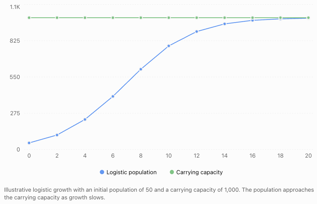
The population does not suddenly stop growing when it reaches a particular size. Instead, its growth rate gradually decreases as it approaches the limiting value.
Exponential Growth Versus Logistic Growth
Both exponential and logistic models describe population growth, but they make different assumptions.
Exponential growth
The exponential growth model is:
P(t) = P₀eʳᵗ
Where:
-
P(t) = population at time t
-
P₀ = initial population
-
r = constant continuous relative growth rate
-
t = time
The model assumes that the population's relative growth rate remains constant.
Consequently, the population grows without bound when r > 0.
Logistic growth
The logistic model modifies exponential growth by accounting for limited resources.
Its relative growth rate decreases as the population approaches carrying capacity.
|
Feature |
Exponential growth |
Logistic growth |
|---|---|---|
|
Graph shape |
J-shaped |
Usually S-shaped |
|
Resource availability |
Assumed unlimited or nonlimiting |
Limited |
|
Relative growth rate |
Constant |
Decreases as population increases |
|
Carrying capacity |
Not included |
Included |
|
Long-term behaviour |
Unlimited growth for r > 0 |
Approaches a limiting population |
|
Typical application |
Early population growth |
Growth under resource constraints |
Comparing the two models
Consider a population that begins with 50 organisms.
Suppose the exponential model has a continuous growth rate of 40% per year, while the logistic model has the same intrinsic growth parameter and a carrying capacity of 1,000.
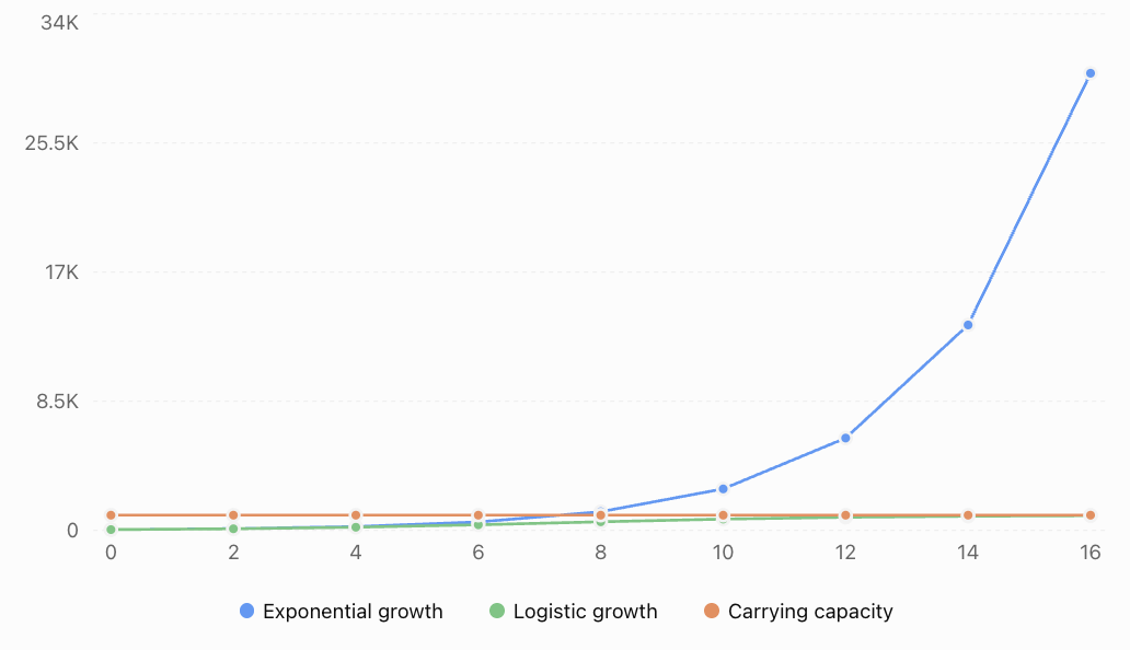
Initially, the models produce relatively similar predictions because the population is small compared with carrying capacity.
Over time, however, the exponential model continues increasing rapidly while the logistic model begins to level off.
The central difference is that logistic growth incorporates density-dependent limitations on population growth.
Carrying Capacity
The carrying capacity, represented by K, is the population size that an environment can sustain in the long term under the conditions assumed by the model.
Carrying capacity depends on factors such as:
-
Food availability.
-
Water availability.
-
Living space.
-
Competition.
-
Disease and predation.
-
Availability of shelter.
-
Environmental conditions.
For example, a lake may support approximately 5,000 fish under a particular set of ecological conditions.
If the population is much smaller than 5,000, resources may be plentiful and the population may increase.
As the population approaches 5,000, competition becomes stronger and population growth slows.
If the population temporarily exceeds carrying capacity, the logistic model predicts a decrease toward K.
Is carrying capacity always constant?
No.
In a basic logistic model, K is assumed to remain constant.
In real ecosystems, carrying capacity may change because of droughts, climate changes, habitat destruction, seasonal conditions, or changes in food availability.
Therefore, carrying capacity should be understood as a model parameter representing environmental limits under particular conditions, not necessarily a permanent population maximum.
The Logistic Growth Equation
The logistic growth model can be expressed as a differential equation.
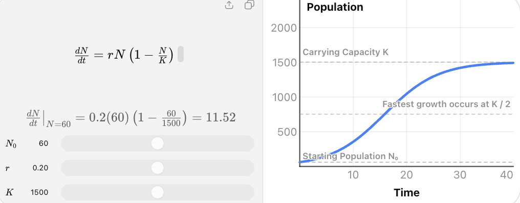
Where:
-
N = population size.
-
t = time.
-
r = intrinsic per-capita growth rate.
-
K = carrying capacity.
-
dN/dt = instantaneous rate of population change.
The expression (1 − N/K) is called the density-dependent limiting factor.
It reduces the growth rate as the population approaches carrying capacity.
Understanding the limiting factor
Suppose K = 1,000.
|
Population N |
N/K |
1 − N/K |
Interpretation |
|---|---|---|---|
|
100 |
0.10 |
0.90 |
Growth is only slightly reduced |
|
250 |
0.25 |
0.75 |
Some resource limitation |
|
500 |
0.50 |
0.50 |
Stronger limitation |
|
750 |
0.75 |
0.25 |
Growth is considerably reduced |
|
900 |
0.90 |
0.10 |
Growth is slow |
|
1,000 |
1.00 |
0 |
No net growth |
|
1,100 |
1.10 |
−0.10 |
Population decreases |
This table illustrates why logistic growth differs from exponential growth.
The population's instantaneous growth rate depends on both its current size and its proximity to carrying capacity.
The Logistic Population Function
The differential equation has a solution of the form:
Where:
-
P(t) = population at time t.
-
K = carrying capacity.
-
r = intrinsic growth parameter.
-
A = constant determined by the initial population.
-
t = time.
If the initial population is P₀, then:
An equivalent form is:
This equation is particularly useful because it allows us to calculate the population at any specified time.
Understanding the parameters
K: Carrying capacity
Determines the long-term limiting population.
P₀: Initial population
Determines the population at t = 0.
r: Intrinsic growth parameter
Controls the time scale of population growth. A larger positive r produces a faster approach toward carrying capacity, all else being equal.
A: Initial-condition constant
Determines how the curve is positioned relative to time zero.
For a population beginning below carrying capacity, A is positive.
Worked Example 1: Developing a Logistic Model
A nature reserve introduces 100 deer into an environment with a carrying capacity of 1,000 deer.
The intrinsic growth parameter is r = 0.4 per year.
Develop a logistic population model.
Step 1: Identify the parameters.
K = 1000
P₀ = 100
r = 0.4
Step 2: Calculate A.
Step 3: Write the model.
This model predicts the deer population t years after introduction.
Checking the initial population
At t = 0:
The model correctly reproduces the initial population.
Worked Example 2: Predicting Population Size
Using the deer population model:
Calculate the population after 5 years.
Step 1: Substitute t = 5.
Step 2: Simplify the exponent.
Step 3: Evaluate the exponential term.
The predicted deer population after five years is approximately 451.
Further predictions
|
Time (years) |
Predicted population |
|---|---|
|
0 |
100 |
|
2 |
198 |
|
4 |
355 |
|
5 |
451 |
|
6 |
551 |
|
8 |
732 |
|
10 |
858 |
|
12 |
931 |
|
15 |
978 |
|
20 |
997 |
The population increases rapidly at first, then gradually approaches 1,000.
Analysing Logistic Graphs
A logistic graph provides information about initial population, growth rate, carrying capacity, and long-term behaviour.
The three main regions
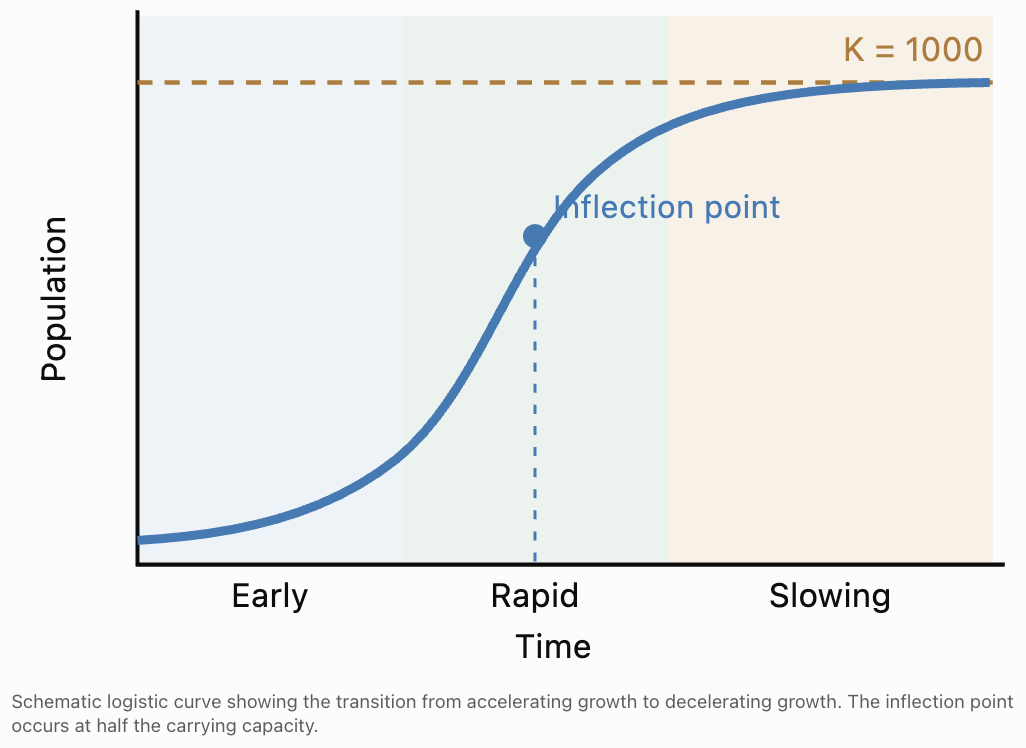
Region 1: Early growth
When the population is small compared with K, resource limitations are relatively weak.
The population increases and its absolute growth rate accelerates.
Region 2: Rapid growth
The population grows quickly.
However, as resource competition increases, the growth rate eventually reaches its maximum and then begins to decline.
Region 3: Slowing growth
As the population approaches carrying capacity, the growth rate decreases toward zero.
The graph becomes nearly horizontal.
The Inflection Point
The inflection point is where the logistic graph changes from curving upward to curving downward.
For the standard logistic growth model with r > 0:
This is also the population at which the instantaneous absolute growth rate is greatest.
For a carrying capacity of 1,000:
The maximum growth rate occurs when the population reaches 500.
Why does maximum growth occur at half the carrying capacity?
At low population sizes, there are relatively few organisms reproducing.
At high population sizes, resource limitations strongly reduce growth.
At half the carrying capacity, the balance between population size and resource availability produces the maximum net growth rate in the standard model.
The maximum instantaneous growth rate is:
Worked Example 3: Maximum Growth Rate
A population has:
K = 2,000
r = 0.3 per year
Calculate the population at maximum growth and the maximum instantaneous growth rate.
Step 1: Find the population at the inflection point.
Step 2: Calculate the maximum growth rate.
The population grows most rapidly when it reaches 1,000 organisms, at an instantaneous rate of 150 organisms per year.
Finding the Time at Which a Population Reaches a Target
Logistic equations can be rearranged using natural logarithms.
Starting with:
Multiply both sides by the denominator:
Divide by P:
Subtract 1:
Divide by A:
Take natural logarithms:
Therefore:
For a population starting below K, this formula applies to target populations between 0 and K.
Worked Example 4: Time to Reach Half the Carrying Capacity
Return to the deer population model:
Find when the population reaches 500 deer.
Step 1: Substitute P(t) = 500.
Step 2: Rearrange.
Step 3: Take natural logarithms.
Since ln(1/9) = −ln(9):
Step 4: Solve.
The deer population reaches 500 after approximately 5.49 years.
At this point, its instantaneous growth rate is greatest.
Worked Example 5: Time to Reach 90% of Carrying Capacity
Using the same model, find when the population reaches 900 deer.
Rearrange:
Take natural logarithms:
The population reaches 90% of carrying capacity after approximately 10.99 years.
Notice that it takes considerably longer to approach the final limiting population than to pass through the middle portion of the curve.
Estimating a Logistic Model from Data
Sometimes the carrying capacity and initial population are known, but the growth parameter r must be estimated.
Suppose a fish population is modelled by:
Given:
-
Carrying capacity K = 5,000 fish.
-
Initial population P₀ = 500 fish.
-
Population after 4 years P(4) = 1,500 fish.
Find r.
Step 1: Calculate A
Step 2: Substitute the known population
Rearrange:
Step 3: Take natural logarithms
Step 4: Write the model
This model can now be used to estimate the fish population at other times.
In practice, fitting a logistic curve to several observations is generally preferable to estimating the growth parameter from only two population measurements.
Logistic Growth in Real-World Populations
Wildlife Populations
Logistic models can describe how populations of rabbits, deer, or other animals increase in environments with limited food and space. Carrying capacity represents the population level supported under the assumed environmental conditions.
Bacterial Growth
Bacterial populations may initially grow rapidly but slow as nutrients become depleted and waste accumulates. Logistic growth can approximate this pattern in some circumstances.
Fisheries Management
Population models can help researchers investigate fish population growth and evaluate sustainable harvesting strategies. Real fisheries often require more detailed models incorporating age structure, environmental changes, and harvesting.
Forest Regeneration
Logistic-type models can describe some aspects of vegetation establishment, coverage, or population growth as space and resources become limiting.
Authentic Application: Managing a Wildlife Reserve
A wildlife reserve has a carrying capacity of approximately 2,500 deer.
The current population is 250 deer, and the intrinsic growth parameter is 0.25 per year.
The reserve wants to estimate the population after 10 years and determine when it will reach 2,000 deer.
Part A: Develop the model
K = 2500
P₀ = 250
r = 0.25
Calculate A:
Therefore:
Part B: Predict the population after 10 years
Since e⁻²·⁵ ≈ 0.082085:
The predicted population after 10 years is approximately 1,438 deer.
Part C: Find when the population reaches 2,000
Rearrange:
Take natural logarithms:
The population is predicted to reach 2,000 deer after approximately 14.33 years.
Part D: Evaluate the model
The model assumes that:
-
Carrying capacity remains at 2,500 deer.
-
The intrinsic growth parameter remains constant.
-
The population responds smoothly to density-dependent limitations.
-
There are no major changes in habitat, disease, hunting, or food supply.
A real wildlife reserve should monitor the population and update its model as new information becomes available.
The model supports planning but should not be treated as an exact prediction.
Limitations of Logistic Growth Models
Although logistic growth is more realistic than unlimited exponential growth in many situations, it is still a simplified mathematical model.
Constant carrying capacity
The standard model assumes that K remains constant.
In reality, environmental conditions can change.
Constant intrinsic growth parameter
The parameter r is assumed to remain constant.
Birth rates, death rates, and environmental conditions may vary over time.
Immediate response to population density
The basic model assumes that population growth responds immediately to population size.
Real populations may experience time delays, seasonal reproduction, or other complex effects.
No age or spatial structure
The model treats the population as a single quantity.
Real populations may contain different age groups, reproductive stages, and geographical subpopulations.
Population fluctuations
Real populations may oscillate around carrying capacity or experience sudden declines.
The standard continuous logistic model with constant parameters does not produce sustained oscillations.
Not all S-shaped patterns are logistic
An S-shaped graph does not automatically prove that a logistic model is appropriate.
Other mathematical models can produce similar curves.
Researchers should evaluate the fit, residuals, assumptions, and biological plausibility before selecting a model.
Common Mistakes
Mistake 1: Assuming logistic growth continues indefinitely
Logistic growth approaches a limiting value.
Correction: Identify the carrying capacity and explain the long-term behaviour.
Mistake 2: Confusing carrying capacity with initial population
K represents the long-term limiting population, while P₀ represents the population at time zero.
Correction: Interpret each parameter separately.
Mistake 3: Assuming growth is fastest at carrying capacity
At carrying capacity, the standard logistic model predicts zero net growth.
Correction: Maximum instantaneous growth occurs at P = K/2.
Mistake 4: Assuming logistic growth is always increasing
If the initial population is above carrying capacity, the standard model predicts a decrease toward K.
Correction: Compare the initial population with K before describing the graph.
Mistake 5: Using exponential growth when resources are limited
Exponential growth may become unrealistic over long periods.
Correction: Consider whether a logistic or another resource-limited model is more appropriate.
Mistake 6: Confusing r with the actual population growth rate
The parameter r is the intrinsic per-capita growth parameter.
The actual instantaneous relative growth rate is:
r(1 − P/K).
Correction: Account for population density when interpreting growth.
Mistake 7: Assuming carrying capacity is permanent
Environmental changes can alter the resources available to a population.
Correction: Treat K as a model parameter dependent on environmental conditions.
Key Terms
-
Logistic Growth: Population growth that slows as the population approaches carrying capacity.
-
Exponential Growth: Growth at a constant proportional rate without an explicit carrying-capacity limit.
-
Carrying Capacity (K): The population size supported by an environment under the conditions assumed by the model.
-
Intrinsic Growth Parameter (r): A parameter describing the potential per-capita growth rate at low population density.
-
Initial Population (P₀): The population present at time zero.
-
Sigmoid Curve: An S-shaped curve.
-
Inflection Point: The point where a curve changes concavity.
-
Density-Dependent Limitation: A factor whose effect on population growth changes with population density.
-
Population Growth Rate: The rate at which population size changes over time.
-
Equilibrium Population: A population size at which the model predicts zero net change.
-
Horizontal Asymptote: A horizontal line approached by a graph as the independent variable increases or decreases without bound.
-
Limiting Factor: An environmental factor restricting population growth.
-
Mathematical Model: A mathematical representation of a real-world system.
-
Model Parameter: A numerical quantity that controls the behaviour of a model.
-
Population Dynamics: The study of how populations change over time.
-
Environmental Resistance: The combined effects of environmental factors that limit population growth.
Key Takeaways
-
Logistic growth describes population growth under limited resources.
-
Logistic growth often produces an S-shaped curve.
-
Exponential growth assumes a constant relative growth rate and does not include carrying capacity.
-
Carrying capacity is the limiting population size in the standard logistic model.
-
The logistic function is P(t) = K/(1 + Ae⁻ʳᵗ).
-
The constant A is determined by the initial population.
-
Growth is initially approximately exponential when the population is much smaller than K.
-
The instantaneous growth rate is greatest when P = K/2.
-
As the population approaches K, the growth rate approaches zero.
-
Natural logarithms can be used to determine when a population reaches a specified size.
-
Logistic models are useful in ecology, wildlife management, microbiology, and population studies.
-
Real-world models must be evaluated for assumptions, limitations, and changing environmental conditions.
Check Your Understanding
Questions
Question 1: Understanding Logistic Growth
Explain why a population may initially grow exponentially but later follow a logistic growth pattern.
Question 2: Comparing Growth Models
State two differences between exponential and logistic growth.
Question 3: Carrying Capacity
A lake can sustain approximately 8,000 fish.
Explain what this means in terms of carrying capacity.
Question 4: Identifying Parameters
Consider:
P(t) = 1500/(1 + 14e⁻⁰·³ᵗ)
Identify K, A, and r.
Question 5: Initial Population
For the model in Question 4, calculate P(0).
Question 6: Predicting Population Size
A population follows:
P(t) = 2000/(1 + 9e⁻⁰·⁴ᵗ)
Calculate the population after 5 years.
Question 7: Maximum Growth
A logistic population has carrying capacity K = 4,000 and intrinsic growth parameter r = 0.2 per year.
Find the population at maximum growth and the maximum instantaneous growth rate.
Question 8: Developing a Model
A population begins with 200 organisms in an environment with carrying capacity 1,000.
The intrinsic growth parameter is 0.3 per year.
Develop a logistic population model.
Question 9: Solving for Time
A population follows:
P(t) = 1000/(1 + 9e⁻⁰·⁵ᵗ)
Find when the population reaches 500.
Question 10: Long-Term Behaviour
Determine the long-term population predicted by:
P(t) = 6000/(1 + 5e⁻⁰·²ᵗ).
Question 11: Interpreting a Graph
A logistic curve rises steeply and then becomes almost horizontal.
Explain what is happening to the population and its growth rate.
Question 12: Real-World Modelling
A wildlife population grows rapidly for several years before its growth slows.
Explain how carrying capacity and resource competition could account for this pattern.
Question 13: Model Evaluation
Identify two assumptions of the standard logistic growth model and explain how they might be violated in a real ecosystem.
Question 14: Challenging Application
A population initially contains 500 organisms. Its carrying capacity is 5,000, and its intrinsic growth parameter is 0.25 per year.
a) Develop a logistic growth model.
b) Calculate the population after 8 years.
c) Find when the population reaches 2,500.
Fully Worked Answers
Answer 1: Understanding Logistic Growth
A population may initially grow approximately exponentially because resources are abundant and competition is limited.
As the population increases, food, water, space, and other resources become more limited.
These density-dependent factors reduce the population's relative growth rate.
Eventually, the population approaches carrying capacity, producing a logistic growth pattern.
Answer 2: Comparing Growth Models
Difference 1: Exponential growth does not include a carrying-capacity limit, while logistic growth does.
Difference 2: Exponential growth has a constant relative growth rate, while logistic growth has a relative growth rate that decreases as population size approaches carrying capacity.
Exponential growth produces a J-shaped curve, while logistic growth beginning well below K typically produces an S-shaped curve.
Answer 3: Carrying Capacity
The carrying capacity is approximately 8,000 fish.
This means the lake is estimated to support a long-term population of around 8,000 fish under the assumed environmental conditions.
If the population is below carrying capacity, it may increase.
If it exceeds carrying capacity, the standard logistic model predicts a decrease toward 8,000.
Answer 4: Identifying Parameters
Given:
Compare with:
Therefore:
-
K = 1500
-
A = 14
-
r = 0.3 per time unit
Answer 5: Initial Population
At t = 0:
The initial population is 100 organisms.
Answer 6: Predicting Population Size
Given:
Substitute t = 5:
Since e⁻² ≈ 0.135335:
The predicted population after five years is approximately 902 organisms.
Answer 7: Maximum Growth
Given:
K = 4000
r = 0.2
The population at maximum growth is:
The maximum instantaneous growth rate is:
Answer 8: Developing a Model
Given:
P₀ = 200
K = 1000
r = 0.3
Calculate A:
Therefore:
Answer 9: Solving for Time
Given:
Set P(t) = 500.
Rearrange:
Take natural logarithms:
The population reaches 500 after approximately 4.39 time units.
Answer 10: Long-Term Behaviour
Given:
As t approaches infinity:
Therefore:
The carrying capacity is 6,000.
Answer 11: Interpreting a Graph
The steep part of the curve indicates rapid population growth.
As the curve becomes nearly horizontal, the population approaches carrying capacity.
The instantaneous growth rate decreases toward zero because density-dependent limitations become increasingly important.
The population continues increasing, but more slowly.
Answer 12: Real-World Modelling
When the wildlife population is small, resources are abundant and competition is relatively weak.
As the population grows, more animals compete for food, water, shelter, and space.
These limitations reduce the relative growth rate.
Eventually, the population approaches the carrying capacity of the environment, and net population growth becomes small.
This produces the characteristic logistic growth pattern.
Answer 13: Model Evaluation
Assumption 1: Constant carrying capacity
The model assumes that K remains constant.
A drought, habitat destruction, or seasonal change could reduce available resources and alter carrying capacity.
Assumption 2: Constant intrinsic growth parameter
The model assumes that r remains constant.
Disease outbreaks, changes in reproduction, or environmental disturbances could change the population's growth potential.
These limitations mean that real population models should be monitored and updated.
Answer 14: Challenging Application
Given:
P₀ = 500
K = 5000
r = 0.25
Part a: Develop the model.
Calculate A:
Therefore:
Part b: Calculate the population after 8 years.
The predicted population after eight years is approximately 2,254 organisms.
Part c: Find when the population reaches 2,500.
Rearrange:
Take natural logarithms:
The population reaches half its carrying capacity after approximately 8.79 years.
At that point, the instantaneous growth rate is greatest.
Final Reflection
Logistic growth models provide a more realistic description of many populations than unrestricted exponential growth because they account for environmental limitations.
Their characteristic S-shaped curves reveal how population growth changes over time: initially accelerating, then reaching a maximum rate, and finally slowing as carrying capacity is approached.
The logistic function:
connects exponential functions, natural logarithms, calculus, and real-world population dynamics.
The central idea is that population growth depends not only on the number of organisms present, but also on the resources available to support them.
Understanding logistic growth helps us interpret ecological systems, evaluate population forecasts, and make more informed decisions about managing limited resources.