Solving Logarithmic Equations

Introduction to Logarithmic Equations

Logarithmic equations are equations in which the unknown variable appears inside one or more logarithms.

For example:

log₂(x) = 5

This equation asks:

"To what power must 2 be raised to produce x?"

Since:

2⁵ = 32

the solution is:

x = 32

However, logarithmic equations can become more complicated when they contain several logarithms, algebraic expressions, or logarithms on both sides.

For example:

log₃(x + 2) + log₃(x − 2) = 2

Solving these equations requires an understanding of logarithmic properties, algebraic manipulation, and domain restrictions.

One particularly important skill is identifying extraneous solutions—values that appear to solve a transformed equation but are not valid in the original logarithmic equation.

Logarithmic equations are also used in chemistry, physics, finance, biology, and other fields involving exponential relationships.

Reviewing the Meaning of Logarithms

A logarithm is the inverse of an exponential expression.

The fundamental relationship is:

logₐ(b) = c ⇔ aᶜ = b

where:

• a is the base.

• b is the argument.

• c is the exponent.

For real logarithms:

• a > 0.

• a ≠ 1.

• b > 0.

Example

Consider:

log₃(81) = 4

This means:

3⁴ = 81

The logarithmic and exponential statements express the same relationship.

This equivalence is the foundation for solving logarithmic equations.

The Domain of a Logarithm

Before solving a logarithmic equation, it is important to determine which values of the variable are allowed.

For:

logₐ(x)

the argument must be positive.

Therefore:

x > 0

For a more complicated logarithm:

log₂(x − 5)

the argument must satisfy:

x − 5 > 0

Therefore:

x > 5

Why This Matters

Consider:

log₂(−4)

This expression is undefined in the real number system.

No real exponent of 2 produces a negative result.

Therefore, any proposed solution that makes a logarithmic argument zero or negative must be rejected.

Important Principle

Every logarithmic argument in the original equation must be strictly positive.

This requirement is essential when checking solutions.

Solving Basic Logarithmic Equations

The simplest logarithmic equations contain one logarithm equal to a constant.

General Method

For:

logₐ(x) = b

convert to exponential form:

x = aᵇ

Worked Example

Solve:

log₂(x) = 6

Step 1: Convert to Exponential Form

x = 2⁶

Step 2: Evaluate

x = 64

Step 3: Verify

log₂(64) = 6

Since:

2⁶ = 64

the solution is correct.

Solving Logarithms with Algebraic Arguments

Worked Example

Solve:

log₃(x + 4) = 2

Step 1: Identify the Domain

x + 4 > 0

x > −4

Step 2: Convert to Exponential Form

x + 4 = 3²

Step 3: Simplify

x + 4 = 9

x = 5

Step 4: Verify

log₃(5 + 4) = log₃(9) = 2

The solution is valid.

Solving Equations with Coefficients

Sometimes a logarithm is multiplied by a constant.

Worked Example

Solve:

3log₂(x) = 12

Step 1: Divide by 3

log₂(x) = 4

Step 2: Convert to Exponential Form

x = 2⁴

x = 16

Step 3: Verify

3log₂(16) = 3(4) = 12

The equation is satisfied.

Solving Equations with Constants Outside the Logarithm

Worked Example

Solve:

2log₅(x − 1) + 3 = 7

Step 1: Identify the Domain

x − 1 > 0

x > 1

Step 2: Subtract 3

2log₅(x − 1) = 4

Step 3: Divide by 2

log₅(x − 1) = 2

Step 4: Convert to Exponential Form

x − 1 = 5²

x − 1 = 25

x = 26

Step 5: Verify

2log₅(25) + 3 = 2(2) + 3 = 7

The solution is valid.

Solving Equations with Logarithms on Both Sides

When two logarithms have the same base, their arguments can be equated, provided both arguments are positive.

The principle is:

If logₐ(M) = logₐ(N), then M = N

for valid logarithmic arguments.

This works because logarithmic functions are one-to-one.

Worked Example

Solve:

log₃(2x + 1) = log₃(x + 7)

Step 1: Identify Domain Restrictions

2x + 1 > 0

x > −1/2

Also:

x + 7 > 0

x > −7

Both conditions must hold.

Therefore:

x > −1/2

Step 2: Equate Arguments

2x + 1 = x + 7

Step 3: Solve

x = 6

Step 4: Verify

Left side:

log₃(13)

Right side:

log₃(13)

Both sides are equal, and both arguments are positive.

Therefore:

x = 6

Solving Equations with Different Bases

Logarithms with different bases cannot have their arguments equated directly.

For example:

log₂(x) = log₄(x + 2)

We must first rewrite them using a common base.

Worked Example

Solve:

log₂(x) = log₄(x + 2)

Step 1: Identify the Domain

x > 0

x + 2 > 0

Combined restriction:

x > 0

Step 2: Change Base

Since:

log₄(x + 2) = log₂(x + 2)/log₂(4)

and:

log₂(4) = 2

we obtain:

log₂(x) = (1/2)log₂(x + 2)

Step 3: Multiply by 2

2log₂(x) = log₂(x + 2)

Step 4: Apply the Power Rule

log₂(x²) = log₂(x + 2)

Step 5: Equate Arguments

x² = x + 2

Step 6: Rearrange

x² − x − 2 = 0

Factorise:

(x − 2)(x + 1) = 0

Therefore:

x = 2 or x = −1

Step 7: Check the Domain

The original equation requires x > 0.

Therefore, x = −1 is invalid.

Final Answer

x = 2

Verification

Left side:

log₂(2) = 1

Right side:

log₄(4) = 1

The solution is correct.

Solving Equations with Multiple Logarithms

Many logarithmic equations contain sums or differences of logarithms.

These equations can often be simplified using the logarithm rules.

Product Rule

logₐ(M) + logₐ(N) = logₐ(MN)

Quotient Rule

logₐ(M) − logₐ(N) = logₐ(M/N)

Power Rule

klogₐ(M) = logₐ(Mᵏ)

These rules are valid under their usual domain restrictions.

Applying the Product Rule

Worked Example

Solve:

log₂(x) + log₂(x − 2) = 3

Step 1: Identify Domain Restrictions

x > 0

x − 2 > 0

Therefore:

x > 2

Step 2: Combine the Logarithms

Using the product rule:

log₂[x(x − 2)] = 3

Step 3: Convert to Exponential Form

x(x − 2) = 2³

x(x − 2) = 8

Step 4: Expand

x² − 2x = 8

x² − 2x − 8 = 0

Step 5: Factorise

(x − 4)(x + 2) = 0

Therefore:

x = 4 or x = −2

Step 6: Check the Domain

The original equation requires:

x > 2

Therefore:

• x = 4 is valid.

• x = −2 is invalid.

Step 7: Verify

Substitute x = 4:

log₂(4) + log₂(2)

= 2 + 1

= 3

Final Answer

x = 4

Applying the Quotient Rule

Worked Example

Solve:

log₃(x + 5) − log₃(x − 1) = 2

Step 1: Identify Domain Restrictions

x + 5 > 0

x − 1 > 0

Therefore:

x > 1

Step 2: Apply the Quotient Rule

log₃[(x + 5)/(x − 1)] = 2

Step 3: Convert to Exponential Form

(x + 5)/(x − 1) = 3²

(x + 5)/(x − 1) = 9

Step 4: Multiply

x + 5 = 9(x − 1)

Step 5: Expand

x + 5 = 9x − 9

14 = 8x

x = 7/4

Step 6: Verify

x = 7/4 = 1.75

This satisfies x > 1.

Substitute:

log₃(27/4) − log₃(3/4)

= log₃(9)

= 2

Final Answer

x = 7/4

Applying the Power Rule

Worked Example

Solve:

2log₃(x) = 4

Step 1: Identify the Domain

x > 0

Step 2: Apply the Power Rule

log₃(x²) = 4

Step 3: Convert to Exponential Form

x² = 3⁴

x² = 81

Step 4: Solve

x = 9 or x = −9

Step 5: Check the Domain

Since x > 0:

x = −9 is invalid.

Final Answer

x = 9

This example demonstrates why domain restrictions must be checked even when the algebra appears straightforward.

Extraneous Solutions

An extraneous solution is a value produced during algebraic manipulation that does not satisfy the original equation.

Extraneous solutions are particularly common when solving logarithmic equations involving:

• Quadratic equations.

• Squared expressions.

• Multiple logarithmic arguments.

• Logarithmic properties.

• Equations with restricted domains.

Why Do Extraneous Solutions Occur?

When logarithms are combined and converted into algebraic equations, the resulting equation may allow values that were not permitted in the original logarithmic expressions.

For example:

log₂(x) + log₂(x − 3)

requires:

x > 3

However, the product:

x(x − 3)

can be positive when x is negative.

A transformed equation may therefore produce a negative root that is invalid in the original equation.

Important Principle

A candidate solution is valid only if every original logarithmic argument is positive and the original equation is satisfied.

Worked Example: Identifying an Extraneous Solution

Solve:

log₂(x) + log₂(x − 3) = 2

Step 1: Identify the Domain

x > 0

x − 3 > 0

Therefore:

x > 3

Step 2: Apply the Product Rule

log₂[x(x − 3)] = 2

Step 3: Convert to Exponential Form

x(x − 3) = 4

Step 4: Expand

x² − 3x = 4

x² − 3x − 4 = 0

Step 5: Factorise

(x − 4)(x + 1) = 0

Therefore:

x = 4 or x = −1

Step 6: Check the Domain

x = 4 satisfies x > 3.

x = −1 does not satisfy x > 3.

Step 7: Verify

For x = 4:

log₂(4) + log₂(1)

= 2 + 0

= 2

Final Answer

x = 4

The value x = −1 is extraneous.

Why Checking the Product Alone Is Not Enough

Consider:

log₂(x) + log₂(x − 3)

The product rule gives:

log₂[x(x − 3)]

For x = −1:

x(x − 3) = (−1)(−4) = 4

The combined logarithm is defined.

However, the original expressions:

log₂(−1)

and:

log₂(−4)

are undefined in the real numbers.

Therefore, combining logarithms without preserving their original domain restrictions can introduce invalid candidates.

This is one of the most important ideas in solving logarithmic equations.

Equations Requiring the Quadratic Formula

Not every logarithmic equation produces a quadratic that can be factorised easily.

Worked Example

Solve:

log₂(x) + log₂(x + 1) = 3

Step 1: Identify the Domain

x > 0

x + 1 > 0

Therefore:

x > 0

Step 2: Combine Logarithms

log₂[x(x + 1)] = 3

Step 3: Convert to Exponential Form

x(x + 1) = 8

Step 4: Expand

x² + x − 8 = 0

Step 5: Apply the Quadratic Formula

For:

ax² + bx + c = 0

the solutions are:

x = [−b ± √(b² − 4ac)]/(2a)

Substitute:

a = 1

b = 1

c = −8

Therefore:

x = [−1 ± √(1 + 32)]/2

x = [−1 ± √33]/2

Step 6: Check the Domain

The two candidates are approximately:

x ≈ 2.372

x ≈ −3.372

Since x > 0, reject the negative value.

Final Answer

x = (−1 + √33)/2 ≈ 2.372

Equations with Three Logarithmic Terms

Worked Example

Solve:

log₂(x) + log₂(x − 1) − log₂(x + 2) = 1

Step 1: Identify the Domain

x > 0

x − 1 > 0

x + 2 > 0

Therefore:

x > 1

Step 2: Combine the First Two Logarithms

log₂[x(x − 1)] − log₂(x + 2) = 1

Step 3: Apply the Quotient Rule

log₂[x(x − 1)/(x + 2)] = 1

Step 4: Convert to Exponential Form

x(x − 1)/(x + 2) = 2

Step 5: Multiply

x(x − 1) = 2(x + 2)

Step 6: Expand

x² − x = 2x + 4

x² − 3x − 4 = 0

Step 7: Factorise

(x − 4)(x + 1) = 0

Therefore:

x = 4 or x = −1

Step 8: Check the Domain

Only x = 4 satisfies x > 1.

Step 9: Verify

log₂(4) + log₂(3) − log₂(6)

= log₂(4 × 3/6)

= log₂(2)

= 1

Final Answer

x = 4

Solving Natural Logarithmic Equations

Natural logarithms use base e.

They are written:

ln(x)

The inverse relationship is:

ln(eˣ) = x

and:

e^(ln(x)) = x

for x > 0.

Worked Example

Solve:

ln(x) = 3

Step 1: Convert to Exponential Form

x = e³

Step 2: Calculate

x ≈ 20.086

Verification

ln(e³) = 3

The solution is valid.

Solving Natural Logarithms with Algebraic Arguments

Worked Example

Solve:

ln(2x − 1) = 2

Step 1: Identify the Domain

2x − 1 > 0

x > 1/2

Step 2: Convert to Exponential Form

2x − 1 = e²

Step 3: Solve

2x = e² + 1

x = (e² + 1)/2

Step 4: Calculate

x ≈ 4.195

The result satisfies the domain restriction.

Solving Natural Logarithms on Both Sides

Worked Example

Solve:

ln(3x + 2) = ln(x + 10)

Step 1: Identify the Domain

3x + 2 > 0

x > −2/3

Also:

x + 10 > 0

x > −10

Combined domain:

x > −2/3

Step 2: Equate Arguments

3x + 2 = x + 10

Step 3: Solve

2x = 8

x = 4

Step 4: Verify

ln(14) = ln(14)

The solution is valid.

Solving Equations Involving Logarithmic Powers

Some equations contain powers of logarithmic expressions.

For example:

[log₂(x)]² − 3log₂(x) + 2 = 0

This can be solved using substitution.

Worked Example

Solve:

[log₂(x)]² − 3log₂(x) + 2 = 0

Step 1: Identify the Domain

x > 0

Step 2: Substitute

Let:

u = log₂(x)

The equation becomes:

u² − 3u + 2 = 0

Step 3: Factorise

(u − 1)(u − 2) = 0

Therefore:

u = 1 or u = 2

Step 4: Substitute Back

Case 1

log₂(x) = 1

x = 2¹

x = 2

Case 2

log₂(x) = 2

x = 2²

x = 4

Step 5: Verify

For x = 2:

1² − 3(1) + 2 = 0

For x = 4:

2² − 3(2) + 2 = 0

Both solutions are valid.

Final Answer

x = 2 or x = 4

Logarithmic Equations with Repeated Expressions

Worked Example

Solve:

[ln(x)]² − ln(x) − 6 = 0

Step 1: Identify the Domain

x > 0

Step 2: Substitute

Let:

u = ln(x)

Then:

u² − u − 6 = 0

Step 3: Factorise

(u − 3)(u + 2) = 0

Therefore:

u = 3 or u = −2

Step 4: Substitute Back

ln(x) = 3

x = e³

or:

ln(x) = −2

x = e⁻²

Final Answer

x = e³ or x = e⁻²

Approximately:

x ≈ 20.086 or x ≈ 0.135

Both are positive and satisfy the original equation.

Important Observation

A logarithmic value can be negative even though its argument must be positive.

For example:

ln(e⁻²) = −2

This distinction is important.

Graphical Solutions of Logarithmic Equations

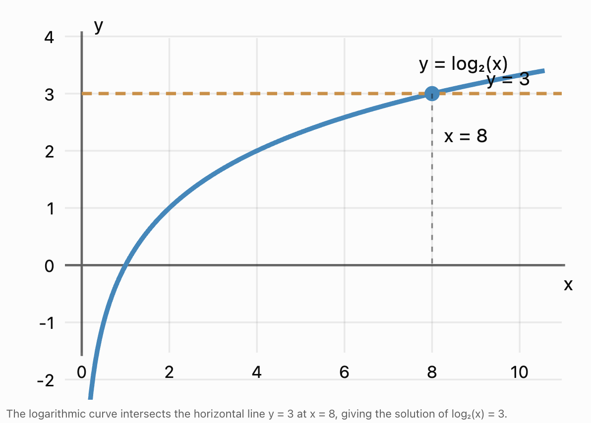
Logarithmic equations can also be solved by graphing.

Consider:

log₂(x) = 3

Graph:

y = log₂(x)

and:

y = 3

The solution is the x-coordinate of their intersection.

Advantages of Graphical Methods

Graphing can help:

• Estimate solutions.

• Identify the number of solutions.

• Detect possible extraneous solutions.

• Compare two logarithmic functions.

• Check algebraic calculations.

For more complicated equations, a graphing calculator or mathematical software may be useful.

Numerical Solutions of Logarithmic Equations

Some logarithmic equations cannot be solved using elementary algebraic methods.

For example:

ln(x) = x − 2

The variable appears both inside and outside the logarithm.

Rearrange:

f(x) = ln(x) − x + 2

A numerical method can find values where:

f(x) = 0

This equation has two real solutions:

x ≈ 0.159 and x ≈ 3.146

These can be found using graphing technology or numerical root-finding methods.

Verification

For x ≈ 0.159:

ln(0.159) ≈ −1.839

0.159 − 2 = −1.841

The values are close.

For x ≈ 3.146:

ln(3.146) ≈ 1.146

3.146 − 2 = 1.146

Both are approximate solutions.

Practical Application: pH Calculations

The pH scale measures acidity using a logarithmic relationship.

The mathematical definition is:

pH = −log₁₀(a_H⁺)

where a_H⁺ is dimensionless hydrogen-ion activity.

In dilute aqueous solutions, activity is often approximated using concentration relative to 1 mol/L.

Worked Example

A solution has pH 4.2.

Calculate its hydrogen-ion activity.

Step 1: Write the Formula

4.2 = −log₁₀(a_H⁺)

Step 2: Multiply by −1

−4.2 = log₁₀(a_H⁺)

Step 3: Convert to Exponential Form

a_H⁺ = 10⁻⁴·²

Step 4: Calculate

a_H⁺ ≈ 6.31 × 10⁻⁵

Interpretation

The hydrogen-ion activity is approximately 6.31 × 10⁻⁵.

For a sufficiently dilute solution, this corresponds approximately to a hydrogen-ion concentration of 6.31 × 10⁻⁵ mol/L.

Practical Application: Earthquake Magnitude

A simplified logarithmic relationship for earthquake magnitude is:

M = log₁₀(A/A₀)

where:

• M is magnitude.

• A is corrected seismic-wave amplitude.

• A₀ is a reference amplitude.

Actual earthquake magnitude calculations include additional measurement corrections, and modern seismology commonly uses moment magnitude.

Worked Example

An earthquake has magnitude 5.6.

Find the ratio A/A₀.

Step 1: Substitute

5.6 = log₁₀(A/A₀)

Step 2: Convert to Exponential Form

A/A₀ = 10⁵·⁶

Step 3: Calculate

A/A₀ ≈ 398107

Interpretation

The corrected amplitude is approximately 398000 times the reference amplitude in this simplified model.

Practical Application: Sound Intensity

Sound intensity level is measured using the decibel scale.

The formula is:

L = 10log₁₀(I/I₀)

where:

• L is sound intensity level in decibels.

• I is measured sound intensity.

• I₀ is reference intensity.

Worked Example

A sound has an intensity level of 70 dB.

Find its intensity relative to the reference intensity.

Step 1: Substitute

70 = 10log₁₀(I/I₀)

Step 2: Divide by 10

7 = log₁₀(I/I₀)

Step 3: Convert to Exponential Form

I/I₀ = 10⁷

Final Answer

I/I₀ = 10000000

The sound intensity is ten million times the reference intensity.

If I₀ = 10⁻¹² W/m², then:

I = 10⁷ × 10⁻¹²

I = 10⁻⁵ W/m²

Practical Application: Finding Time in Growth Models

Logarithmic equations are often used to solve for time in exponential models.

Consider:

P(t) = P₀e^(kt)

where:

• P(t) is the population at time t.

• P₀ is the initial population.

• k is the continuous growth rate.

• t is time.

Worked Example

A population grows according to:

P(t) = 2000e^(0.08t)

Find when the population reaches 5000.

Step 1: Substitute

5000 = 2000e^(0.08t)

Step 2: Divide

2.5 = e^(0.08t)

Step 3: Take Natural Logarithms

ln(2.5) = 0.08t

Step 4: Solve

t = ln(2.5)/0.08

Step 5: Calculate

t ≈ 11.45

Interpretation

The population reaches 5000 after approximately 11.45 time units.

Although the unknown appears in an exponent in the original model, logarithms make it possible to solve for time.

Practical Application: Compound Interest

The compound interest formula is:

A = P(1 + r/n)^(nt)

where:

• A is the final amount.

• P is the initial principal.

• r is the annual interest rate.

• n is the number of compounding periods per year.

• t is time in years.

Worked Example

An investment of $4000 earns 6% annual interest, compounded monthly.

How long will it take to reach $7000?

Step 1: Substitute

7000 = 4000(1 + 0.06/12)^(12t)

Step 2: Simplify

1.75 = 1.005^(12t)

Step 3: Take Natural Logarithms

ln(1.75) = 12t ln(1.005)

Step 4: Solve

t = ln(1.75)/[12ln(1.005)]

Step 5: Calculate

t ≈ 9.35 years

Interpretation

The investment reaches $7000 after approximately 9.35 years according to the continuous-time solution of the monthly-compounding formula.

Because interest is credited monthly, the balance first reaches at least $7000 after 113 complete months, or approximately 9.42 years.

A Systematic Method for Solving Logarithmic Equations

The following method works for many logarithmic equations.

Step 1: Identify the Domain

Determine the restrictions that make every logarithmic argument positive.

Step 2: Simplify the Equation

Use algebra to isolate logarithmic expressions where possible.

Step 3: Apply Logarithm Rules

Use the product, quotient, and power rules to combine or simplify logarithms.

Step 4: Convert to Exponential Form

When possible, remove the logarithm by rewriting the equation exponentially.

Step 5: Solve the Algebraic Equation

Use factoring, rearrangement, substitution, or the quadratic formula.

Step 6: Check Candidate Solutions

Reject values that violate the original domain restrictions.

Step 7: Verify in the Original Equation

Substitute each remaining candidate into the original equation.

Step 8: Interpret the Answer

For practical problems, explain the result using appropriate units and context.

Common Mistakes

Ignoring domain restrictions

Every logarithmic argument must be strictly positive.

Accepting extraneous solutions

A value obtained from algebraic manipulation is not automatically a valid logarithmic solution.

Combining logarithms incorrectly

The product rule applies to multiplication, not addition inside the argument.

Applying the quotient rule incorrectly

The difference of logarithms becomes the logarithm of a quotient.

Equating arguments with different logarithmic bases

Arguments can be equated directly only when the logarithms have the same valid base.

Forgetting the power rule

Coefficients outside logarithms can be moved into exponents.

Assuming logarithms cannot be negative

Logarithmic values may be negative even though their arguments must be positive.

Confusing logarithmic and exponential forms

Remember:

logₐ(x) = b means x = aᵇ.

Failing to verify solutions

Solutions should always be checked in the original equation.

Rounding too early

Keep exact expressions until the final calculation.

Ignoring the meaning of the result

Practical logarithmic solutions should be interpreted in context.

Key Terms

• Logarithmic Equation: An equation containing one or more logarithmic expressions involving an unknown variable.

• Logarithm: The exponent required to raise a base to a positive argument.

• Base: The positive number, other than 1, used in a logarithmic expression.

• Argument: The expression inside a logarithm.

• Domain: The set of allowable input values.

• Domain Restriction: A condition that limits the values a variable may take.

• Extraneous Solution: A candidate solution that does not satisfy the original equation.

• Verification: Checking a solution by substituting it into the original equation.

• Exponential Form: A mathematical expression involving a base raised to a power.

• Logarithmic Form: An equivalent expression identifying an exponent.

• Inverse Function: A function that reverses another function.

• Product Rule: A logarithmic property that converts multiplication into addition.

• Quotient Rule: A logarithmic property that converts division into subtraction.

• Power Rule: A logarithmic property that converts an exponent into a multiplier.

• One-to-One Function: A function in which different inputs produce different outputs.

• Natural Logarithm: A logarithm with base e.

• Common Logarithm: A logarithm with base 10.

• Change-of-Base Formula: A formula that rewrites a logarithm using a different base.

• Factorisation: Rewriting an expression as a product of factors.

• Quadratic Equation: An equation whose highest variable power is 2.

• Quadratic Formula: A formula used to solve quadratic equations.

• Substitution: Replacing an expression with a simpler variable.

• Graphical Solution: A solution identified using graphs.

• Numerical Solution: An approximate solution found through calculation.

• Approximation: A numerical value close to an exact result.

• pH: A logarithmic measure related to hydrogen-ion activity.

• Earthquake Magnitude: A measure of earthquake size determined from seismic measurements.

• Decibel: A logarithmic unit used to express ratios such as sound intensity.

• Compound Interest: Interest calculated on an initial principal and previously accumulated interest.

• Exponential Growth: Growth by a constant multiplicative factor over equal time intervals.

• Mathematical Model: A mathematical representation of a real-world system.

Key Takeaways

• Logarithmic equations contain unknown variables inside logarithmic expressions.

• The relationship between logarithmic and exponential forms is essential for solving these equations.

• Basic logarithmic equations can be solved by converting them into exponential form.

• More complicated equations may require logarithmic properties and algebraic manipulation.

• The product rule combines sums of logarithms into the logarithm of a product.

• The quotient rule combines differences of logarithms into the logarithm of a quotient.

• The power rule converts coefficients into exponents.

• Logarithms with the same valid base can have their arguments equated when both arguments are positive.

• Every logarithmic argument in the original equation must be strictly positive.

• Domain restrictions should be identified before solving.

• Algebraic manipulation can introduce extraneous solutions.

• Candidate solutions must be checked against the original domain restrictions.

• Substitution can simplify equations containing repeated logarithmic expressions.

• Quadratic equations may arise when logarithms are combined.

• Graphical methods help estimate solutions and determine how many solutions exist.

• Numerical methods are useful when elementary algebraic solutions are unavailable.

• Natural logarithms are particularly useful for models involving e.

• Logarithmic equations are used in chemistry, geology, acoustics, finance, and population modelling.

• Verification ensures that proposed solutions satisfy the original equation.

• A complete logarithmic solution requires correct algebra, careful domain analysis, and verification of every candidate answer.

Check Your Understanding

Recall and Understanding

1. Explain what makes an equation a logarithmic equation.

2. Describe why logarithmic arguments must be positive.

3. Define an extraneous solution and explain how one can arise.

4. Explain when two logarithmic arguments can be equated directly.

5. Describe the difference between solving a logarithmic equation algebraically and graphically.

Application

6. Solve log₂(x) = 7.

7. Solve log₃(2x − 5) = 3.

8. Solve log₄(x + 3) = log₄(2x − 1).

9. Solve log₂(x) + log₂(x − 4) = 5, checking for extraneous solutions.

10. Solve ln(3x + 2) = 4, giving your answer to three decimal places.

Analysis and Challenge

11. Solve log₃(x + 4) − log₃(x − 2) = 2, stating the domain.

12. Solve [log₂(x)]² − 5log₂(x) + 6 = 0.

13. Solve log₂(x) + log₂(x − 1) − log₂(x + 3) = 1, checking all candidate solutions.

14. A solution has pH 3.6. Calculate its hydrogen-ion activity and explain the result.

15. An investment grows according to A = 6000(1.045)ᵗ. Determine when it reaches $10000 and explain how logarithms are used in the solution.

Final Summary

Logarithmic equations can be solved by converting logarithmic expressions into exponential form and applying appropriate algebraic techniques.

The properties of logarithms allow equations containing multiple logarithmic terms to be simplified and combined.

More advanced equations may require factoring, the quadratic formula, substitution, graphical methods, or numerical approximations.

A particularly important feature of logarithmic equations is the possibility of extraneous solutions.

Because logarithmic arguments must be positive, every candidate solution must satisfy the original domain restrictions.

Verification is essential to ensure that a calculated answer is mathematically valid.

Logarithmic equations also have important real-world applications, including pH calculations, earthquake magnitude comparisons, sound intensity measurements, compound interest, and exponential growth models.

The central principle is that solving logarithmic equations requires more than finding an algebraic answer: every solution must satisfy the original logarithmic equation and its domain restrictions.