Exponential and Logarithmic Equations
| Site: | Young Education |
| Cursus: | Exponential and Logarithmic Functions |
| Boek: | Exponential and Logarithmic Equations |
| Afgedrukt door: | Guest user |
| Datum: | maandag, 9 november 2026, 16:40 |
1. Solving Exponential Equations
Learning outcomes
- I can solve exponential equations with common bases.
- I can solve exponential equations using logarithms.
- I can verify exponential solutions.
- I can solve equations with multiple exponential terms.
- I can apply exponential equations to practical problems.
Solving Exponential Equations
Introduction to Exponential Equations
Exponential equations are equations in which the unknown variable appears in an exponent.
For example:
2ˣ = 32
Unlike ordinary algebraic equations, where the variable is usually multiplied, divided, added, or subtracted, exponential equations involve a variable controlling a power.
Exponential equations are important because many real-world processes involve repeated multiplication rather than constant addition.
Examples include:
-
Population growth.
-
Compound interest.
-
Radioactive decay.
-
Bacterial reproduction.
-
Depreciation of assets.
-
Medication elimination.
-
Cooling and heating processes.
-
Growth of digital information.
There are several methods for solving exponential equations. The most appropriate method depends on the structure of the equation.
The main approaches are:
-
Expressing both sides using a common base.
-
Using logarithms to isolate an unknown exponent.
-
Applying substitution to equations with multiple exponential terms.
-
Factoring exponential expressions.
-
Using numerical or graphical methods when algebraic solutions are difficult.


Understanding Exponential Equations
An exponential equation contains a variable in an exponent.
Examples include:
3ˣ = 81
5^(2x) = 125
2ˣ = 15
4ˣ + 2ˣ = 20
e^(0.5x) = 12
These equations may look different, but they all involve exponential relationships.
Exponential Equations Versus Power Equations
Consider:
x³ = 27
This is a power equation because the variable is the base.
Now consider:
3ˣ = 27
This is an exponential equation because the variable is the exponent.
The distinction matters because the equations are solved differently.
For x³ = 27, we take a cube root.
For 3ˣ = 27, we identify the exponent that produces 27.
Reviewing the Laws of Exponents
The laws of exponents are essential when solving exponential equations.
|
Exponent law |
General rule |
Example |
|---|---|---|
|
Product |
aᵐ × aⁿ = a^(m+n) |
2³ × 2² = 2⁵ |
|
Quotient |
aᵐ/aⁿ = a^(m−n) |
3⁵/3² = 3³ |
|
Power of a power |
(aᵐ)ⁿ = a^(mn) |
(2³)² = 2⁶ |
|
Zero exponent |
a⁰ = 1 |
5⁰ = 1 |
|
Negative exponent |
a⁻ⁿ = 1/aⁿ |
2⁻³ = 1/8 |
|
Fractional exponent |
a^(1/n) = ⁿ√a |
16^(1/2) = 4 |
For the methods in this lesson, exponential bases are generally assumed to be positive.
Solving Exponential Equations Using Common Bases
The simplest exponential equations can be solved by expressing both sides using the same base.
The fundamental property is:
If aᵐ = aⁿ, then m = n, provided a > 0 and a ≠ 1.
This works because an exponential function with a valid base is one-to-one.
Worked Example: Basic Common Bases
Solve:
2ˣ = 64
Step 1: Rewrite 64 as a Power of 2
64 = 2⁶
Therefore:
2ˣ = 2⁶
Step 2: Equate Exponents
x = 6
Step 3: Verify
2⁶ = 64
Final Answer: x = 6
Common Bases with Algebraic Exponents
Worked Example
Solve:
3^(2x−1) = 81
Step 1: Rewrite Using a Common Base
81 = 3⁴
Therefore:
3^(2x−1) = 3⁴
Step 2: Equate Exponents
2x − 1 = 4
Step 3: Solve
2x = 5
x = 5/2 = 2.5
Step 4: Verify
3^[2(2.5)−1] = 3⁴ = 81
The solution is correct.
Rewriting Different Bases
Sometimes the two sides initially have different bases, but both can be expressed using powers of a common number.
Worked Example
Solve:
4ˣ = 8^(x−1)
Step 1: Rewrite Both Sides Using Base 2
4 = 2²
8 = 2³
Therefore:
(2²)ˣ = (2³)^(x−1)
Step 2: Apply the Power-of-a-Power Rule
2^(2x) = 2^(3x−3)
Step 3: Equate Exponents
2x = 3x − 3
Step 4: Solve
x = 3
Step 5: Verify
Left side:
4³ = 64
Right side:
8^(3−1) = 8² = 64
Both sides are equal.
Solving Equations with Fractional Bases
Fractional bases can often be rewritten using negative exponents.
Worked Example
Solve:
(1/2)ˣ = 16
Step 1: Rewrite Using Base 2
1/2 = 2⁻¹
16 = 2⁴
Therefore:
(2⁻¹)ˣ = 2⁴
Step 2: Simplify
2⁻ˣ = 2⁴
Step 3: Equate Exponents
−x = 4
x = −4
Verification
(1/2)⁻⁴ = 2⁴ = 16
The solution is correct.
Important Principle
Exponential equations can have negative solutions.
A negative exponent represents a reciprocal, not a negative output.
Solving Equations with Fractional Exponents
Worked Example
Solve:
9^(x/2) = 27
Step 1: Rewrite Using Base 3
9 = 3²
27 = 3³
Therefore:
(3²)^(x/2) = 3³
Step 2: Simplify
3ˣ = 3³
Step 3: Equate Exponents
x = 3
Verification
9^(3/2) = (√9)³ = 3³ = 27
The solution is correct.
Solving Exponential Equations Using Logarithms
Not all exponential equations can be rewritten using convenient common bases.
Consider:
2ˣ = 13
The number 13 is not an integer power of 2.
We know:
2³ = 8
2⁴ = 16
Therefore, the solution lies between 3 and 4.
To find a more accurate answer, we use logarithms.
The Connection Between Exponents and Logarithms
Recall:
aˣ = b ⇔ x = logₐ(b)
Using the change-of-base formula:
x = ln(b)/ln(a)
or:
x = log(b)/log(a)
This allows us to solve exponential equations even when the answer is not a simple integer or fraction.
Worked Example: Using Logarithms
Solve:
2ˣ = 13
Step 1: Take Natural Logarithms
ln(2ˣ) = ln(13)
Step 2: Apply the Power Rule
x ln(2) = ln(13)
Step 3: Isolate x
x = ln(13)/ln(2)
Step 4: Calculate
x ≈ 3.700
Step 5: Verify
2³·⁷ ≈ 12.996
This is approximately 13.
The small difference is caused by rounding.
The exact solution remains:
x = ln(13)/ln(2)
Solving Equations with More Complicated Exponents
Worked Example
Solve:
5^(3x−2) = 40
Step 1: Take Natural Logarithms
ln[5^(3x−2)] = ln(40)
Step 2: Apply the Power Rule
(3x − 2)ln(5) = ln(40)
Step 3: Divide by ln(5)
3x − 2 = ln(40)/ln(5)
Step 4: Isolate x
3x = 2 + ln(40)/ln(5)
x = [2 + ln(40)/ln(5)]/3
Step 5: Calculate
x ≈ 1.431
Verification
Substitute the unrounded solution into the original equation:
5^(3x−2) = 40
The equation is satisfied.
Solving Equations Involving e
The number e is an important mathematical constant:
e ≈ 2.71828
Exponential equations involving e are especially common in calculus and scientific modelling.
The natural logarithm, ln, is the inverse of the exponential function with base e.
Therefore:
ln(eˣ) = x
Worked Example
Solve:
e^(2x) = 15
Step 1: Take Natural Logarithms
ln(e^(2x)) = ln(15)
Step 2: Simplify
2x = ln(15)
Step 3: Solve
x = ln(15)/2
x ≈ 1.354
Verification
e^[2(1.354)] ≈ 15
The answer is reasonable.
Exponential Equations with Coefficients
Sometimes an exponential term is multiplied by a constant.
Worked Example
Solve:
4 × 3ˣ = 100
Step 1: Isolate the Exponential Term
3ˣ = 25
Step 2: Take Logarithms
ln(3ˣ) = ln(25)
Step 3: Apply the Power Rule
x ln(3) = ln(25)
Step 4: Solve
x = ln(25)/ln(3)
x ≈ 2.930
Important Strategy
Always simplify the equation and isolate the exponential expression before applying logarithms.
Exponential Equations with Terms on Both Sides
Worked Example
Solve:
2^(x+1) = 5^(x−2)
The bases cannot be rewritten conveniently using a common base.
Step 1: Take Natural Logarithms
ln[2^(x+1)] = ln[5^(x−2)]
Step 2: Apply the Power Rule
(x + 1)ln(2) = (x − 2)ln(5)
Step 3: Expand
x ln(2) + ln(2) = x ln(5) − 2ln(5)
Step 4: Collect Terms
x ln(2) − x ln(5) = −2ln(5) − ln(2)
Factorise:
x[ln(2) − ln(5)] = −2ln(5) − ln(2)
Step 5: Solve
x = [2ln(5) + ln(2)]/[ln(5) − ln(2)]
Step 6: Calculate
x ≈ 4.269
This demonstrates how logarithms transform an exponential equation into a linear equation.
Solving Equations with Multiple Exponential Terms
Some exponential equations contain several terms involving the unknown exponent.
For example:
2^(2x) − 5(2ˣ) + 4 = 0
These equations can often be solved using substitution.
The key idea is to recognise that:
2^(2x) = (2ˣ)²
This produces a quadratic structure.
Substitution Method
Worked Example
Solve:
2^(2x) − 5(2ˣ) + 4 = 0
Step 1: Identify the Repeated Exponential Expression
Let:
u = 2ˣ
Then:
2^(2x) = u²
Step 2: Rewrite the Equation
u² − 5u + 4 = 0
Step 3: Factorise
(u − 1)(u − 4) = 0
Therefore:
u = 1
or:
u = 4
Step 4: Substitute Back
Since u = 2ˣ:
Case 1
2ˣ = 1
2ˣ = 2⁰
x = 0
Case 2
2ˣ = 4
2ˣ = 2²
x = 2
Final Answer
x = 0 or x = 2
Verification
For x = 0:
2⁰ − 5(1) + 4 = 0
For x = 2:
2⁴ − 5(4) + 4 = 16 − 20 + 4 = 0
Both solutions are valid.
Substitution with Other Bases
Worked Example
Solve:
3^(2x) − 10(3ˣ) + 9 = 0
Step 1: Substitute
Let:
u = 3ˣ
Then:
u² − 10u + 9 = 0
Step 2: Factorise
(u − 1)(u − 9) = 0
Therefore:
u = 1 or u = 9
Step 3: Substitute Back
3ˣ = 1
x = 0
or:
3ˣ = 9
x = 2
Final Answer
x = 0 or x = 2
Substitution with a Quadratic Formula
Not every transformed equation factorises easily.
Worked Example
Solve:
4ˣ − 3(2ˣ) − 2 = 0
Step 1: Rewrite
Since:
4ˣ = (2ˣ)²
the equation becomes:
(2ˣ)² − 3(2ˣ) − 2 = 0
Step 2: Substitute
Let:
u = 2ˣ
Then:
u² − 3u − 2 = 0
Step 3: Apply the Quadratic Formula
u = [3 ± √(9 + 8)]/2
u = [3 ± √17]/2
Step 4: Check the Possible Values
Since:
u = 2ˣ > 0
only positive values of u are valid.
The two quadratic roots are:
u = (3 + √17)/2 ≈ 3.562
u = (3 − √17)/2 ≈ −0.562
Reject the negative root.
Step 5: Solve the Exponential Equation
2ˣ = (3 + √17)/2
Take logarithms:
x = ln[(3 + √17)/2]/ln(2)
x ≈ 1.832
Important Principle
When substituting u = aˣ, remember that u must be positive.
A negative quadratic solution cannot represent a positive-base exponential expression.
Factoring Exponential Expressions
Some exponential equations can be simplified by factoring.
Worked Example
Solve:
3^(x+1) + 3ˣ = 108
Step 1: Rewrite the First Term
3^(x+1) = 3 × 3ˣ
Therefore:
3(3ˣ) + 3ˣ = 108
Step 2: Factor
4(3ˣ) = 108
Step 3: Divide
3ˣ = 27
Step 4: Solve
3ˣ = 3³
x = 3
Verification
3⁴ + 3³ = 81 + 27 = 108
The solution is correct.
Equations with Three or More Exponential Terms
Worked Example
Solve:
2^(x+2) − 2^(x+1) − 2ˣ = 16
Step 1: Rewrite Every Term
2^(x+2) = 4 × 2ˣ
2^(x+1) = 2 × 2ˣ
Therefore:
4(2ˣ) − 2(2ˣ) − 2ˣ = 16
Step 2: Combine Like Terms
(4 − 2 − 1)2ˣ = 16
2ˣ = 16
Step 3: Solve
2ˣ = 2⁴
x = 4
Verification
2⁶ − 2⁵ − 2⁴ = 64 − 32 − 16 = 16
The solution is correct.
Graphical Solutions of Exponential Equations
Exponential equations can also be solved graphically.
Consider:
2ˣ = 10
Graph:
y = 2ˣ
and:
y = 10
The solution is the x-coordinate of their intersection.
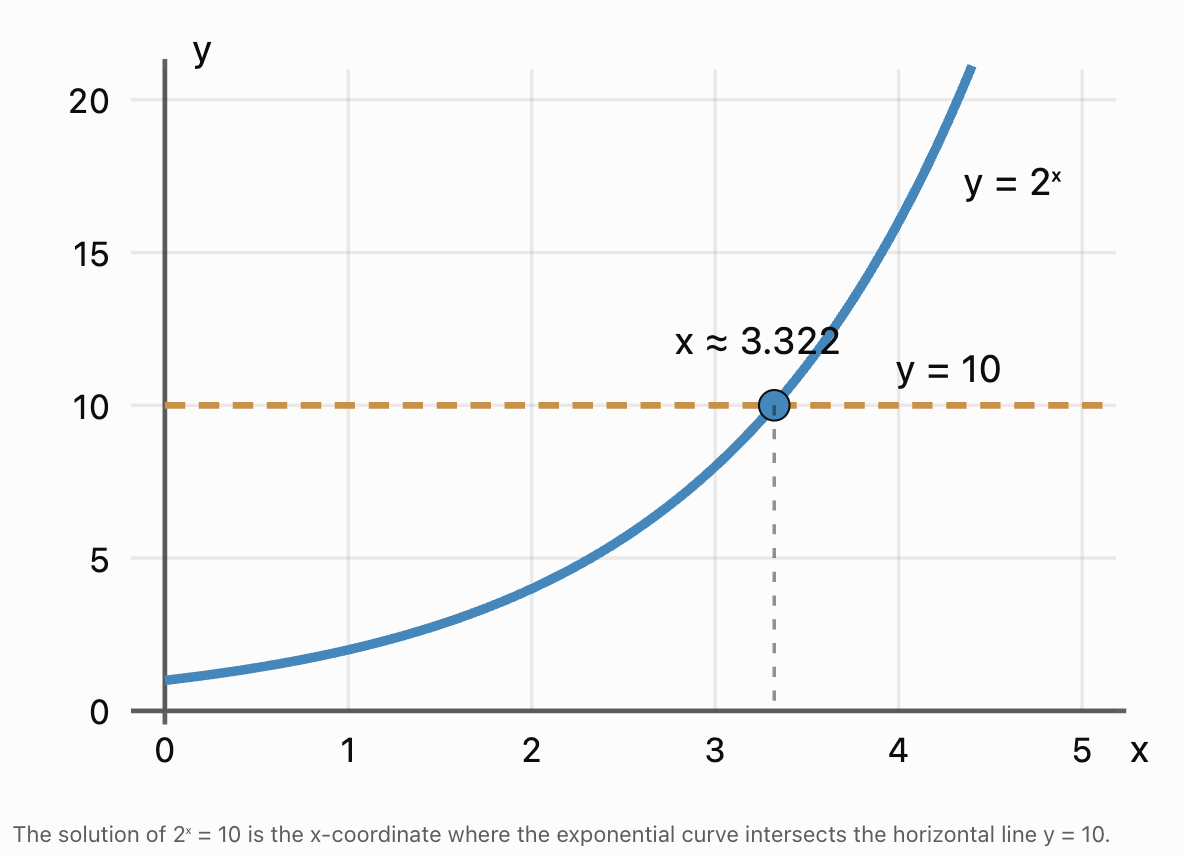
The graph gives:
x ≈ 3.322
This agrees with the logarithmic solution:
x = ln(10)/ln(2)
Advantages of Graphical Methods
Graphs can help:
-
Estimate solutions.
-
Identify whether solutions exist.
-
Determine the number of solutions.
-
Check algebraic answers.
-
Solve equations that are difficult to rearrange.
However, graphical answers may be approximate.
Numerical Methods
Some exponential equations cannot be solved using simple algebraic methods.
For example:
2ˣ = x + 3
The variable appears both in an exponent and outside it.
This equation has two real solutions.
Numerical methods can approximate them by finding the zeros of:
f(x) = 2ˣ − x − 3
Using graphing or numerical root-finding technology gives approximately:
x ≈ −2.863 and x ≈ 2.445
Numerical methods are useful when exact algebraic solutions are unavailable or impractical.
Practical Application: Compound Interest
Exponential equations are frequently used in finance.
For compound interest:
A = P(1 + r/n)^(nt)
where:
-
A = final amount.
-
P = initial principal.
-
r = annual interest rate as a decimal.
-
n = number of compounding periods per year.
-
t = time in years.
Worked Example: Doubling an Investment
An investment earns 5% interest annually, compounded once per year.
How long will it take to double?
Step 1: Write the Equation
A = P(1.05)ᵗ
For doubling:
2P = P(1.05)ᵗ
Step 2: Simplify
2 = 1.05ᵗ
Step 3: Take Logarithms
ln(2) = t ln(1.05)
Step 4: Solve
t = ln(2)/ln(1.05)
t ≈ 14.21 years
Interpretation
The investment doubles after approximately 14.21 years according to the exponential model.
With interest credited only at the end of each year, the account first reaches at least twice its original value after 15 complete years.

Practical Application: Population Growth
Suppose a population grows by 6% each year.
The population is modelled by:
P(t) = P₀(1.06)ᵗ
Worked Example
A town has an initial population of 12000.
How long will it take to reach 20000?
Step 1: Substitute
20000 = 12000(1.06)ᵗ
Step 2: Divide
20000/12000 = 1.06ᵗ
5/3 = 1.06ᵗ
Step 3: Take Logarithms
ln(5/3) = t ln(1.06)
Step 4: Solve
t = ln(5/3)/ln(1.06)
t ≈ 8.77 years
Interpretation
The population reaches 20000 after approximately 8.77 years under the model.
This assumes the annual proportional growth rate remains constant.
Practical Application: Radioactive Decay
Radioactive substances decay exponentially.
A common model is:
N(t) = N₀e^(−λt)
where:
-
N(t) = amount remaining after time t.
-
N₀ = initial amount.
-
λ = decay constant.
-
t = elapsed time.
Worked Example
A radioactive substance has a decay constant of 0.04 per year.
How long will it take for 25% of the original material to remain?
Step 1: Write the Equation
0.25N₀ = N₀e^(−0.04t)
Step 2: Divide
0.25 = e^(−0.04t)
Step 3: Take Natural Logarithms
ln(0.25) = −0.04t
Step 4: Solve
t = ln(0.25)/(−0.04)
t ≈ 34.66 years
Interpretation
Approximately 34.66 years are required for the substance to decrease to 25% of its original amount.
Practical Application: Bacterial Growth
Bacteria may reproduce through binary fission, causing populations to increase exponentially under suitable conditions.
Suppose a bacterial population doubles every 3 hours.
The model is:
N(t) = N₀ × 2^(t/3)
Worked Example
A bacterial population begins with 500 bacteria.
How long will it take to reach 8000 bacteria?
Step 1: Substitute
8000 = 500 × 2^(t/3)
Step 2: Divide
16 = 2^(t/3)
Step 3: Rewrite Using a Common Base
16 = 2⁴
Therefore:
2⁴ = 2^(t/3)
Step 4: Equate Exponents
4 = t/3
t = 12 hours
Interpretation
The population doubles four times:
500 → 1000 → 2000 → 4000 → 8000
Four doubling periods of 3 hours each give 12 hours.
Practical Application: Depreciation
Depreciation describes the decrease in the value of an asset over time.
A simplified depreciation model is:
V(t) = V₀(1 − r)ᵗ
where:
-
V(t) = value after t years.
-
V₀ = initial value.
-
r = annual depreciation rate.
Worked Example
A vehicle costs $30000 and loses 15% of its value each year.
When will its value fall to $10000?
Step 1: Write the Equation
10000 = 30000(0.85)ᵗ
Step 2: Divide
1/3 = 0.85ᵗ
Step 3: Take Logarithms
ln(1/3) = t ln(0.85)
Step 4: Solve
t = ln(1/3)/ln(0.85)
t ≈ 6.76 years
Interpretation
The vehicle's value falls to $10000 after approximately 6.76 years under the constant-rate depreciation model.
Practical Application: Medication Elimination
Some medications are eliminated from the body approximately exponentially over certain concentration ranges.
A simplified model is:
C(t) = C₀e^(−kt)
where:
-
C(t) = concentration at time t.
-
C₀ = initial concentration.
-
k = elimination constant.
Worked Example
A medication concentration decreases according to:
C(t) = 80e^(−0.2t)
where t is measured in hours.
When will the concentration reach 20 units?
Step 1: Substitute
20 = 80e^(−0.2t)
Step 2: Divide
0.25 = e^(−0.2t)
Step 3: Take Natural Logarithms
ln(0.25) = −0.2t
Step 4: Solve
t = ln(0.25)/(−0.2)
t ≈ 6.93 hours
This is a mathematical model; actual medication elimination can depend on multiple biological processes.
Verifying Exponential Solutions
Verification is an important part of solving exponential equations.
A solution should satisfy the original equation, not merely a transformed version.
Verification Method
-
Substitute the calculated value into the original equation.
-
Evaluate the left-hand side.
-
Evaluate the right-hand side.
-
Compare the results.
-
Account for rounding if the solution is approximate.
Worked Example
Verify:
x = 2
for:
3^(x+1) = 27
Substitute:
3^(2+1) = 3³ = 27
The left side equals the right side.
Therefore:
x = 2 is valid.
Verifying Approximate Solutions
Suppose:
2ˣ = 13
and:
x ≈ 3.700
Substitution gives:
2³·⁷⁰⁰ ≈ 12.996
This is close to 13.
The slight difference is due to rounding.
For greater accuracy, use the unrounded logarithmic expression.
Checking for Extraneous or Invalid Solutions
When solving exponential equations by substitution, not every algebraic solution is necessarily valid.
For example:
2^(2x) + 2ˣ − 6 = 0
Let:
u = 2ˣ
Then:
u² + u − 6 = 0
Factorise:
(u + 3)(u − 2) = 0
Therefore:
u = −3 or u = 2
However:
2ˣ > 0
for every real x.
Thus:
u = −3 is impossible.
Only:
2ˣ = 2
is valid.
Therefore:
x = 1
The positivity of exponential expressions is an important restriction.
Choosing the Best Solution Method
|
Equation type |
Recommended method |
|---|---|
|
2ˣ = 32 |
Common bases |
|
3^(2x) = 81 |
Common bases |
|
4ˣ = 8^(x−1) |
Rewrite using a common base |
|
2ˣ = 13 |
Logarithms |
|
5^(3x−2) = 40 |
Logarithms and algebra |
|
e^(2x) = 15 |
Natural logarithms |
|
2^(2x) − 5(2ˣ) + 4 = 0 |
Substitution |
|
3^(x+1) + 3ˣ = 108 |
Factoring |
|
2ˣ = x + 3 |
Numerical or graphical methods |
The goal is not simply to memorise methods, but to recognise the structure of the equation and select an efficient strategy.
Common Mistakes
Confusing exponential equations with power equations
The variable's position determines the appropriate solution method.
Equating exponents when the bases are different
Exponents can be equated directly only when both sides have the same valid base.
Applying logarithms incorrectly
Logarithms must be applied to both sides of an equation, and their arguments must be positive.
Forgetting the logarithmic power rule
For example:
ln(3ˣ) = xln(3)
not ln(3x).
Taking logarithms of individual terms in a sum
In general:
ln(a + b) ≠ ln(a) + ln(b)
Forgetting to isolate the exponential expression
Simplify coefficients and constants before taking logarithms where possible.
Incorrectly rewriting exponential expressions
Remember:
a^(x+1) = a × aˣ
and:
a^(2x) = (aˣ)²
Ignoring the positivity of exponential expressions
If u = aˣ with a > 0, then u must be positive.
Keeping invalid solutions after substitution
Solutions to the transformed quadratic must satisfy the original exponential equation.
Rounding intermediate calculations too early
Keep exact logarithmic expressions until the final step.
Failing to verify solutions
Substitution into the original equation helps detect errors.
Ignoring practical limitations
Exponential models assume particular growth or decay patterns that may not continue indefinitely.
Key Terms
-
Exponential Equation: An equation in which the unknown variable appears in an exponent.
-
Base: The number raised to a power.
-
Exponent: The power to which a base is raised.
-
Exponential Function: A function in which the variable appears in an exponent.
-
Common Base: A shared base used to rewrite both sides of an exponential equation.
-
One-to-One Function: A function in which distinct inputs produce distinct outputs.
-
Logarithm: The exponent required to produce a given positive number from a fixed base.
-
Natural Logarithm: A logarithm with base e.
-
Common Logarithm: A logarithm with base 10.
-
Inverse Function: A function that reverses another function.
-
Change-of-Base Formula: A formula used to rewrite logarithms using a different base.
-
Power Rule of Logarithms: A rule allowing an exponent to become a multiplier outside a logarithm.
-
Exponent Laws: Mathematical rules describing operations involving powers.
-
Substitution: Replacing a complicated expression with a simpler variable.
-
Quadratic Equation: An equation containing a squared variable as its highest power.
-
Factorisation: Rewriting an expression as a product of factors.
-
Quadratic Formula: A formula used to solve quadratic equations.
-
Graphical Solution: A solution found by examining intersections or zeros on a graph.
-
Numerical Method: A procedure for approximating solutions using calculations.
-
Verification: Checking a solution by substituting it into the original equation.
-
Extraneous Solution: A candidate solution produced during manipulation that does not satisfy the original equation.
-
Exponential Growth: Growth by a constant multiplicative factor over equal time intervals.
-
Exponential Decay: Decrease by a constant multiplicative factor over equal time intervals.
-
Growth Rate: The rate at which a quantity increases.
-
Decay Constant: A parameter describing continuous exponential decay.
-
Doubling Time: The time required for a growing quantity to become twice its initial value.
-
Half-Life: The time required for a decaying quantity to decrease to half its original value.
-
Compound Interest: Interest calculated on an initial principal and previously accumulated interest.
-
Depreciation: A decrease in an asset's value over time.
-
Mathematical Model: A mathematical representation of a real-world system.
-
Approximate Solution: A numerical value close to an exact solution.
-
Exact Solution: A solution expressed without numerical rounding.
Key Takeaways
-
Exponential equations contain variables in exponents.
-
Exponential equations can often be solved by rewriting both sides using a common base.
-
When the bases are equal and valid, their exponents can be equated.
-
Exponent laws help simplify exponential expressions before solving.
-
Fractional and negative exponents can be rewritten using familiar bases.
-
Logarithms allow exponential equations to be solved when common bases are unavailable.
-
The natural logarithm is especially useful for equations involving e.
-
The logarithmic power rule transforms an exponential equation into an algebraic equation.
-
Exponential equations with multiple terms may be simplified by factoring.
-
Substitution can transform some exponential equations into quadratic equations.
-
When substituting u = aˣ, only positive values of u are valid.
-
Some exponential equations require numerical or graphical methods.
-
Graphs help identify the number and approximate locations of solutions.
-
Verification is essential, particularly after substitution or algebraic manipulation.
-
Exact logarithmic expressions should be retained until the final calculation.
-
Exponential equations are widely used in finance, population biology, radioactive decay, and other scientific models.
-
Growth models involve increasing exponential functions, while decay models involve decreasing exponential functions.
-
Practical solutions must be interpreted using appropriate units and assumptions.
-
Selecting the correct method depends on recognising the mathematical structure of the equation.
-
Mastering exponential equations provides an essential foundation for logarithmic equations, exponential modelling, and advanced mathematical problem solving.
Check Your Understanding
Recall and Understanding
-
Define an exponential equation and explain how it differs from a power equation.
-
Explain when exponents can be equated directly.
-
Describe why logarithms are useful for solving exponential equations.
-
Explain how substitution can transform an exponential equation into a quadratic equation.
-
Explain why the substitution u = 3ˣ requires u > 0.
Application
-
Solve 2^(3x−1) = 64.
-
Solve 9ˣ = 27^(x−1).
-
Solve 4ˣ = 30, giving your answer to three decimal places.
-
Solve e^(0.5x) = 18.
-
Solve 2^(2x) − 6(2ˣ) + 8 = 0.
Analysis and Challenge
-
Solve 3^(2x) − 12(3ˣ) + 27 = 0, checking all solutions.
-
Solve 5^(x+1) − 5ˣ = 100 using factorisation.
-
Solve 2^(x+2) = 7^(x−1), giving your answer to three decimal places.
-
A bacterial population starts at 800 and doubles every 4 hours. Determine when the population will reach 20000.
-
An investment of $10000 earns 4.5% annual interest, compounded monthly. Determine how long it takes to reach $15000, and identify the first complete month when the balance reaches or exceeds that amount.
Final Summary
Exponential equations are used to determine unknown exponents and model processes involving repeated multiplication.
When both sides of an equation can be expressed using a common base, the exponents can be equated and solved algebraically.
When common bases are unavailable, logarithms provide a powerful alternative.
More complicated equations involving multiple exponential terms can often be simplified using factoring or substitution.
Graphical and numerical methods provide additional techniques when exact algebraic solutions are difficult to obtain.
Exponential equations are particularly important in real-world situations involving population growth, compound interest, radioactive decay, depreciation, and other changing quantities.
A complete solution should use an appropriate method, preserve mathematical accuracy, verify the result, and interpret the answer in context.
The central principle is that exponential equations become manageable when we recognise their structure and use common bases, logarithms, factoring, or substitution to isolate the unknown exponent.
2. Solving Logarithmic Equations
Learning outcomes
- I can solve logarithmic equations.
- I can identify extraneous solutions.
- I can verify logarithmic solutions.
- I can solve equations involving multiple logarithms.
- I can apply logarithmic equations in context.
Solving Logarithmic Equations
Introduction to Logarithmic Equations
Logarithmic equations are equations in which the unknown variable appears inside one or more logarithms.
For example:
log₂(x) = 5
This equation asks:
"To what power must 2 be raised to produce x?"
Since:
2⁵ = 32
the solution is:
x = 32
However, logarithmic equations can become more complicated when they contain several logarithms, algebraic expressions, or logarithms on both sides.
For example:
log₃(x + 2) + log₃(x − 2) = 2
Solving these equations requires an understanding of logarithmic properties, algebraic manipulation, and domain restrictions.
One particularly important skill is identifying extraneous solutions—values that appear to solve a transformed equation but are not valid in the original logarithmic equation.
Logarithmic equations are also used in chemistry, physics, finance, biology, and other fields involving exponential relationships.


Reviewing the Meaning of Logarithms
A logarithm is the inverse of an exponential expression.
The fundamental relationship is:
logₐ(b) = c ⇔ aᶜ = b
where:
-
a is the base.
-
b is the argument.
-
c is the exponent.
For real logarithms:
-
a > 0.
-
a ≠ 1.
-
b > 0.
Example
Consider:
log₃(81) = 4
This means:
3⁴ = 81
The logarithmic and exponential statements express the same relationship.
This equivalence is the foundation for solving logarithmic equations.
The Domain of a Logarithm
Before solving a logarithmic equation, it is important to determine which values of the variable are allowed.
For:
logₐ(x)
the argument must be positive.
Therefore:
x > 0
For a more complicated logarithm:
log₂(x − 5)
the argument must satisfy:
x − 5 > 0
Therefore:
x > 5
Why This Matters
Consider:
log₂(−4)
This expression is undefined in the real number system.
No real exponent of 2 produces a negative result.
Therefore, any proposed solution that makes a logarithmic argument zero or negative must be rejected.
Important Principle
Every logarithmic argument in the original equation must be strictly positive.
This requirement is essential when checking solutions.
Solving Basic Logarithmic Equations
The simplest logarithmic equations contain one logarithm equal to a constant.
General Method
For:
logₐ(x) = b
convert to exponential form:
x = aᵇ
Worked Example
Solve:
log₂(x) = 6
Step 1: Convert to Exponential Form
x = 2⁶
Step 2: Evaluate
x = 64
Step 3: Verify
log₂(64) = 6
Since:
2⁶ = 64
the solution is correct.
Solving Logarithms with Algebraic Arguments
Worked Example
Solve:
log₃(x + 4) = 2
Step 1: Identify the Domain
x + 4 > 0
x > −4
Step 2: Convert to Exponential Form
x + 4 = 3²
Step 3: Simplify
x + 4 = 9
x = 5
Step 4: Verify
log₃(5 + 4) = log₃(9) = 2
The solution is valid.
Solving Equations with Coefficients
Sometimes a logarithm is multiplied by a constant.
Worked Example
Solve:
3log₂(x) = 12
Step 1: Divide by 3
log₂(x) = 4
Step 2: Convert to Exponential Form
x = 2⁴
x = 16
Step 3: Verify
3log₂(16) = 3(4) = 12
The equation is satisfied.
Solving Equations with Constants Outside the Logarithm
Worked Example
Solve:
2log₅(x − 1) + 3 = 7
Step 1: Identify the Domain
x − 1 > 0
x > 1
Step 2: Subtract 3
2log₅(x − 1) = 4
Step 3: Divide by 2
log₅(x − 1) = 2
Step 4: Convert to Exponential Form
x − 1 = 5²
x − 1 = 25
x = 26
Step 5: Verify
2log₅(25) + 3 = 2(2) + 3 = 7
The solution is valid.
Solving Equations with Logarithms on Both Sides
When two logarithms have the same base, their arguments can be equated, provided both arguments are positive.
The principle is:
If logₐ(M) = logₐ(N), then M = N
for valid logarithmic arguments.
This works because logarithmic functions are one-to-one.
Worked Example
Solve:
log₃(2x + 1) = log₃(x + 7)
Step 1: Identify Domain Restrictions
2x + 1 > 0
x > −1/2
Also:
x + 7 > 0
x > −7
Both conditions must hold.
Therefore:
x > −1/2
Step 2: Equate Arguments
2x + 1 = x + 7
Step 3: Solve
x = 6
Step 4: Verify
Left side:
log₃(13)
Right side:
log₃(13)
Both sides are equal, and both arguments are positive.
Therefore:
x = 6
Solving Equations with Different Bases
Logarithms with different bases cannot have their arguments equated directly.
For example:
log₂(x) = log₄(x + 2)
We must first rewrite them using a common base.
Worked Example
Solve:
log₂(x) = log₄(x + 2)
Step 1: Identify the Domain
x > 0
x + 2 > 0
Combined restriction:
x > 0
Step 2: Change Base
Since:
log₄(x + 2) = log₂(x + 2)/log₂(4)
and:
log₂(4) = 2
we obtain:
log₂(x) = (1/2)log₂(x + 2)
Step 3: Multiply by 2
2log₂(x) = log₂(x + 2)
Step 4: Apply the Power Rule
log₂(x²) = log₂(x + 2)
Step 5: Equate Arguments
x² = x + 2
Step 6: Rearrange
x² − x − 2 = 0
Factorise:
(x − 2)(x + 1) = 0
Therefore:
x = 2 or x = −1
Step 7: Check the Domain
The original equation requires x > 0.
Therefore, x = −1 is invalid.
Final Answer
x = 2
Verification
Left side:
log₂(2) = 1
Right side:
log₄(4) = 1
The solution is correct.
Solving Equations with Multiple Logarithms
Many logarithmic equations contain sums or differences of logarithms.
These equations can often be simplified using the logarithm rules.
Product Rule
logₐ(M) + logₐ(N) = logₐ(MN)
Quotient Rule
logₐ(M) − logₐ(N) = logₐ(M/N)
Power Rule
klogₐ(M) = logₐ(Mᵏ)
These rules are valid under their usual domain restrictions.
Applying the Product Rule
Worked Example
Solve:
log₂(x) + log₂(x − 2) = 3
Step 1: Identify Domain Restrictions
x > 0
x − 2 > 0
Therefore:
x > 2
Step 2: Combine the Logarithms
Using the product rule:
log₂[x(x − 2)] = 3
Step 3: Convert to Exponential Form
x(x − 2) = 2³
x(x − 2) = 8
Step 4: Expand
x² − 2x = 8
x² − 2x − 8 = 0
Step 5: Factorise
(x − 4)(x + 2) = 0
Therefore:
x = 4 or x = −2
Step 6: Check the Domain
The original equation requires:
x > 2
Therefore:
-
x = 4 is valid.
-
x = −2 is invalid.
Step 7: Verify
Substitute x = 4:
log₂(4) + log₂(2)
= 2 + 1
= 3
Final Answer
x = 4
Applying the Quotient Rule
Worked Example
Solve:
log₃(x + 5) − log₃(x − 1) = 2
Step 1: Identify Domain Restrictions
x + 5 > 0
x − 1 > 0
Therefore:
x > 1
Step 2: Apply the Quotient Rule
log₃[(x + 5)/(x − 1)] = 2
Step 3: Convert to Exponential Form
(x + 5)/(x − 1) = 3²
(x + 5)/(x − 1) = 9
Step 4: Multiply
x + 5 = 9(x − 1)
Step 5: Expand
x + 5 = 9x − 9
14 = 8x
x = 7/4
Step 6: Verify
x = 7/4 = 1.75
This satisfies x > 1.
Substitute:
log₃(27/4) − log₃(3/4)
= log₃(9)
= 2
Final Answer
x = 7/4
Applying the Power Rule
Worked Example
Solve:
2log₃(x) = 4
Step 1: Identify the Domain
x > 0
Step 2: Apply the Power Rule
log₃(x²) = 4
Step 3: Convert to Exponential Form
x² = 3⁴
x² = 81
Step 4: Solve
x = 9 or x = −9
Step 5: Check the Domain
Since x > 0:
x = −9 is invalid.
Final Answer
x = 9
This example demonstrates why domain restrictions must be checked even when the algebra appears straightforward.
Extraneous Solutions
An extraneous solution is a value produced during algebraic manipulation that does not satisfy the original equation.
Extraneous solutions are particularly common when solving logarithmic equations involving:
-
Quadratic equations.
-
Squared expressions.
-
Multiple logarithmic arguments.
-
Logarithmic properties.
-
Equations with restricted domains.
Why Do Extraneous Solutions Occur?
When logarithms are combined and converted into algebraic equations, the resulting equation may allow values that were not permitted in the original logarithmic expressions.
For example:
log₂(x) + log₂(x − 3)
requires:
x > 3
However, the product:
x(x − 3)
can be positive when x is negative.
A transformed equation may therefore produce a negative root that is invalid in the original equation.
Important Principle
A candidate solution is valid only if every original logarithmic argument is positive and the original equation is satisfied.
Worked Example: Identifying an Extraneous Solution
Solve:
log₂(x) + log₂(x − 3) = 2
Step 1: Identify the Domain
x > 0
x − 3 > 0
Therefore:
x > 3
Step 2: Apply the Product Rule
log₂[x(x − 3)] = 2
Step 3: Convert to Exponential Form
x(x − 3) = 4
Step 4: Expand
x² − 3x = 4
x² − 3x − 4 = 0
Step 5: Factorise
(x − 4)(x + 1) = 0
Therefore:
x = 4 or x = −1
Step 6: Check the Domain
x = 4 satisfies x > 3.
x = −1 does not satisfy x > 3.
Step 7: Verify
For x = 4:
log₂(4) + log₂(1)
= 2 + 0
= 2
Final Answer
x = 4
The value x = −1 is extraneous.
Why Checking the Product Alone Is Not Enough
Consider:
log₂(x) + log₂(x − 3)
The product rule gives:
log₂[x(x − 3)]
For x = −1:
x(x − 3) = (−1)(−4) = 4
The combined logarithm is defined.
However, the original expressions:
log₂(−1)
and:
log₂(−4)
are undefined in the real numbers.
Therefore, combining logarithms without preserving their original domain restrictions can introduce invalid candidates.
This is one of the most important ideas in solving logarithmic equations.
Equations Requiring the Quadratic Formula
Not every logarithmic equation produces a quadratic that can be factorised easily.
Worked Example
Solve:
log₂(x) + log₂(x + 1) = 3
Step 1: Identify the Domain
x > 0
x + 1 > 0
Therefore:
x > 0
Step 2: Combine Logarithms
log₂[x(x + 1)] = 3
Step 3: Convert to Exponential Form
x(x + 1) = 8
Step 4: Expand
x² + x − 8 = 0
Step 5: Apply the Quadratic Formula
For:
ax² + bx + c = 0
the solutions are:
x = [−b ± √(b² − 4ac)]/(2a)
Substitute:
a = 1
b = 1
c = −8
Therefore:
x = [−1 ± √(1 + 32)]/2
x = [−1 ± √33]/2
Step 6: Check the Domain
The two candidates are approximately:
x ≈ 2.372
x ≈ −3.372
Since x > 0, reject the negative value.
Final Answer
x = (−1 + √33)/2 ≈ 2.372
Equations with Three Logarithmic Terms
Worked Example
Solve:
log₂(x) + log₂(x − 1) − log₂(x + 2) = 1
Step 1: Identify the Domain
x > 0
x − 1 > 0
x + 2 > 0
Therefore:
x > 1
Step 2: Combine the First Two Logarithms
log₂[x(x − 1)] − log₂(x + 2) = 1
Step 3: Apply the Quotient Rule
log₂[x(x − 1)/(x + 2)] = 1
Step 4: Convert to Exponential Form
x(x − 1)/(x + 2) = 2
Step 5: Multiply
x(x − 1) = 2(x + 2)
Step 6: Expand
x² − x = 2x + 4
x² − 3x − 4 = 0
Step 7: Factorise
(x − 4)(x + 1) = 0
Therefore:
x = 4 or x = −1
Step 8: Check the Domain
Only x = 4 satisfies x > 1.
Step 9: Verify
log₂(4) + log₂(3) − log₂(6)
= log₂(4 × 3/6)
= log₂(2)
= 1
Final Answer
x = 4
Solving Natural Logarithmic Equations
Natural logarithms use base e.
They are written:
ln(x)
The inverse relationship is:
ln(eˣ) = x
and:
e^(ln(x)) = x
for x > 0.
Worked Example
Solve:
ln(x) = 3
Step 1: Convert to Exponential Form
x = e³
Step 2: Calculate
x ≈ 20.086
Verification
ln(e³) = 3
The solution is valid.
Solving Natural Logarithms with Algebraic Arguments
Worked Example
Solve:
ln(2x − 1) = 2
Step 1: Identify the Domain
2x − 1 > 0
x > 1/2
Step 2: Convert to Exponential Form
2x − 1 = e²
Step 3: Solve
2x = e² + 1
x = (e² + 1)/2
Step 4: Calculate
x ≈ 4.195
The result satisfies the domain restriction.
Solving Natural Logarithms on Both Sides
Worked Example
Solve:
ln(3x + 2) = ln(x + 10)
Step 1: Identify the Domain
3x + 2 > 0
x > −2/3
Also:
x + 10 > 0
x > −10
Combined domain:
x > −2/3
Step 2: Equate Arguments
3x + 2 = x + 10
Step 3: Solve
2x = 8
x = 4
Step 4: Verify
ln(14) = ln(14)
The solution is valid.
Solving Equations Involving Logarithmic Powers
Some equations contain powers of logarithmic expressions.
For example:
[log₂(x)]² − 3log₂(x) + 2 = 0
This can be solved using substitution.
Worked Example
Solve:
[log₂(x)]² − 3log₂(x) + 2 = 0
Step 1: Identify the Domain
x > 0
Step 2: Substitute
Let:
u = log₂(x)
The equation becomes:
u² − 3u + 2 = 0
Step 3: Factorise
(u − 1)(u − 2) = 0
Therefore:
u = 1 or u = 2
Step 4: Substitute Back
Case 1
log₂(x) = 1
x = 2¹
x = 2
Case 2
log₂(x) = 2
x = 2²
x = 4
Step 5: Verify
For x = 2:
1² − 3(1) + 2 = 0
For x = 4:
2² − 3(2) + 2 = 0
Both solutions are valid.
Final Answer
x = 2 or x = 4
Logarithmic Equations with Repeated Expressions
Worked Example
Solve:
[ln(x)]² − ln(x) − 6 = 0
Step 1: Identify the Domain
x > 0
Step 2: Substitute
Let:
u = ln(x)
Then:
u² − u − 6 = 0
Step 3: Factorise
(u − 3)(u + 2) = 0
Therefore:
u = 3 or u = −2
Step 4: Substitute Back
ln(x) = 3
x = e³
or:
ln(x) = −2
x = e⁻²
Final Answer
x = e³ or x = e⁻²
Approximately:
x ≈ 20.086 or x ≈ 0.135
Both are positive and satisfy the original equation.
Important Observation
A logarithmic value can be negative even though its argument must be positive.
For example:
ln(e⁻²) = −2
This distinction is important.
Graphical Solutions of Logarithmic Equations
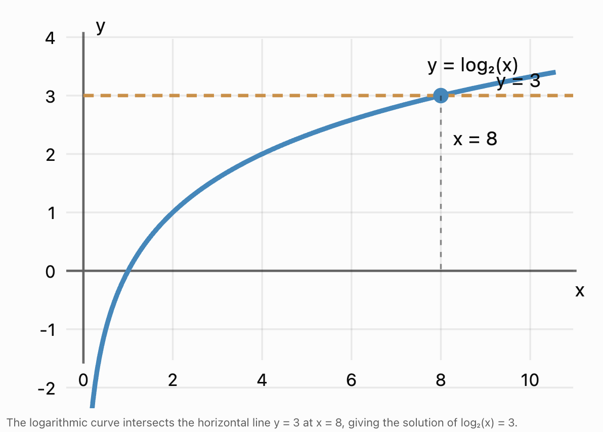
Logarithmic equations can also be solved by graphing.
Consider:
log₂(x) = 3
Graph:
y = log₂(x)
and:
y = 3
The solution is the x-coordinate of their intersection.
Advantages of Graphical Methods
Graphing can help:
-
Estimate solutions.
-
Identify the number of solutions.
-
Detect possible extraneous solutions.
-
Compare two logarithmic functions.
-
Check algebraic calculations.
For more complicated equations, a graphing calculator or mathematical software may be useful.
Numerical Solutions of Logarithmic Equations
Some logarithmic equations cannot be solved using elementary algebraic methods.
For example:
ln(x) = x − 2
The variable appears both inside and outside the logarithm.
Rearrange:
f(x) = ln(x) − x + 2
A numerical method can find values where:
f(x) = 0
This equation has two real solutions:
x ≈ 0.159 and x ≈ 3.146
These can be found using graphing technology or numerical root-finding methods.
Verification
For x ≈ 0.159:
ln(0.159) ≈ −1.839
0.159 − 2 = −1.841
The values are close.
For x ≈ 3.146:
ln(3.146) ≈ 1.146
3.146 − 2 = 1.146
Both are approximate solutions.
Practical Application: pH Calculations
The pH scale measures acidity using a logarithmic relationship.
The mathematical definition is:
pH = −log₁₀(a_H⁺)
where a_H⁺ is dimensionless hydrogen-ion activity.
In dilute aqueous solutions, activity is often approximated using concentration relative to 1 mol/L.
Worked Example
A solution has pH 4.2.
Calculate its hydrogen-ion activity.
Step 1: Write the Formula
4.2 = −log₁₀(a_H⁺)
Step 2: Multiply by −1
−4.2 = log₁₀(a_H⁺)
Step 3: Convert to Exponential Form
a_H⁺ = 10⁻⁴·²
Step 4: Calculate
a_H⁺ ≈ 6.31 × 10⁻⁵
Interpretation
The hydrogen-ion activity is approximately 6.31 × 10⁻⁵.
For a sufficiently dilute solution, this corresponds approximately to a hydrogen-ion concentration of 6.31 × 10⁻⁵ mol/L.

Practical Application: Earthquake Magnitude
A simplified logarithmic relationship for earthquake magnitude is:
M = log₁₀(A/A₀)
where:
-
M is magnitude.
-
A is corrected seismic-wave amplitude.
-
A₀ is a reference amplitude.
Actual earthquake magnitude calculations include additional measurement corrections, and modern seismology commonly uses moment magnitude.
Worked Example
An earthquake has magnitude 5.6.
Find the ratio A/A₀.
Step 1: Substitute
5.6 = log₁₀(A/A₀)
Step 2: Convert to Exponential Form
A/A₀ = 10⁵·⁶
Step 3: Calculate
A/A₀ ≈ 398107
Interpretation
The corrected amplitude is approximately 398000 times the reference amplitude in this simplified model.

Practical Application: Sound Intensity
Sound intensity level is measured using the decibel scale.
The formula is:
L = 10log₁₀(I/I₀)
where:
-
L is sound intensity level in decibels.
-
I is measured sound intensity.
-
I₀ is reference intensity.
Worked Example
A sound has an intensity level of 70 dB.
Find its intensity relative to the reference intensity.
Step 1: Substitute
70 = 10log₁₀(I/I₀)
Step 2: Divide by 10
7 = log₁₀(I/I₀)
Step 3: Convert to Exponential Form
I/I₀ = 10⁷
Final Answer
I/I₀ = 10000000
The sound intensity is ten million times the reference intensity.
If I₀ = 10⁻¹² W/m², then:
I = 10⁷ × 10⁻¹²
I = 10⁻⁵ W/m²

Practical Application: Finding Time in Growth Models
Logarithmic equations are often used to solve for time in exponential models.
Consider:
P(t) = P₀e^(kt)
where:
-
P(t) is the population at time t.
-
P₀ is the initial population.
-
k is the continuous growth rate.
-
t is time.
Worked Example
A population grows according to:
P(t) = 2000e^(0.08t)
Find when the population reaches 5000.
Step 1: Substitute
5000 = 2000e^(0.08t)
Step 2: Divide
2.5 = e^(0.08t)
Step 3: Take Natural Logarithms
ln(2.5) = 0.08t
Step 4: Solve
t = ln(2.5)/0.08
Step 5: Calculate
t ≈ 11.45
Interpretation
The population reaches 5000 after approximately 11.45 time units.
Although the unknown appears in an exponent in the original model, logarithms make it possible to solve for time.
Practical Application: Compound Interest
The compound interest formula is:
A = P(1 + r/n)^(nt)
where:
-
A is the final amount.
-
P is the initial principal.
-
r is the annual interest rate.
-
n is the number of compounding periods per year.
-
t is time in years.
Worked Example
An investment of $4000 earns 6% annual interest, compounded monthly.
How long will it take to reach $7000?
Step 1: Substitute
7000 = 4000(1 + 0.06/12)^(12t)
Step 2: Simplify
1.75 = 1.005^(12t)
Step 3: Take Natural Logarithms
ln(1.75) = 12t ln(1.005)
Step 4: Solve
t = ln(1.75)/[12ln(1.005)]
Step 5: Calculate
t ≈ 9.35 years
Interpretation
The investment reaches $7000 after approximately 9.35 years according to the continuous-time solution of the monthly-compounding formula.
Because interest is credited monthly, the balance first reaches at least $7000 after 113 complete months, or approximately 9.42 years.


A Systematic Method for Solving Logarithmic Equations
The following method works for many logarithmic equations.
Step 1: Identify the Domain
Determine the restrictions that make every logarithmic argument positive.
Step 2: Simplify the Equation
Use algebra to isolate logarithmic expressions where possible.
Step 3: Apply Logarithm Rules
Use the product, quotient, and power rules to combine or simplify logarithms.
Step 4: Convert to Exponential Form
When possible, remove the logarithm by rewriting the equation exponentially.
Step 5: Solve the Algebraic Equation
Use factoring, rearrangement, substitution, or the quadratic formula.
Step 6: Check Candidate Solutions
Reject values that violate the original domain restrictions.
Step 7: Verify in the Original Equation
Substitute each remaining candidate into the original equation.
Step 8: Interpret the Answer
For practical problems, explain the result using appropriate units and context.
Common Mistakes
Ignoring domain restrictions
Every logarithmic argument must be strictly positive.
Accepting extraneous solutions
A value obtained from algebraic manipulation is not automatically a valid logarithmic solution.
Combining logarithms incorrectly
The product rule applies to multiplication, not addition inside the argument.
Applying the quotient rule incorrectly
The difference of logarithms becomes the logarithm of a quotient.
Equating arguments with different logarithmic bases
Arguments can be equated directly only when the logarithms have the same valid base.
Forgetting the power rule
Coefficients outside logarithms can be moved into exponents.
Assuming logarithms cannot be negative
Logarithmic values may be negative even though their arguments must be positive.
Confusing logarithmic and exponential forms
Remember:
logₐ(x) = b means x = aᵇ.
Failing to verify solutions
Solutions should always be checked in the original equation.
Rounding too early
Keep exact expressions until the final calculation.
Ignoring the meaning of the result
Practical logarithmic solutions should be interpreted in context.
Key Terms
-
Logarithmic Equation: An equation containing one or more logarithmic expressions involving an unknown variable.
-
Logarithm: The exponent required to raise a base to a positive argument.
-
Base: The positive number, other than 1, used in a logarithmic expression.
-
Argument: The expression inside a logarithm.
-
Domain: The set of allowable input values.
-
Domain Restriction: A condition that limits the values a variable may take.
-
Extraneous Solution: A candidate solution that does not satisfy the original equation.
-
Verification: Checking a solution by substituting it into the original equation.
-
Exponential Form: A mathematical expression involving a base raised to a power.
-
Logarithmic Form: An equivalent expression identifying an exponent.
-
Inverse Function: A function that reverses another function.
-
Product Rule: A logarithmic property that converts multiplication into addition.
-
Quotient Rule: A logarithmic property that converts division into subtraction.
-
Power Rule: A logarithmic property that converts an exponent into a multiplier.
-
One-to-One Function: A function in which different inputs produce different outputs.
-
Natural Logarithm: A logarithm with base e.
-
Common Logarithm: A logarithm with base 10.
-
Change-of-Base Formula: A formula that rewrites a logarithm using a different base.
-
Factorisation: Rewriting an expression as a product of factors.
-
Quadratic Equation: An equation whose highest variable power is 2.
-
Quadratic Formula: A formula used to solve quadratic equations.
-
Substitution: Replacing an expression with a simpler variable.
-
Graphical Solution: A solution identified using graphs.
-
Numerical Solution: An approximate solution found through calculation.
-
Approximation: A numerical value close to an exact result.
-
pH: A logarithmic measure related to hydrogen-ion activity.
-
Earthquake Magnitude: A measure of earthquake size determined from seismic measurements.
-
Decibel: A logarithmic unit used to express ratios such as sound intensity.
-
Compound Interest: Interest calculated on an initial principal and previously accumulated interest.
-
Exponential Growth: Growth by a constant multiplicative factor over equal time intervals.
-
Mathematical Model: A mathematical representation of a real-world system.
Key Takeaways
-
Logarithmic equations contain unknown variables inside logarithmic expressions.
-
The relationship between logarithmic and exponential forms is essential for solving these equations.
-
Basic logarithmic equations can be solved by converting them into exponential form.
-
More complicated equations may require logarithmic properties and algebraic manipulation.
-
The product rule combines sums of logarithms into the logarithm of a product.
-
The quotient rule combines differences of logarithms into the logarithm of a quotient.
-
The power rule converts coefficients into exponents.
-
Logarithms with the same valid base can have their arguments equated when both arguments are positive.
-
Every logarithmic argument in the original equation must be strictly positive.
-
Domain restrictions should be identified before solving.
-
Algebraic manipulation can introduce extraneous solutions.
-
Candidate solutions must be checked against the original domain restrictions.
-
Substitution can simplify equations containing repeated logarithmic expressions.
-
Quadratic equations may arise when logarithms are combined.
-
Graphical methods help estimate solutions and determine how many solutions exist.
-
Numerical methods are useful when elementary algebraic solutions are unavailable.
-
Natural logarithms are particularly useful for models involving e.
-
Logarithmic equations are used in chemistry, geology, acoustics, finance, and population modelling.
-
Verification ensures that proposed solutions satisfy the original equation.
-
A complete logarithmic solution requires correct algebra, careful domain analysis, and verification of every candidate answer.
Check Your Understanding
Recall and Understanding
-
Explain what makes an equation a logarithmic equation.
-
Describe why logarithmic arguments must be positive.
-
Define an extraneous solution and explain how one can arise.
-
Explain when two logarithmic arguments can be equated directly.
-
Describe the difference between solving a logarithmic equation algebraically and graphically.
Application
-
Solve log₂(x) = 7.
-
Solve log₃(2x − 5) = 3.
-
Solve log₄(x + 3) = log₄(2x − 1).
-
Solve log₂(x) + log₂(x − 4) = 5, checking for extraneous solutions.
-
Solve ln(3x + 2) = 4, giving your answer to three decimal places.
Analysis and Challenge
-
Solve log₃(x + 4) − log₃(x − 2) = 2, stating the domain.
-
Solve [log₂(x)]² − 5log₂(x) + 6 = 0.
-
Solve log₂(x) + log₂(x − 1) − log₂(x + 3) = 1, checking all candidate solutions.
-
A solution has pH 3.6. Calculate its hydrogen-ion activity and explain the result.
-
An investment grows according to A = 6000(1.045)ᵗ. Determine when it reaches $10000 and explain how logarithms are used in the solution.
Final Summary
Logarithmic equations can be solved by converting logarithmic expressions into exponential form and applying appropriate algebraic techniques.
The properties of logarithms allow equations containing multiple logarithmic terms to be simplified and combined.
More advanced equations may require factoring, the quadratic formula, substitution, graphical methods, or numerical approximations.
A particularly important feature of logarithmic equations is the possibility of extraneous solutions.
Because logarithmic arguments must be positive, every candidate solution must satisfy the original domain restrictions.
Verification is essential to ensure that a calculated answer is mathematically valid.
Logarithmic equations also have important real-world applications, including pH calculations, earthquake magnitude comparisons, sound intensity measurements, compound interest, and exponential growth models.
The central principle is that solving logarithmic equations requires more than finding an algebraic answer: every solution must satisfy the original logarithmic equation and its domain restrictions.
3. Exponential Inequalities
Learning outcomes
- I can solve exponential inequalities.
- I can interpret solution intervals.
- I can represent solutions graphically.
- I can verify inequality solutions.
- I can solve practical inequality problems.
Exponential Inequalities
Introduction to Exponential Inequalities
An exponential inequality is an inequality in which the unknown variable appears in an exponent.
For example:
2ˣ > 16
This inequality asks:
"For which values of x is 2ˣ greater than 16?"
Since:
2⁴ = 16
and the function y = 2ˣ increases as x increases, we know that:
x > 4
Unlike exponential equations, which identify values that make two expressions equal, exponential inequalities identify entire sets of values that satisfy a comparison.
Exponential inequalities are useful for determining:
-
When an investment exceeds a target value.
-
When a population reaches a minimum size.
-
When radioactive material falls below a safety threshold.
-
When a bacterial population exceeds a particular limit.
-
When the value of an asset decreases below a specified amount.
-
When exponential growth or decay meets practical conditions.
Solving these inequalities requires an understanding of exponential functions, logarithms, inequality symbols, and graphical representations.


Reviewing Inequalities
An inequality compares two quantities without necessarily stating that they are equal.
The four main inequality symbols are:
|
Symbol |
Meaning |
Example |
|---|---|---|
|
> |
Greater than |
x > 3 |
|
< |
Less than |
x < 5 |
|
≥ |
Greater than or equal to |
x ≥ 2 |
|
≤ |
Less than or equal to |
x ≤ 7 |
An inequality may have infinitely many solutions.
For example:
x > 3
includes values such as:
3.1, 4, 5, 10, and 100.
However, x = 3 is not included.
By contrast:
x ≥ 3
includes x = 3 and every larger real number.
Strict and Inclusive Inequalities
Strict inequalities use:
-
Greater than (>).
-
Less than (<).
Inclusive inequalities use:
-
Greater than or equal to (≥).
-
Less than or equal to (≤).
This distinction affects whether boundary values belong to the solution set.
Understanding Exponential Functions
An exponential function has the general form:
f(x) = aˣ
where:
-
a > 0.
-
a ≠ 1.
-
x is the exponent.
The behaviour of the function depends on its base.
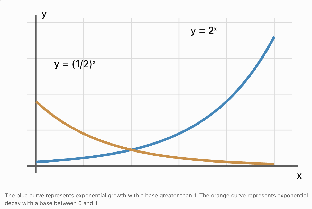
Exponential Growth
When:
a > 1
the function increases as x increases.
For example:
y = 2ˣ
|
x |
2ˣ |
|---|---|
|
−2 |
0.25 |
|
−1 |
0.5 |
|
0 |
1 |
|
1 |
2 |
|
2 |
4 |
|
3 |
8 |
|
4 |
16 |
As x increases, the output increases.
Exponential Decay
When:
0 < a < 1
the function decreases as x increases.
For example:
y = (1/2)ˣ
|
x |
(1/2)ˣ |
|---|---|
|
−2 |
4 |
|
−1 |
2 |
|
0 |
1 |
|
1 |
0.5 |
|
2 |
0.25 |
|
3 |
0.125 |
|
4 |
0.0625 |
As x increases, the output decreases.
This difference is essential when solving exponential inequalities.
Increasing and Decreasing Exponential Functions
The Fundamental Rules for Exponential Inequalities
The most important rule depends on whether the base is greater than 1 or between 0 and 1.
Rule for Bases Greater Than 1
If a > 1, then:
aᵐ > aⁿ means m > n
Similarly:
aᵐ < aⁿ means m < n
The direction of the inequality remains unchanged.
Rule for Bases Between Zero and One
If 0 < a < 1, then:
aᵐ > aⁿ means m < n
Similarly:
aᵐ < aⁿ means m > n
The direction of the inequality reverses when comparing exponents.
Why Does the Direction Reverse?
Consider:
(1/2)² = 1/4
and:
(1/2)³ = 1/8
Although:
3 > 2
we have:
1/8 < 1/4
Increasing the exponent produces a smaller output when the base lies between zero and one.
Solving Exponential Inequalities with Common Bases
The simplest exponential inequalities can be solved by expressing both sides using the same base.
Worked Example: Increasing Exponential Function
Solve:
2ˣ > 32
Step 1: Rewrite Using a Common Base
32 = 2⁵
Therefore:
2ˣ > 2⁵
Step 2: Compare Exponents
Since the base is greater than 1, the inequality direction remains unchanged.
x > 5
Step 3: Verify
Choose x = 6:
2⁶ = 64
64 > 32
The inequality is true.
Choose x = 4:
2⁴ = 16
16 > 32 is false.
Final Answer
x > 5
In interval notation:
(5, ∞)
Solving Inequalities with Algebraic Exponents
Worked Example
Solve:
3^(2x−1) ≥ 81
Step 1: Rewrite 81
81 = 3⁴
Therefore:
3^(2x−1) ≥ 3⁴
Step 2: Compare Exponents
Since 3 > 1:
2x − 1 ≥ 4
Step 3: Solve
2x ≥ 5
x ≥ 5/2
Final Answer
x ≥ 2.5
Interval notation:
[2.5, ∞)
Verification
At x = 2.5:
3^[2(2.5)−1] = 3⁴ = 81
The boundary is included because the inequality uses ≥.
Solving Inequalities with Different Bases
Sometimes both sides can be rewritten using a common base.
Worked Example
Solve:
4ˣ < 8^(x−1)
Step 1: Rewrite Using Base 2
4 = 2²
8 = 2³
Therefore:
2^(2x) < 2^(3x−3)
Step 2: Compare Exponents
Since 2 > 1:
2x < 3x − 3
Step 3: Solve
3 < x
Final Answer
x > 3
Interval notation:
(3, ∞)
Verification
Choose x = 4:
Left side:
4⁴ = 256
Right side:
8³ = 512
Since:
256 < 512
the inequality is true.
Solving Inequalities with Bases Between Zero and One
When the base lies between zero and one, the exponential function is decreasing.
This means the inequality direction reverses when comparing exponents.
Worked Example
Solve:
(1/2)ˣ > 1/16
Step 1: Rewrite the Right Side
1/16 = (1/2)⁴
Therefore:
(1/2)ˣ > (1/2)⁴
Step 2: Compare Exponents
Because:
0 < 1/2 < 1
the inequality direction reverses.
x < 4
Step 3: Verify
Choose x = 3:
(1/2)³ = 1/8
Since:
1/8 > 1/16
the inequality is true.
Choose x = 5:
(1/2)⁵ = 1/32
Since:
1/32 < 1/16
the inequality is false.
Final Answer
x < 4
Interval notation:
(−∞, 4)
Inequalities with Algebraic Exponents and Fractional Bases
Worked Example
Solve:
(1/3)^(2x+1) ≤ 1/27
Step 1: Rewrite the Right Side
1/27 = (1/3)³
Therefore:
(1/3)^(2x+1) ≤ (1/3)³
Step 2: Reverse the Inequality
Because the base lies between zero and one:
2x + 1 ≥ 3
Step 3: Solve
2x ≥ 2
x ≥ 1
Final Answer
x ≥ 1
Interval notation:
[1, ∞)
Verification
At x = 1:
(1/3)³ = 1/27
Equality holds, so the boundary is included.
Solving Exponential Inequalities Using Logarithms
Not every exponential inequality can be rewritten using common bases.
Consider:
2ˣ > 15
Since 15 is not a convenient power of 2, logarithms are useful.
Important Logarithmic Principle
The natural logarithm is a strictly increasing function.
Therefore, for positive A and B:
A > B means ln(A) > ln(B)
Taking natural logarithms of two positive expressions preserves the inequality direction.
However, when dividing by a negative logarithmic value, the inequality must reverse.
Worked Example: Using Logarithms
Solve:
2ˣ > 15
Step 1: Take Natural Logarithms
ln(2ˣ) > ln(15)
Step 2: Apply the Power Rule
x ln(2) > ln(15)
Step 3: Divide
Since ln(2) > 0, the inequality direction remains unchanged.
x > ln(15)/ln(2)
Step 4: Calculate
x > 3.907
Final Answer
Exact form:
x > ln(15)/ln(2)
Approximate interval:
(3.907, ∞)
The exact logarithmic boundary is preferable when precision matters.
Worked Example: Logarithms with Algebraic Exponents
Solve:
5^(2x−3) ≤ 40
Step 1: Take Natural Logarithms
ln[5^(2x−3)] ≤ ln(40)
Step 2: Apply the Power Rule
(2x − 3)ln(5) ≤ ln(40)
Step 3: Divide by ln(5)
Since ln(5) > 0:
2x − 3 ≤ ln(40)/ln(5)
Step 4: Solve
2x ≤ 3 + ln(40)/ln(5)
x ≤ [3 + ln(40)/ln(5)]/2
Step 5: Calculate
x ≤ 2.646
Final Answer
Approximately:
(−∞, 2.646]
Logarithms with Bases Between Zero and One
Worked Example
Solve:
0.8ˣ > 0.3
Step 1: Take Natural Logarithms
ln(0.8ˣ) > ln(0.3)
Step 2: Apply the Power Rule
x ln(0.8) > ln(0.3)
Step 3: Examine the Sign
Since:
ln(0.8) < 0
dividing by ln(0.8) reverses the inequality.
Therefore:
x < ln(0.3)/ln(0.8)
Step 4: Calculate
x < 5.396
Final Answer
Approximately:
(−∞, 5.396)
Verification
Choose x = 5:
0.8⁵ = 0.32768
0.32768 > 0.3
The inequality is true.
Choose x = 6:
0.8⁶ = 0.262144
0.262144 > 0.3 is false.
This confirms the solution boundary.
Representing Solutions Using Interval Notation
Interval notation is a compact way to describe solution sets.
Parentheses
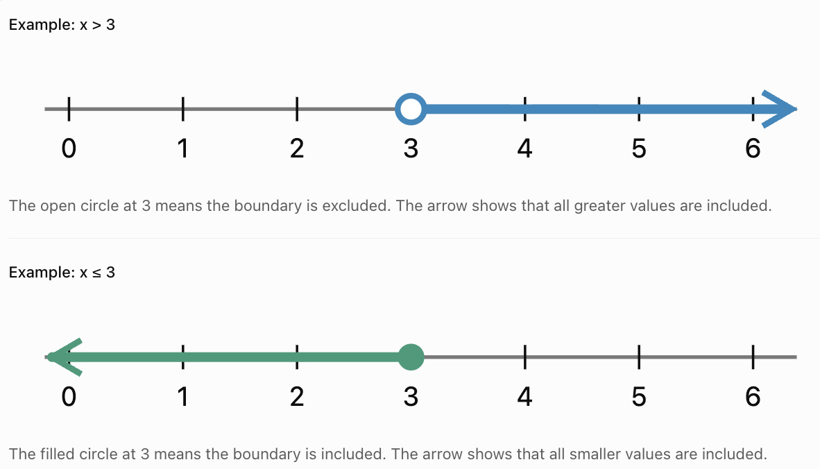
Parentheses indicate that a boundary is excluded.
For example:
x > 4
becomes:
(4, ∞)
Square Brackets
Square brackets indicate that a finite boundary is included.
For example:
x ≥ 4
becomes:
[4, ∞)
Common Interval Forms
|
Inequality |
Interval notation |
|---|---|
|
x > 3 |
(3, ∞) |
|
x ≥ 3 |
[3, ∞) |
|
x < 5 |
(−∞, 5) |
|
x ≤ 5 |
(−∞, 5] |
|
2 < x < 7 |
(2, 7) |
|
2 ≤ x ≤ 7 |
[2, 7] |
|
x ≤ 1 or x ≥ 4 |
(−∞, 1] ∪ [4, ∞) |
Important Rules
-
Parentheses exclude boundary values.
-
Square brackets include finite boundary values.
-
Infinity always uses parentheses.
-
The union symbol ∪ combines separate intervals.
Representing Solutions on Number Lines
A number line helps show which values satisfy an inequality.
Graph:
y = 2ˣ
and:
y = 8
The curves intersect when:
2ˣ = 8
Therefore:
x = 3
For x > 3, the exponential curve lies above the horizontal line.
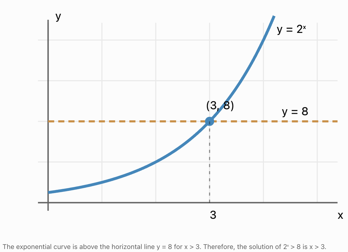
Graphical Interpretation
-
Above the comparison curve: the exponential expression is greater.
-
Below the comparison curve: the exponential expression is smaller.
-
At an intersection: the expressions are equal.
For strict inequalities, intersection points are excluded.
For inclusive inequalities, intersection points are included.
Solving Compound Exponential Inequalities
A compound inequality contains two comparisons.
For example:
4 ≤ 2ˣ < 32
Worked Example
Solve:
4 ≤ 2ˣ < 32
Step 1: Rewrite Using Base 2
4 = 2²
32 = 2⁵
Therefore:
2² ≤ 2ˣ < 2⁵
Step 2: Compare Exponents
Since 2 > 1:
2 ≤ x < 5
Final Answer
Interval notation:
[2, 5)
Interpretation
The solution includes x = 2 but excludes x = 5.
Compound Inequalities with Decay Functions
Worked Example
Solve:
1/16 < (1/2)ˣ ≤ 1/4
Step 1: Rewrite Using a Common Base
1/16 = (1/2)⁴
1/4 = (1/2)²
Therefore:
(1/2)⁴ < (1/2)ˣ ≤ (1/2)²
Step 2: Reverse Both Inequality Directions
Because the base is between zero and one:
4 > x ≥ 2
Rearrange:
2 ≤ x < 4
Final Answer
[2, 4)
Exponential Inequalities with Multiple Terms
Some exponential inequalities can be solved using substitution.
Consider:
2^(2x) − 5(2ˣ) + 4 > 0
Step 1: Substitute
Let:
u = 2ˣ
Since 2ˣ > 0:
u > 0
Also:
2^(2x) = u²
The inequality becomes:
u² − 5u + 4 > 0
Step 2: Factorise
(u − 1)(u − 4) > 0
Step 3: Solve the Quadratic Inequality
The product is positive when both factors have the same sign.
Therefore:
u < 1
or:
u > 4
But u > 0, so:
0 < u < 1 or u > 4
Step 4: Substitute Back
2ˣ < 1
or:
2ˣ > 4
Step 5: Solve
Since:
1 = 2⁰
and:
4 = 2²
we obtain:
x < 0 or x > 2
Final Answer
Interval notation:
(−∞, 0) ∪ (2, ∞)
Verification
Choose x = −1:
2⁻² − 5(2⁻¹) + 4
= 0.25 − 2.5 + 4
= 1.75 > 0
Choose x = 1:
2² − 5(2) + 4
= 4 − 10 + 4
= −2
This does not satisfy the inequality.
Choose x = 3:
2⁶ − 5(8) + 4
= 64 − 40 + 4
= 28 > 0
The two solution intervals are confirmed.
Using Sign Analysis
When an exponential inequality becomes a quadratic inequality, a sign chart can help determine where the expression is positive or negative.
For:
(u − 1)(u − 4) > 0
the critical values are:
u = 1
u = 4
|
Interval |
Sign of u − 1 |
Sign of u − 4 |
Product |
|---|---|---|---|
|
u < 1 |
Negative |
Negative |
Positive |
|
1 < u < 4 |
Positive |
Negative |
Negative |
|
u > 4 |
Positive |
Positive |
Positive |
This approach is especially useful for more complicated exponential inequalities.
Practical Application: Compound Interest
Exponential inequalities can determine when an investment exceeds a financial target.
The compound interest formula is:
A = P(1 + r/n)^(nt)
where:
-
A = final amount.
-
P = initial investment.
-
r = annual interest rate as a decimal.
-
n = number of compounding periods per year.
-
t = time in years.
Worked Example
An investment of $5000 earns 6% annual interest, compounded annually.
When will the investment exceed $8000?
Step 1: Write the Inequality
5000(1.06)ᵗ > 8000
Step 2: Divide
1.06ᵗ > 1.6
Step 3: Take Natural Logarithms
t ln(1.06) > ln(1.6)
Step 4: Solve
Since ln(1.06) > 0:
t > ln(1.6)/ln(1.06)
Step 5: Calculate
t > 8.066 years
Interpretation
The model exceeds $8000 after approximately 8.07 years.
Since interest is compounded annually, the account first exceeds $8000 after 9 complete years.

Practical Application: Population Growth
Suppose a population increases by 5% each year.
The model is:
P(t) = P₀(1.05)ᵗ
Worked Example
A town has an initial population of 15000.
When will its population exceed 25000?
Step 1: Write the Inequality
15000(1.05)ᵗ > 25000
Step 2: Divide
1.05ᵗ > 5/3
Step 3: Take Logarithms
t ln(1.05) > ln(5/3)
Step 4: Solve
t > ln(5/3)/ln(1.05)
Step 5: Calculate
t > 10.47 years
Interpretation
The model predicts that the population exceeds 25000 after approximately 10.47 years.
If population values are evaluated only at the end of each year, the first qualifying year is year 11.
Practical Application: Radioactive Decay
Radioactive decay is commonly modelled using:
N(t) = N₀e^(−λt)
where:
-
N(t) = amount remaining.
-
N₀ = initial amount.
-
λ = decay constant.
-
t = time.
Worked Example
A radioactive substance has an initial mass of 200 g and a decay constant of 0.08 per year.
When will its mass fall below 50 g?
Step 1: Write the Inequality
200e^(−0.08t) < 50
Step 2: Divide
e^(−0.08t) < 0.25
Step 3: Take Natural Logarithms
−0.08t < ln(0.25)
Step 4: Divide by a Negative Number
Dividing by −0.08 reverses the inequality.
t > ln(0.25)/(−0.08)
Step 5: Calculate
t > 17.33 years
Interpretation
The mass falls below 50 g after approximately 17.33 years.
At exactly the threshold time, the mass equals 50 g. Because the inequality is strict, that boundary is excluded.


Practical Application: Bacterial Growth
A bacterial population doubles every 4 hours.
The population model is:
N(t) = 300 × 2^(t/4)
where t is measured in hours.
Worked Example
When will the population exceed 5000 bacteria?
Step 1: Write the Inequality
300 × 2^(t/4) > 5000
Step 2: Divide
2^(t/4) > 5000/300
2^(t/4) > 50/3
Step 3: Take Logarithms
(t/4)ln(2) > ln(50/3)
Step 4: Solve
t > 4ln(50/3)/ln(2)
Step 5: Calculate
t > 16.24 hours
Interpretation
Under the exponential model, the population exceeds 5000 after approximately 16.24 hours.
If the model instead represents discrete doubling events occurring only every 4 hours, the first event producing more than 5000 bacteria occurs at 20 hours.
Practical Application: Depreciation
A vehicle loses 12% of its value each year.
Its value is modelled by:
V(t) = 30000(0.88)ᵗ
Worked Example
When will the vehicle be worth less than $15000?
Step 1: Write the Inequality
30000(0.88)ᵗ < 15000
Step 2: Divide
0.88ᵗ < 0.5
Step 3: Take Natural Logarithms
t ln(0.88) < ln(0.5)
Step 4: Divide by a Negative Value
Since:
ln(0.88) < 0
the inequality reverses.
t > ln(0.5)/ln(0.88)
Step 5: Calculate
t > 5.42 years
Interpretation
The model predicts that the vehicle's value falls below $15000 after approximately 5.42 years.
If depreciation is applied only at the end of each year, the value first falls below $15000 after 6 complete years.
Verifying Exponential Inequalities
Verification helps determine whether a proposed solution interval is correct.
Unlike an equation, an inequality may have infinitely many solutions.
Therefore, checking one value does not prove the entire interval is correct.
However, testing values from different regions can help detect errors.
Verification Strategy
-
Identify the boundary value.
-
Determine whether the boundary should be included.
-
Choose a test value inside the proposed solution interval.
-
Substitute into the original inequality.
-
Choose a test value outside the proposed solution interval.
-
Confirm that the inequality is false outside the solution set.
-
Use the function's monotonicity or a sign chart to justify the complete interval.
Worked Example
Verify:
3ˣ ≥ 27
Proposed solution:
x ≥ 3
Boundary Check
At x = 3:
3³ = 27
The inequality is true.
Test a Larger Value
At x = 4:
3⁴ = 81
81 ≥ 27
True.
Test a Smaller Value
At x = 2:
3² = 9
9 ≥ 27
False.
Since 3ˣ is strictly increasing, these checks agree with the full solution:
x ≥ 3
Choosing the Best Method
|
Inequality type |
Recommended method |
|---|---|
|
2ˣ > 32 |
Common bases |
|
3^(2x−1) ≥ 81 |
Common bases and algebra |
|
4ˣ < 8^(x−1) |
Rewrite using a common base |
|
(1/2)ˣ > 1/16 |
Common bases with reversed inequality |
|
2ˣ > 15 |
Logarithms |
|
5^(2x−3) ≤ 40 |
Logarithms and algebra |
|
0.8ˣ > 0.3 |
Logarithms with a negative divisor |
|
4 ≤ 2ˣ < 32 |
Compound inequality |
|
2^(2x) − 5(2ˣ) + 4 > 0 |
Substitution and sign analysis |
|
2ˣ > x + 3 |
Graphical or numerical analysis |
The most efficient method depends on the structure of the inequality.
Common Mistakes
Forgetting to reverse an inequality when dividing by a negative number
This is particularly important when working with logarithms of bases between zero and one.
Treating exponential growth and decay in the same way
Increasing and decreasing exponential functions behave differently.
Equating exponents when bases are different
The bases must first be made equal or logarithms must be used.
Using logarithms without checking positivity
Logarithms can only be applied to positive real quantities.
Ignoring strict versus inclusive inequalities
The symbols > and ≥ produce different solution sets.
Using the wrong interval brackets
Parentheses exclude finite boundary values, while square brackets include them.
Including infinity as a boundary value
Infinity is not a real number and always uses parentheses.
Failing to check transformed quadratic inequalities
Factoring produces critical points, but sign analysis is needed to identify valid intervals.
Ignoring positivity after exponential substitution
If u = aˣ, then u > 0.
Rounding boundaries too early
An approximate boundary may incorrectly include or exclude values close to the true solution.
Assuming one test value proves the complete solution
Testing helps verify a result, but monotonicity or sign analysis provides the mathematical justification.
Ignoring practical constraints
Time, population, and financial quantities may require nonnegative values or discrete reporting intervals.
Key Terms
-
Exponential Inequality: An inequality containing an unknown variable in an exponent.
-
Inequality: A mathematical comparison using symbols such as >, <, ≥, or ≤.
-
Solution Set: The collection of values satisfying an inequality.
-
Boundary Value: A value where the compared expressions are equal.
-
Strict Inequality: An inequality that excludes equality.
-
Inclusive Inequality: An inequality that allows equality.
-
Exponential Function: A function in which the variable appears in an exponent.
-
Exponential Growth: An exponential relationship that increases as the independent variable increases.
-
Exponential Decay: An exponential relationship that decreases as the independent variable increases.
-
Increasing Function: A function whose output increases as its input increases.
-
Decreasing Function: A function whose output decreases as its input increases.
-
Monotonic Function: A function that consistently increases or consistently decreases over an interval.
-
Common Base: A shared base used to compare exponential expressions.
-
Logarithm: The exponent required to produce a specified positive value from a given base.
-
Natural Logarithm: A logarithm with base e.
-
Change-of-Base Formula: A formula used to rewrite logarithms using another valid base.
-
Interval Notation: A notation used to describe sets of real numbers.
-
Open Interval: An interval that excludes its finite endpoints.
-
Closed Interval: An interval that includes both finite endpoints.
-
Union: A combination of two or more sets.
-
Number Line: A visual representation of real numbers and intervals.
-
Graphical Solution: A solution determined by comparing mathematical graphs.
-
Intersection Point: A point where two graphs have equal coordinates.
-
Compound Inequality: An inequality involving more than one comparison.
-
Substitution: Replacing a complicated expression with a simpler variable.
-
Quadratic Inequality: An inequality involving a quadratic expression.
-
Critical Value: A value where an expression becomes zero or otherwise changes its sign behaviour.
-
Sign Chart: A method for identifying intervals where an expression is positive or negative.
-
Verification: Checking whether values satisfy the original inequality.
-
Threshold: A boundary value used to determine whether a condition has been reached.
-
Compound Interest: Interest calculated on an initial principal and accumulated interest.
-
Decay Constant: A parameter describing continuous exponential decay.
-
Depreciation: A decrease in the value of an asset over time.
-
Mathematical Model: A mathematical representation of a real-world process.
Key Takeaways
-
Exponential inequalities identify sets of values rather than individual equality solutions.
-
Exponential inequalities can often be solved by expressing both sides using a common base.
-
For bases greater than 1, exponential functions are increasing.
-
When comparing exponents with a base greater than 1, the inequality direction remains unchanged.
-
For bases between zero and one, exponential functions are decreasing.
-
When comparing exponents with a base between zero and one, the inequality direction reverses.
-
Logarithms are useful when exponential expressions cannot be rewritten using convenient common bases.
-
Natural logarithms preserve inequalities between positive arguments because ln(x) is increasing.
-
Dividing an inequality by a negative logarithmic value reverses its direction.
-
Strict inequalities exclude boundary values.
-
Inclusive inequalities include boundary values.
-
Interval notation provides a compact representation of solution sets.
-
Number lines visually distinguish included and excluded boundary values.
-
Graphical solutions identify where one function lies above or below another.
-
Compound exponential inequalities can produce bounded intervals.
-
Some exponential inequalities can be transformed into quadratic inequalities using substitution.
-
Sign charts help identify valid intervals for transformed polynomial inequalities.
-
Verification should include boundary checks and test values from relevant intervals.
-
Exponential inequalities are used to determine when growth or decay processes cross specified thresholds.
-
Practical applications include investments, population growth, radioactive decay, bacterial growth, and depreciation.
-
Mathematical models should be interpreted using appropriate units and real-world constraints.
-
The most important skill is recognising whether the exponential function is increasing or decreasing, because this determines the correct inequality direction.
Check Your Understanding
Recall and Understanding
-
Explain the difference between an exponential equation and an exponential inequality.
-
State the rule for comparing exponential expressions with bases greater than 1.
-
Explain why inequality directions reverse when comparing powers of a base between zero and one.
-
Describe the difference between open and closed intervals.
-
Explain how a graph can be used to solve an exponential inequality.
Application
-
Solve 2ˣ > 64 and express the answer in interval notation.
-
Solve 3^(2x−1) ≤ 243.
-
Solve (1/2)ˣ ≥ 1/32.
-
Solve 5ˣ > 70, giving the boundary to three decimal places.
-
Solve 4 ≤ 2ˣ < 64 and represent the solution using interval notation.
Analysis and Challenge
-
Solve 4ˣ > 8^(x−2), showing how common bases are used.
-
Solve 0.7ˣ ≤ 0.2, explaining why the inequality direction changes.
-
Solve 2^(2x) − 6(2ˣ) + 8 ≥ 0 using substitution and sign analysis.
-
An investment of $8000 grows at 5% annually, compounded annually. Determine when its value first exceeds $12000.
-
A radioactive substance has an initial mass of 500 g and follows N(t) = 500e^(−0.06t). Determine when its mass falls below 100 g, giving the solution as an inequality and interpreting the result.
Final Summary
Exponential inequalities are used to determine the values of a variable for which an exponential expression is greater than, less than, or equal to a specified quantity.
The most important distinction is between exponential growth and exponential decay.
When the base is greater than 1, the exponential function increases and the inequality direction remains unchanged when comparing exponents.
When the base lies between zero and one, the exponential function decreases and the inequality direction reverses.
Logarithms allow more complicated exponential inequalities to be solved when common bases are unavailable.
Solutions can be expressed using inequality notation, interval notation, number lines, and graphs.
More advanced inequalities may require substitution and sign analysis to identify multiple solution intervals.
Exponential inequalities are especially useful for solving real-world threshold problems involving growth, decay, finance, biology, and environmental science.
The central principle is that exponential inequalities are solved by combining the properties of exponential functions with correct inequality operations, careful interval interpretation, and verification of the resulting solution set.
4. Logarithmic Inequalities
Learning outcomes
- I can solve logarithmic inequalities.
- I can identify domain restrictions.
- I can interpret solution sets.
- I can verify logarithmic inequalities.
- I can solve contextual problems.
Logarithmic Inequalities
Introduction to Logarithmic Inequalities
A logarithmic inequality is an inequality in which the unknown variable appears inside a logarithmic expression.
For example:
log₂(x) > 3
This inequality asks:
"For which values of x is the logarithm of x to base 2 greater than 3?"
Since:
log₂(8) = 3
and log₂(x) increases as x increases, the solution is:
x > 8
Unlike logarithmic equations, which usually identify specific values, logarithmic inequalities identify entire intervals of values that satisfy a condition.
Solving logarithmic inequalities involves several important mathematical ideas:
-
Understanding whether a logarithmic function is increasing or decreasing.
-
Identifying domain restrictions.
-
Applying logarithmic properties correctly.
-
Converting logarithmic inequalities into algebraic inequalities.
-
Representing solution sets using interval notation.
-
Verifying solutions and rejecting invalid values.
-
Applying logarithmic inequalities to real-world situations.
Logarithmic inequalities are useful in chemistry, physics, finance, engineering, and environmental science, particularly when quantities are measured using logarithmic scales.


Reviewing Logarithmic Functions
A logarithmic function has the general form:
f(x) = logₐ(x)
where:
-
a is the base.
-
x is the argument.
-
a > 0.
-
a ≠ 1.
-
x > 0.
Logarithms are inverse functions of exponentials.
The relationship is:
logₐ(x) = y ⇔ aʸ = x
For example:
log₂(16) = 4
because:
2⁴ = 16
This relationship allows logarithmic inequalities to be converted into exponential or algebraic inequalities.
Increasing and Decreasing Logarithmic Functions
The direction of a logarithmic inequality depends on the base.
Bases Greater Than One
When:
a > 1
the logarithmic function is increasing.
Examples include:
-
log₂(x)
-
log₃(x)
-
log₁₀(x)
-
ln(x)
As x increases, the logarithmic value increases.
Bases Between Zero and One
When:
0 < a < 1
the logarithmic function is decreasing.
Examples include:
-
log₁/₂(x)
-
log₁/₃(x)
-
log₀.₈(x)
As x increases, the logarithmic value decreases.
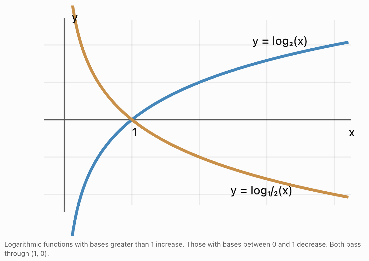
Fundamental Rules for Logarithmic Inequalities
Rule for Bases Greater Than One
For positive M and N, when a > 1:
logₐ(M) > logₐ(N) ⇔ M > N
The inequality direction remains unchanged.
Similarly:
logₐ(M) ≤ logₐ(N) ⇔ M ≤ N
Rule for Bases Between Zero and One
For positive M and N, when 0 < a < 1:
logₐ(M) > logₐ(N) ⇔ M < N
The inequality direction reverses.
Similarly:
logₐ(M) ≤ logₐ(N) ⇔ M ≥ N
Why Does the Inequality Reverse?
Consider:
log₁/₂(2) = −1
and:
log₁/₂(4) = −2
Although:
4 > 2
we have:
−2 < −1
Therefore:
log₁/₂(4) < log₁/₂(2)
The logarithmic function decreases as its argument increases.
Domain Restrictions
One of the most important differences between ordinary algebraic inequalities and logarithmic inequalities is the restriction on logarithmic arguments.
The argument of every real logarithm must be strictly positive.
For:
log₂(x)
the domain is:
x > 0
For:
log₃(x − 4)
the domain is:
x > 4
For:
ln(7 − x)
the domain is:
x < 7
A proposed solution that violates any original logarithmic domain restriction must be rejected.
Finding Domain Restrictions
Example: Linear Argument
Find the domain of:
log₂(3x − 6)
Require:
3x − 6 > 0
3x > 6
x > 2
Example: Negative Coefficient
Find the domain of:
ln(10 − 2x)
Require:
10 − 2x > 0
−2x > −10
Divide by −2 and reverse the inequality:
x < 5
Example: Quadratic Argument
Find the domain of:
log₃(x² − 9)
Require:
x² − 9 > 0
Factorise:
(x − 3)(x + 3) > 0
The product is positive when:
x < −3
or:
x > 3
Therefore, the domain is:
(−∞, −3) ∪ (3, ∞)
Important Observation
Logarithmic domains are not always single intervals.
A logarithm with a quadratic or rational argument may have several disconnected parts of its domain.
Solving Basic Logarithmic Inequalities
The simplest logarithmic inequalities contain one logarithm compared with a constant.
Worked Example: Base Greater Than One
Solve:
log₂(x) > 4
Step 1: Identify the Domain
x > 0
Step 2: Convert to Exponential Form
Since the base is greater than 1:
x > 2⁴
Step 3: Simplify
x > 16
Step 4: Check the Domain
Every value greater than 16 is positive.
Final Answer
x > 16
Interval notation:
(16, ∞)
Verification
Choose x = 32:
log₂(32) = 5
5 > 4
True.
Choose x = 8:
log₂(8) = 3
3 > 4 is false.
The solution is consistent.
Solving Inclusive Logarithmic Inequalities
Worked Example
Solve:
log₃(x) ≤ 2
Step 1: Identify the Domain
x > 0
Step 2: Convert to Exponential Form
Since 3 > 1:
x ≤ 3²
Step 3: Simplify
x ≤ 9
Step 4: Combine with the Domain
The logarithm requires x > 0.
Therefore:
0 < x ≤ 9
Final Answer
(0, 9]
Important Observation
Although the algebra gives x ≤ 9, the logarithmic domain excludes zero and all negative values.
This is why domain restrictions must always be included in the final solution.
Solving Inequalities with Algebraic Arguments
Worked Example
Solve:
log₅(2x − 1) ≥ 2
Step 1: Find the Domain
2x − 1 > 0
x > 1/2
Step 2: Convert to Exponential Form
Since 5 > 1:
2x − 1 ≥ 5²
Step 3: Simplify
2x − 1 ≥ 25
2x ≥ 26
x ≥ 13
Step 4: Check the Domain
All values x ≥ 13 satisfy x > 1/2.
Final Answer
[13, ∞)
Solving Inequalities with Decreasing Logarithms
Worked Example
Solve:
log₁/₂(x) > 3
Step 1: Identify the Domain
x > 0
Step 2: Reverse the Inequality
Because the base is between zero and one:
x < (1/2)³
Step 3: Simplify
x < 1/8
Step 4: Combine with the Domain
0 < x < 1/8
Final Answer
(0, 1/8)
Verification
Choose x = 1/16:
log₁/₂(1/16) = 4
4 > 3
True.
Choose x = 1/4:
log₁/₂(1/4) = 2
2 > 3 is false.
Another Example with a Fractional Base
Solve:
log₁/₃(2x + 1) ≤ −2
Step 1: Identify the Domain
2x + 1 > 0
x > −1/2
Step 2: Reverse the Inequality
Because 0 < 1/3 < 1:
2x + 1 ≥ (1/3)⁻²
Step 3: Evaluate
(1/3)⁻² = 9
Therefore:
2x + 1 ≥ 9
2x ≥ 8
x ≥ 4
Step 4: Check the Domain
The solution satisfies x > −1/2.
Final Answer
[4, ∞)
Solving Logarithmic Inequalities with Logarithms on Both Sides
When two logarithms have the same base, their arguments can be compared directly, provided both arguments are positive.
Worked Example
Solve:
log₃(2x + 1) > log₃(x + 5)
Step 1: Identify Domain Restrictions
2x + 1 > 0
x > −1/2
Also:
x + 5 > 0
x > −5
Combined domain:
x > −1/2
Step 2: Compare Arguments
Since 3 > 1:
2x + 1 > x + 5
Step 3: Solve
x > 4
Step 4: Check the Domain
All values greater than 4 satisfy the original domain restrictions.
Final Answer
(4, ∞)
Comparing Logarithms with a Decreasing Base
Worked Example
Solve:
log₁/₂(x + 3) ≥ log₁/₂(2x − 1)
Step 1: Find the Domain
x + 3 > 0
x > −3
Also:
2x − 1 > 0
x > 1/2
Combined domain:
x > 1/2
Step 2: Reverse the Inequality
Since the base is between zero and one:
x + 3 ≤ 2x − 1
Step 3: Solve
4 ≤ x
x ≥ 4
Step 4: Check the Domain
All values x ≥ 4 are valid.
Final Answer
[4, ∞)
Solving Inequalities with Multiple Logarithms
Some logarithmic inequalities contain sums or differences of logarithmic expressions.
These can often be simplified using logarithmic properties.
Product Rule
logₐ(M) + logₐ(N) = logₐ(MN)
Quotient Rule
logₐ(M) − logₐ(N) = logₐ(M/N)
Power Rule
klogₐ(M) = logₐ(Mᵏ)
These rules must be applied while preserving the domain restrictions of the original expressions.
Using the Product Rule
Worked Example
Solve:
log₂(x) + log₂(x − 2) > 3
Step 1: Find the Domain
x > 0
x − 2 > 0
Therefore:
x > 2
Step 2: Combine Logarithms
log₂[x(x − 2)] > 3
Step 3: Convert to an Algebraic Inequality
Since 2 > 1:
x(x − 2) > 2³
x(x − 2) > 8
Step 4: Expand
x² − 2x > 8
x² − 2x − 8 > 0
Step 5: Factorise
(x − 4)(x + 2) > 0
Step 6: Solve the Quadratic Inequality
The product is positive when:
x < −2
or:
x > 4
Step 7: Apply the Domain
The original logarithms require x > 2.
Therefore, x < −2 is invalid.
Final Answer
x > 4
Interval notation:
(4, ∞)
Verification
Choose x = 6:
log₂(6) + log₂(4)
= log₂(24)
≈ 4.585
Since 4.585 > 3, the inequality is true.
Choose x = 3:
log₂(3) + log₂(1)
≈ 1.585
The inequality is false.
Using the Quotient Rule
Worked Example
Solve:
log₃(x + 4) − log₃(x − 2) ≥ 1
Step 1: Identify the Domain
x + 4 > 0
x − 2 > 0
Therefore:
x > 2
Step 2: Apply the Quotient Rule
log₃[(x + 4)/(x − 2)] ≥ 1
Step 3: Convert to an Algebraic Inequality
Since 3 > 1:
(x + 4)/(x − 2) ≥ 3
Step 4: Use the Domain
Because x > 2, the denominator x − 2 is positive.
We can multiply both sides without reversing the inequality:
x + 4 ≥ 3(x − 2)
Step 5: Expand
x + 4 ≥ 3x − 6
10 ≥ 2x
x ≤ 5
Step 6: Combine with the Domain
x > 2
and:
x ≤ 5
Final Answer
2 < x ≤ 5
Interval notation:
(2, 5]
Important Principle
When multiplying an inequality by an expression containing x, determine whether that expression is positive or negative.
The sign determines whether the inequality direction remains unchanged or reverses.
Using the Power Rule
Worked Example
Solve:
2log₂(x) ≤ 6
Step 1: Identify the Domain
x > 0
Step 2: Divide by 2
log₂(x) ≤ 3
Step 3: Convert to Exponential Form
x ≤ 2³
x ≤ 8
Step 4: Combine with the Domain
0 < x ≤ 8
Final Answer
(0, 8]
Logarithmic Inequalities with Quadratic Expressions
More complicated inequalities may produce quadratic expressions.
These require factoring or the quadratic formula, followed by sign analysis.
Worked Example
Solve:
log₂(x² − 5x + 6) > 1
Step 1: Identify the Domain
x² − 5x + 6 > 0
Factorise:
(x − 2)(x − 3) > 0
Therefore, the domain is:
x < 2 or x > 3
Step 2: Convert the Logarithmic Inequality
Since 2 > 1:
x² − 5x + 6 > 2¹
Step 3: Simplify
x² − 5x + 6 > 2
x² − 5x + 4 > 0
Step 4: Factorise
(x − 1)(x − 4) > 0
Step 5: Solve the Quadratic Inequality
The product is positive when:
x < 1
or:
x > 4
Step 6: Check the Domain
Both intervals lie within the original domain.
Final Answer
x < 1 or x > 4
Interval notation:
(−∞, 1) ∪ (4, ∞)
Interpretation
The inequality has two separate solution intervals.
This happens because the quadratic argument is large enough on both sides of its central region.
Sign Charts and Logarithmic Inequalities
Sign charts help identify intervals where polynomial or rational expressions are positive or negative.
Consider:
(x − 1)(x − 4) > 0
The critical values are:
x = 1
x = 4
|
Interval |
Sign of x − 1 |
Sign of x − 4 |
Product |
|---|---|---|---|
|
x < 1 |
Negative |
Negative |
Positive |
|
1 < x < 4 |
Positive |
Negative |
Negative |
|
x > 4 |
Positive |
Positive |
Positive |
The product is positive outside the two critical values.
Therefore:
x < 1 or x > 4
Sign charts are particularly useful when inequalities contain several factors.
Interpreting Solution Sets
A logarithmic inequality may have:
-
One bounded interval.
-
One unbounded interval.
-
Two or more separate intervals.
-
All values in its domain.
-
No real solutions.
The solution set must satisfy both the logarithmic comparison and all domain restrictions.
Interval Notation
|
Inequality |
Interval notation |
|---|---|
|
x > 3 |
(3, ∞) |
|
x ≥ 3 |
[3, ∞) |
|
x < 5 |
(−∞, 5) |
|
x ≤ 5 |
(−∞, 5] |
|
2 < x < 7 |
(2, 7) |
|
2 ≤ x ≤ 7 |
[2, 7] |
|
x < 1 or x > 4 |
(−∞, 1) ∪ (4, ∞) |
Open and Closed Boundaries
An open boundary excludes the endpoint.
A closed boundary includes the endpoint.
However, a logarithmic domain boundary is always excluded when the argument becomes zero.
For example:
log₂(x − 3) ≥ 0
requires x > 3.
The solution is:
x − 3 ≥ 1
x ≥ 4
Therefore:
[4, ∞)
The boundary x = 4 is included because the logarithm is defined there and the inequality permits equality.
Representing Solutions on Number Lines
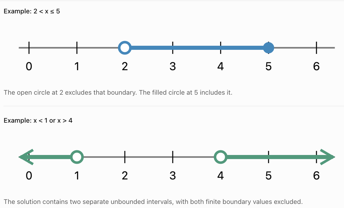
Graphical Solutions of Logarithmic Inequalities
Logarithmic inequalities can also be solved by comparing graphs.
Consider:
log₂(x) > 2
Graph:
y = log₂(x)
and:
y = 2
The graphs intersect when:
log₂(x) = 2
Therefore:
x = 4
For x > 4, the logarithmic curve lies above the horizontal line.
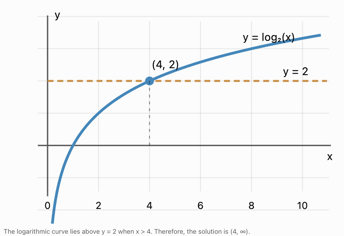
Advantages of Graphical Methods
Graphs can help:
-
Identify solution intervals.
-
Estimate boundary values.
-
Show whether a function is increasing or decreasing.
-
Compare logarithmic expressions.
-
Identify multiple solution regions.
-
Verify algebraic answers.
Graphical methods are particularly useful when exact algebraic solutions are difficult.
Verifying Logarithmic Inequalities
Verification is essential because algebraic manipulation may produce intervals containing values outside the original logarithmic domain.
Verification Procedure
-
Identify the original domain restrictions.
-
Find the proposed solution intervals.
-
Check whether boundary values are included or excluded.
-
Choose test values inside each proposed interval.
-
Substitute the test values into the original inequality.
-
Choose test values outside the proposed intervals but within the domain.
-
Confirm that the inequality is false outside the solution set.
-
Use monotonicity or sign analysis to justify the full intervals.
Worked Example
Verify:
log₂(x − 1) ≥ 2
Step 1: Identify the Domain
x − 1 > 0
x > 1
Step 2: Solve
x − 1 ≥ 2²
x − 1 ≥ 4
x ≥ 5
Step 3: Check the Boundary
At x = 5:
log₂(4) = 2
Equality holds.
Step 4: Test a Value Inside the Solution
At x = 9:
log₂(8) = 3
3 ≥ 2
True.
Step 5: Test a Value Outside the Solution
At x = 3:
log₂(2) = 1
1 ≥ 2
False.
Final Answer
[5, ∞)
Because log₂(x − 1) is strictly increasing on its domain, the solution is confirmed.
Why Domain Checks Are Essential
Consider:
log₂(x) + log₂(x − 3) > 2
The original domain requires:
x > 3
Combining logarithms gives:
log₂[x(x − 3)] > 2
Therefore:
x(x − 3) > 4
Expanding:
x² − 3x − 4 > 0
Factorising:
(x − 4)(x + 1) > 0
The algebraic solution is:
x < −1 or x > 4
However, the original domain requires x > 3.
Therefore, the negative interval must be rejected.
Correct Final Answer
x > 4
This example demonstrates that algebraic solutions and logarithmic domain restrictions must always be considered together.
Practical Application: pH Inequalities
The pH scale is logarithmic.
The mathematical definition is:
pH = −log₁₀(a_H⁺)
where a_H⁺ is dimensionless hydrogen-ion activity.
For dilute aqueous solutions, hydrogen-ion activity is often approximated using concentration relative to 1 mol/L.
Worked Example
A laboratory process requires a solution with:
pH > 5
Determine the allowed hydrogen-ion activity.
Step 1: Write the Inequality
−log₁₀(a_H⁺) > 5
Step 2: Multiply by −1
Reverse the inequality:
log₁₀(a_H⁺) < −5
Step 3: Convert to Exponential Form
Since base 10 is increasing:
a_H⁺ < 10⁻⁵
Step 4: Include the Domain
Hydrogen-ion activity must be positive.
Therefore:
0 < a_H⁺ < 10⁻⁵
Interpretation
The solution must have a hydrogen-ion activity below 10⁻⁵ to meet the pH requirement.
For sufficiently dilute solutions, this corresponds approximately to a hydrogen-ion concentration below 10⁻⁵ mol/L.

Practical Application: Earthquake Magnitude
A simplified earthquake magnitude relationship is:
M = log₁₀(A/A₀)
where:
-
M is earthquake magnitude.
-
A is corrected seismic-wave amplitude.
-
A₀ is reference amplitude.
Actual magnitude calculations involve additional corrections, and modern seismology commonly uses moment magnitude.
Worked Example
A monitoring system identifies earthquakes with:
M ≥ 5
Determine the required corrected amplitude ratio.
Step 1: Write the Inequality
log₁₀(A/A₀) ≥ 5
Step 2: Convert to Exponential Form
A/A₀ ≥ 10⁵
Step 3: Simplify
A/A₀ ≥ 100000
Interpretation
In this simplified model, the corrected amplitude must be at least 100000 times the reference amplitude.
Practical Application: Sound Intensity
Sound intensity levels are measured in decibels.
The formula is:
L = 10log₁₀(I/I₀)
where:
-
L is intensity level in decibels.
-
I is measured sound intensity.
-
I₀ is reference intensity.
Worked Example
A laboratory requires a sound intensity level below 80 dB.
Find the maximum allowed intensity using:
I₀ = 10⁻¹² W/m²
Step 1: Write the Inequality
10log₁₀(I/I₀) < 80
Step 2: Divide by 10
log₁₀(I/I₀) < 8
Step 3: Convert to Exponential Form
I/I₀ < 10⁸
Step 4: Substitute the Reference Intensity
I < 10⁸ × 10⁻¹²
Step 5: Simplify
I < 10⁻⁴ W/m²
Interpretation
The sound intensity must remain below 0.0001 W/m² to satisfy the stated condition.
This is a mathematical threshold example, not a universal occupational noise-exposure limit.

Practical Application: Investment Growth
Logarithmic inequalities can be used to determine when an investment exceeds a financial target.
The compound interest model is:
A = P(1 + r)ᵗ
where:
-
A is the final amount.
-
P is the initial principal.
-
r is the annual interest rate.
-
t is time in years.
Worked Example
An investment of $6000 earns 5% annual interest.
When will it exceed $10000?
Step 1: Write the Inequality
6000(1.05)ᵗ > 10000
Step 2: Divide
1.05ᵗ > 5/3
Step 3: Take Natural Logarithms
t ln(1.05) > ln(5/3)
Step 4: Solve
Since ln(1.05) > 0:
t > ln(5/3)/ln(1.05)
Step 5: Calculate
t > 10.47 years
Interpretation
The investment exceeds $10000 after approximately 10.47 years under the exponential model.
If interest is credited annually, the account first exceeds the target after 11 complete years.
Although the original model is exponential, logarithmic inequalities provide the method for determining the time threshold.


A Systematic Method for Solving Logarithmic Inequalities
The following approach works for many logarithmic inequalities.
Step 1: Identify the Base
Determine whether the logarithmic function is increasing or decreasing.
-
Base greater than 1: increasing.
-
Base between zero and one: decreasing.
Step 2: Identify Domain Restrictions
Require every original logarithmic argument to be strictly positive.
Step 3: Simplify the Inequality
Use algebra and logarithmic properties where appropriate.
Step 4: Convert to an Algebraic Inequality
Remove logarithms by comparing arguments or converting to exponential form.
Remember to reverse the inequality for decreasing logarithmic functions.
Step 5: Solve the Algebraic Inequality
Use rearrangement, factoring, quadratic methods, or sign analysis.
Step 6: Intersect with the Domain
Keep only values satisfying every original domain restriction.
Step 7: Express the Solution Set
Use inequality notation, interval notation, or a number line.
Step 8: Verify
Test boundary values and representative points.
Step 9: Interpret
For practical problems, explain what the solution means in the original context.
Common Mistakes
Ignoring domain restrictions
Every original logarithmic argument must be positive.
Forgetting to reverse inequalities for decreasing logarithms
Bases between zero and one reverse the comparison between arguments.
Assuming all logarithmic functions increase
Some logarithmic functions decrease.
Including a logarithmic domain boundary
A logarithm is undefined when its argument equals zero.
Combining logarithms incorrectly
Logarithmic properties must be applied according to their correct rules.
Losing domain restrictions after combining logarithms
The combined expression may be defined for values that were invalid in the original equation.
Multiplying by an expression with an unknown sign
The sign must be determined before multiplying an inequality.
Solving a quadratic equation instead of a quadratic inequality
Critical points identify boundaries, but sign analysis determines the intervals.
Using incorrect interval brackets
Strict inequalities exclude equality boundaries.
Failing to intersect algebraic solutions with the domain
This may produce invalid intervals.
Assuming a single test value proves an entire interval
Verification should be supported by monotonicity or sign analysis.
Ignoring units and physical restrictions
Real-world quantities may require additional conditions such as positive concentration or nonnegative time.
Key Terms
-
Logarithmic Inequality: An inequality containing a logarithmic expression involving an unknown variable.
-
Logarithmic Function: A function that determines the exponent required to produce a given argument from a fixed base.
-
Base: The positive number, other than 1, used in a logarithm.
-
Argument: The expression inside a logarithm.
-
Domain: The set of input values for which a function is defined.
-
Domain Restriction: A condition limiting the allowable values of a variable.
-
Solution Set: The collection of values satisfying an inequality.
-
Increasing Function: A function whose output increases as its input increases.
-
Decreasing Function: A function whose output decreases as its input increases.
-
Monotonic Function: A function that consistently increases or decreases over an interval.
-
Strict Inequality: An inequality that excludes equality.
-
Inclusive Inequality: An inequality that includes equality.
-
Boundary Value: A value separating different solution regions.
-
Open Interval: An interval excluding its finite endpoints.
-
Closed Interval: An interval including its finite endpoints.
-
Interval Notation: A notation describing sets of real numbers using brackets and parentheses.
-
Union: A combination of two or more sets.
-
Intersection: The values shared by two or more sets.
-
Number Line: A visual representation of numerical values and intervals.
-
Product Rule: A logarithmic property that converts multiplication into addition.
-
Quotient Rule: A logarithmic property that converts division into subtraction.
-
Power Rule: A logarithmic property that converts exponents into multipliers.
-
Quadratic Inequality: An inequality involving a quadratic expression.
-
Factorisation: Rewriting an expression as a product of factors.
-
Sign Chart: A method used to determine where an expression is positive or negative.
-
Critical Value: A value where an expression becomes zero or changes sign behaviour.
-
Graphical Solution: A solution identified by comparing graphs.
-
Verification: Checking whether values satisfy the original inequality.
-
pH: A logarithmic measure related to hydrogen-ion activity.
-
Earthquake Magnitude: A measure of earthquake size based on seismic measurements.
-
Decibel: A logarithmic unit used to express ratios such as sound intensity.
-
Threshold: A boundary value used to determine whether a condition has been met.
-
Mathematical Model: A mathematical representation of a real-world system.
Key Takeaways
-
Logarithmic inequalities identify intervals of values satisfying logarithmic comparisons.
-
Every logarithmic argument must be strictly positive.
-
Domain restrictions must be identified before solving.
-
Logarithmic functions with bases greater than 1 are increasing.
-
For increasing logarithmic functions, comparing arguments preserves the inequality direction.
-
Logarithmic functions with bases between zero and one are decreasing.
-
For decreasing logarithmic functions, comparing arguments reverses the inequality direction.
-
Basic logarithmic inequalities can be converted into exponential or algebraic inequalities.
-
Logarithmic properties help simplify inequalities containing multiple logarithms.
-
Combining logarithms does not eliminate the original domain restrictions.
-
Quadratic and rational inequalities may arise when logarithmic expressions are simplified.
-
Sign charts help identify valid intervals for polynomial and rational inequalities.
-
The final solution must satisfy both the algebraic inequality and the original domain.
-
Solution sets may contain one interval, several intervals, all domain values, or no values.
-
Interval notation provides a concise representation of solution sets.
-
Number lines help distinguish included and excluded boundary values.
-
Graphical methods show where logarithmic functions lie above or below comparison functions.
-
Verification requires checking boundary conditions and representative values.
-
Logarithmic inequalities are useful for interpreting thresholds in chemistry, physics, engineering, and finance.
-
The most important principle is that logarithmic inequalities must be solved using both the behaviour of the logarithmic function and the restrictions on its arguments.
Check Your Understanding
Recall and Understanding
-
Explain what makes an inequality logarithmic.
-
State the domain restriction for log₂(x − 5).
-
Explain why logarithmic inequalities with bases between zero and one reverse their inequality direction.
-
Describe why a logarithmic domain boundary cannot be included in the solution set.
-
Explain how interval notation represents strict and inclusive inequalities.
Application
-
Solve log₂(x) > 5.
-
Solve log₃(2x − 1) ≤ 3.
-
Solve log₁/₂(x) ≥ 4.
-
Solve log₄(x + 3) > log₄(2x − 5).
-
Solve log₂(x) + log₂(x − 3) ≥ 2, stating the domain and solution interval.
Analysis and Challenge
-
Solve log₃(x + 5) − log₃(x − 1) > 1, checking all domain restrictions.
-
Solve log₂(x² − 4x + 3) ≥ 2 and express the solution using interval notation.
-
Solve log₁/₃(2x + 4) < log₁/₃(x + 7), showing how the decreasing base affects the inequality.
-
A laboratory requires a solution with pH greater than 6.2. Determine the permitted hydrogen-ion activity and explain the result.
-
A sound intensity level must remain below 75 dB. Using I₀ = 10⁻¹² W/m², determine the maximum permitted intensity and express the answer as an inequality.
Final Summary
Logarithmic inequalities are used to identify the values of a variable that satisfy comparisons involving logarithmic expressions.
The most important first step is identifying the domain restrictions, because every logarithmic argument must be positive.
When the logarithmic base is greater than 1, the function increases and inequalities can be converted into comparisons between arguments without changing direction.
When the base lies between zero and one, the function decreases and the inequality direction must reverse.
More complicated logarithmic inequalities may require logarithmic properties, factoring, quadratic inequalities, and sign analysis.
Solutions should be expressed clearly using interval notation or graphical representations and verified against the original inequality.
Logarithmic inequalities also have practical applications in pH measurements, earthquake magnitude comparisons, sound intensity thresholds, and financial modelling.
The central principle is that a correct logarithmic inequality solution must satisfy both the algebraic comparison and every domain restriction of the original logarithmic expressions.
5. Mixed Exponential and Logarithmic Problems
Learning outcomes
- I can combine exponential and logarithmic techniques.
- I can select efficient solution methods.
- I can solve multi-step problems.
- I can communicate complete mathematical reasoning.
- I can evaluate the reasonableness of solutions.
Mixed Exponential and Logarithmic Problems
Introduction
Exponential functions and logarithmic functions are closely connected. They are inverse functions, meaning that each can be used to reverse the operation performed by the other.
An exponential function uses a variable as an exponent:
y = 2ˣ
A logarithmic function determines the exponent needed to produce a particular value:
x = log₂
Many mathematical problems involve both types of functions. Some require logarithms to solve exponential equations, while others require exponential expressions to simplify logarithmic equations.
More advanced problems may involve:
-
Exponential equations with logarithmic expressions.
-
Logarithmic equations containing exponential expressions.
-
Equations with several exponential or logarithmic terms.
-
Inequalities involving exponential growth or decay.
-
Problems requiring substitution, factoring, and logarithmic properties.
-
Real-world models involving growth, decay, finance, and scientific measurements.
The challenge is often not performing the calculations but recognising which mathematical technique will solve the problem most efficiently.


The Relationship Between Exponentials and Logarithms
The fundamental relationship is:
aˣ = b ⇔ logₐ(b) = x
where:
-
a > 0.
-
a ≠ 1.
-
b > 0.
For example:
2⁵ = 32
is equivalent to:
log₂(32) = 5
The two statements express the same relationship.
Inverse Function Identities
Two particularly useful identities are:
logₐ(aˣ) = x
for every real x, and:
a^[logₐ(x)] = x
for x > 0.
Examples:
log₃(3⁷) = 7
5^[log₅(12)] = 12
ln(e⁴) = 4
e^[ln(20)] = 20
These identities are essential for simplifying mixed exponential and logarithmic expressions.
Reviewing the Essential Rules
Exponent Rules
-
aᵐ × aⁿ = a^(m+n)
-
aᵐ/aⁿ = a^(m−n)
-
(aᵐ)ⁿ = a^(mn)
-
a⁰ = 1
-
a⁻ⁿ = 1/aⁿ
-
a^(1/n) = ⁿ√a, for positive a
Logarithm Rules
For positive M and N:
-
logₐ(MN) = logₐ(M) + logₐ(N)
-
logₐ(M/N) = logₐ(M) − logₐ(N)
-
logₐ(Mᵏ) = klogₐ(M)
-
logₐ(1) = 0
-
logₐ(a) = 1
Change-of-Base Formula
logₐ(b) = ln(b)/ln(a)
or:
logₐ(b) = log(b)/log(a)
These rules allow complicated expressions to be rewritten in simpler forms.
Choosing an Efficient Solution Method
Different equation structures suggest different methods.
|
Problem structure |
Recommended method |
|---|---|
|
2ˣ = 64 |
Rewrite using common bases |
|
3^(2x−1) = 20 |
Take logarithms |
|
log₅(x − 2) = 3 |
Convert to exponential form |
|
log₂(x) + log₂(x − 3) = 2 |
Combine logarithms |
|
4ˣ − 5(2ˣ) + 4 = 0 |
Use substitution |
|
[ln(x)]² − 3ln(x) + 2 = 0 |
Use substitution |
|
e^[ln(x + 4)] = 12 |
Apply inverse identities |
|
2ˣ = x + 3 |
Use numerical or graphical methods |
|
3ˣ > 20 |
Take logarithms and solve an inequality |
|
log₂(x − 1) ≤ 3 |
Convert to exponential form and check the domain |
Questions to Ask Before Solving
Before beginning a problem, consider:
-
Can both sides be written using a common base?
-
Can logarithmic properties combine several terms?
-
Can an inverse-function identity simplify the expression?
-
Does a repeated expression suggest substitution?
-
Will logarithms isolate the unknown exponent?
-
Are there domain restrictions?
-
Could algebraic manipulation introduce extraneous solutions?
-
Is an exact answer possible, or is numerical approximation required?
Choosing an efficient method can significantly reduce the number of steps required.
Simplifying Mixed Expressions
Some mixed expressions can be simplified immediately using inverse-function identities.
Worked Example
Simplify:
log₂(2^(3x−4))
Since logarithms and exponentials with the same base are inverse functions:
log₂(2^(3x−4)) = 3x − 4
Final Answer: 3x − 4
Worked Example
Simplify:
e^[ln(5x + 2)]
Using the inverse identity:
e^[ln(5x + 2)] = 5x + 2
However, the original logarithm requires:
5x + 2 > 0
Therefore:
x > −2/5
The simplified expression is 5x + 2, but the original domain restriction must be preserved.
Worked Example
Simplify:
3^[2log₃(x)]
First apply the logarithmic power rule:
2log₃(x) = log₃(x²)
Therefore:
3^[2log₃(x)] = 3^[log₃(x²)]
= x²
Final Answer: x², where x > 0
The restriction x > 0 comes from the original expression log₃(x).
Solving Exponential Equations Using Logarithms
When the unknown appears in an exponent and common bases are unavailable, logarithms are usually the most efficient method.
Worked Example
Solve:
4^(2x−1) = 30
Step 1: Take Natural Logarithms
ln[4^(2x−1)] = ln(30)
Step 2: Apply the Power Rule
(2x − 1)ln(4) = ln(30)
Step 3: Isolate the Exponent
2x − 1 = ln(30)/ln(4)
Step 4: Solve
x = [1 + ln(30)/ln(4)]/2
Step 5: Calculate
x ≈ 1.727
Step 6: Verify
Using the unrounded solution:
4^(2x−1) = 30
The equation is satisfied.
Why This Method Is Efficient
The right side is not a convenient integer power of 4.
Using logarithms avoids unnecessary attempts to rewrite 30 using a common base.
Solving Logarithmic Equations Using Exponential Form
When the unknown appears inside a logarithm, converting to exponential form is often the simplest approach.
Worked Example
Solve:
log₃(2x + 5) = 4
Step 1: Identify the Domain
2x + 5 > 0
x > −5/2
Step 2: Convert to Exponential Form
2x + 5 = 3⁴
Step 3: Simplify
2x + 5 = 81
2x = 76
x = 38
Step 4: Verify
log₃[2(38) + 5] = log₃(81) = 4
The solution is valid.
Solving Equations with Logarithms and Exponentials Together
Some equations contain logarithmic and exponential operations within the same expression.
These often become simple when inverse identities are recognised.
Worked Example
Solve:
ln(e^(2x+1)) = 9
Step 1: Apply the Inverse Identity
ln(e^(2x+1)) = 2x + 1
Therefore:
2x + 1 = 9
Step 2: Solve
2x = 8
x = 4
Step 3: Verify
ln(e⁹) = 9
The equation is satisfied.
Worked Example: Exponential Outside a Logarithm
Solve:
2^[log₂(3x−1)] = 11
Step 1: Identify the Domain
3x − 1 > 0
x > 1/3
Step 2: Apply the Inverse Identity
2^[log₂(3x−1)] = 3x − 1
Therefore:
3x − 1 = 11
Step 3: Solve
3x = 12
x = 4
Step 4: Verify
3(4) − 1 = 11
The logarithmic argument is positive, and the equation is satisfied.
Worked Example: Different Exponential and Logarithmic Bases
Solve:
log₂(3ˣ) = 6
Step 1: Apply the Logarithmic Power Rule
xlog₂(3) = 6
Step 2: Solve
x = 6/log₂(3)
Using change of base:
x = 6ln(2)/ln(3)
Step 3: Calculate
x ≈ 3.786
Alternative Method
Convert the original equation to exponential form:
3ˣ = 2⁶
3ˣ = 64
Take logarithms:
x = ln(64)/ln(3)
This is equivalent because:
ln(64) = 6ln(2)
Important Observation
A problem may have several correct solution methods.
An efficient solver chooses the method that gives the clearest reasoning with the fewest unnecessary steps.
Solving Equations with Multiple Exponential Terms
Some exponential equations contain expressions that resemble quadratic equations.
Worked Example
Solve:
2^(2x) − 7(2ˣ) + 12 = 0
Step 1: Recognise the Structure
Since:
2^(2x) = (2ˣ)²
let:
u = 2ˣ
The equation becomes:
u² − 7u + 12 = 0
Step 2: Factorise
(u − 3)(u − 4) = 0
Therefore:
u = 3 or u = 4
Step 3: Substitute Back
Case 1
2ˣ = 3
Take logarithms:
x = ln(3)/ln(2)
x ≈ 1.585
Case 2
2ˣ = 4
2ˣ = 2²
x = 2
Step 4: Verify
For x = log₂(3), we have 2ˣ = 3:
3² − 7(3) + 12 = 9 − 21 + 12 = 0
For x = 2, we have 2ˣ = 4:
4² − 7(4) + 12 = 16 − 28 + 12 = 0
Final Answer
x = log₂(3) or x = 2
Approximately:
x ≈ 1.585 or x = 2
Solving Equations with Multiple Logarithmic Terms
Worked Example
Solve:
log₂(x) + log₂(x − 2) = 4
Step 1: Identify the Domain
x > 0
x − 2 > 0
Therefore:
x > 2
Step 2: Apply the Product Rule
log₂[x(x − 2)] = 4
Step 3: Convert to Exponential Form
x(x − 2) = 2⁴
x(x − 2) = 16
Step 4: Expand
x² − 2x − 16 = 0
Step 5: Apply the Quadratic Formula
x = [2 ± √(4 + 64)]/2
x = [2 ± √68]/2
x = 1 ± √17
Step 6: Check the Domain
The candidates are approximately:
x ≈ 5.123
x ≈ −3.123
Since x > 2, reject the negative value.
Final Answer
x = 1 + √17 ≈ 5.123
Verification
The exact solution satisfies:
x(x − 2) = 16
Therefore:
log₂(x) + log₂(x − 2)
= log₂(16)
= 4
The solution is valid.
Combining Exponential and Logarithmic Substitution
Some problems require recognising a repeated logarithmic or exponential expression.
Worked Example
Solve:
[ln(x)]² − 5ln(x) + 6 = 0
Step 1: Identify the Domain
x > 0
Step 2: Substitute
Let:
u = ln(x)
The equation becomes:
u² − 5u + 6 = 0
Step 3: Factorise
(u − 2)(u − 3) = 0
Therefore:
u = 2 or u = 3
Step 4: Substitute Back
ln(x) = 2
x = e²
or:
ln(x) = 3
x = e³
Final Answer
x = e² or x = e³
Approximately:
x ≈ 7.389 or x ≈ 20.086
Both values are positive and satisfy the original equation.
Worked Example: Substitution with an Exponential Expression
Solve:
e^(2x) − 6eˣ + 8 = 0
Step 1: Substitute
Let:
u = eˣ
Since eˣ > 0:
u > 0
The equation becomes:
u² − 6u + 8 = 0
Step 2: Factorise
(u − 2)(u − 4) = 0
Therefore:
u = 2 or u = 4
Step 3: Substitute Back
eˣ = 2
x = ln(2)
or:
eˣ = 4
x = ln(4)
Final Answer
x = ln(2) or x = ln(4)
Approximately:
x ≈ 0.693 or x ≈ 1.386
Both solutions are valid.
Multi-Step Equations Requiring Several Techniques
More advanced problems may require logarithmic properties, exponent rules, factoring, and domain analysis in the same solution.
Worked Example
Solve:
log₂(x − 1) + log₂(x + 2) = log₂(4x + 8)
Step 1: Identify Domain Restrictions
x − 1 > 0
x > 1
x + 2 > 0
x > −2
4x + 8 > 0
x > −2
Combined domain:
x > 1
Step 2: Combine the Left Side
log₂[(x − 1)(x + 2)] = log₂(4x + 8)
Step 3: Equate Arguments
(x − 1)(x + 2) = 4x + 8
Step 4: Expand
x² + x − 2 = 4x + 8
Step 5: Rearrange
x² − 3x − 10 = 0
Step 6: Factorise
(x − 5)(x + 2) = 0
Therefore:
x = 5 or x = −2
Step 7: Check the Domain
Since x > 1:
x = 5 is valid.
x = −2 is invalid.
Step 8: Verify
For x = 5:
Left side:
log₂(4) + log₂(7)
= log₂(28)
Right side:
log₂(28)
Both sides are equal.
Final Answer
x = 5
Why This Is a Multi-Step Problem
The solution requires:
-
Domain analysis.
-
Logarithmic properties.
-
Converting to algebra.
-
Factoring a quadratic.
-
Rejecting an extraneous solution.
-
Verification.
Each step is necessary for a complete mathematical argument.
A More Challenging Mixed Equation
Solve:
ln(x) + ln(x − 2) = 2ln(3)
Step 1: Identify the Domain
x > 0
x − 2 > 0
Therefore:
x > 2
Step 2: Apply Logarithmic Rules
The left side becomes:
ln[x(x − 2)]
The right side becomes:
ln(3²) = ln(9)
Therefore:
ln[x(x − 2)] = ln(9)
Step 3: Equate Arguments
x(x − 2) = 9
Step 4: Expand
x² − 2x − 9 = 0
Step 5: Use the Quadratic Formula
x = [2 ± √(4 + 36)]/2
x = [2 ± √40]/2
x = 1 ± √10
Step 6: Check the Domain
x = 1 + √10 ≈ 4.162
x = 1 − √10 ≈ −2.162
Only the first satisfies x > 2.
Final Answer
x = 1 + √10 ≈ 4.162
Solving Mixed Inequalities
Exponential and logarithmic inequalities may require the same techniques used for equations, with additional attention to inequality directions.
Worked Example: Exponential Inequality
Solve:
3^(2x−1) > 20
Step 1: Take Natural Logarithms
ln[3^(2x−1)] > ln(20)
Step 2: Apply the Power Rule
(2x − 1)ln(3) > ln(20)
Step 3: Divide
Since ln(3) > 0:
2x − 1 > ln(20)/ln(3)
Step 4: Solve
x > [1 + ln(20)/ln(3)]/2
Step 5: Calculate
x > 1.863
Final Answer
Approximately:
(1.863, ∞)
Worked Example: Logarithmic Inequality
Solve:
log₃(x − 2) ≤ 2
Step 1: Identify the Domain
x − 2 > 0
x > 2
Step 2: Convert to Exponential Form
Since 3 > 1:
x − 2 ≤ 3²
Step 3: Solve
x − 2 ≤ 9
x ≤ 11
Step 4: Combine with the Domain
2 < x ≤ 11
Final Answer
(2, 11]
Important Principle
Solving the algebraic inequality is not sufficient.
The final interval must also satisfy the logarithmic domain.
A Mixed Inequality with an Inverse Identity
Solve:
ln(e^(3x−2)) ≥ 7
Step 1: Simplify
ln(e^(3x−2)) = 3x − 2
Therefore:
3x − 2 ≥ 7
Step 2: Solve
3x ≥ 9
x ≥ 3
Final Answer
[3, ∞)
No logarithmic argument restriction is needed beyond positivity of e^(3x−2), which holds for every real x.
Graphical Interpretation of Mixed Problems
Exponential and logarithmic functions are inverse functions.
Their graphs are reflections of one another across the line:
y = x
For example:
y = 2ˣ
and:
y = log₂(x)
are inverse functions.
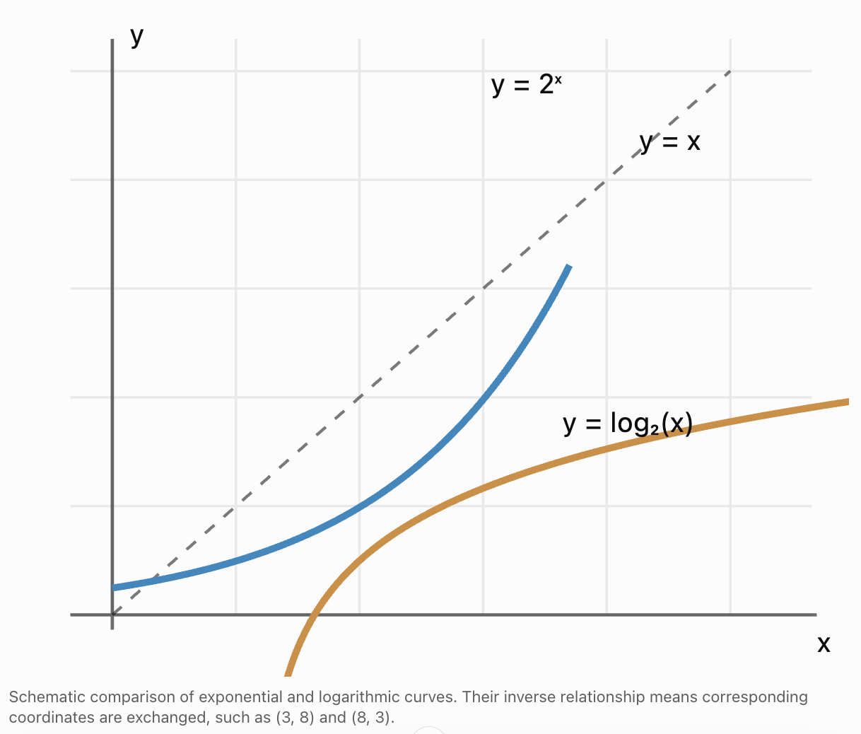
Why Graphs Are Useful
Graphs can help determine:
-
Whether an equation has one or several solutions.
-
Where exponential and logarithmic functions intersect.
-
Whether a solution is reasonable.
-
Which intervals satisfy an inequality.
-
Whether a mathematical model increases or decreases.
Some mixed equations cannot be solved using elementary algebra.
For example:
2ˣ = x + 3
This equation has two real solutions, which can be approximated numerically.
Graphing the functions:
y = 2ˣ
and:
y = x + 3
reveals two intersection points.
Numerical methods give approximately:
x ≈ −2.863 and x ≈ 2.445
In such cases, graphical or numerical methods may be more efficient than attempting to force an algebraic solution.
Evaluating the Reasonableness of Solutions
Finding an answer is only part of solving a mathematical problem.
A complete solution should also consider whether the result makes sense.
Questions to Ask
-
Does the solution satisfy the original equation?
-
Is the value within the allowed domain?
-
Does the sign of the answer make sense?
-
Is the magnitude reasonable?
-
Does the solution agree with an estimate?
-
Are the units correct?
-
Does the result fit the real-world context?
-
Has rounding affected the answer?
-
Does the model have limitations?
Example: Estimating Before Calculating
Solve:
2ˣ = 20
We know:
2⁴ = 16
2⁵ = 32
Therefore:
4 < x < 5
Using logarithms:
x = ln(20)/ln(2)
x ≈ 4.322
This agrees with the estimate.
If the calculator produced x = 43.22, the result would clearly be unreasonable.
Verifying Exact and Approximate Solutions
Exact Solutions
For:
3ˣ = 81
the solution is:
x = 4
Verification:
3⁴ = 81
Approximate Solutions
For:
5ˣ = 17
the exact solution is:
x = ln(17)/ln(5)
Approximately:
x ≈ 1.760
Substituting a rounded value gives an approximate result.
The most accurate verification uses the unrounded logarithmic expression.
Checking Domain Restrictions
Consider:
log₂(x − 3) = 2
Solving gives:
x − 3 = 4
x = 7
The domain requires x > 3.
Since 7 > 3, the solution is valid.
By contrast, any proposed value x ≤ 3 must be rejected before evaluating the logarithm.
Practical Application: Compound Interest
Exponential models describe how investments grow, while logarithms determine the time required to reach a target.
The compound interest formula is:
A = P(1 + r/n)^(nt)
where:
-
A is the final amount.
-
P is the initial investment.
-
r is the annual interest rate.
-
n is the number of compounding periods per year.
-
t is time in years.
Worked Example
An investment of $8000 earns 4.5% annual interest, compounded monthly.
How long will it take to reach $12000?
Step 1: Write the Equation
12000 = 8000(1 + 0.045/12)^(12t)
Step 2: Simplify
1.5 = 1.00375^(12t)
Step 3: Take Natural Logarithms
ln(1.5) = 12t ln(1.00375)
Step 4: Solve
t = ln(1.5)/[12ln(1.00375)]
Step 5: Calculate
t ≈ 9.03 years
Step 6: Evaluate Reasonableness
The investment needs to increase by 50%.
At an annual interest rate of approximately 4.5%, a time of about nine years is reasonable.
Interpretation
The model reaches $12000 after approximately 9.03 years.
Because interest is credited monthly, the account first reaches or exceeds the target after 109 complete months.

Practical Application: Population Growth
Suppose a population grows according to:
P(t) = 1500e^(0.06t)
where t is measured in years.
Worked Example
When will the population exceed 4000?
Step 1: Write the Inequality
1500e^(0.06t) > 4000
Step 2: Divide
e^(0.06t) > 8/3
Step 3: Take Natural Logarithms
0.06t > ln(8/3)
Step 4: Solve
t > ln(8/3)/0.06
Step 5: Calculate
t > 16.35 years
Interpretation
The model predicts that the population exceeds 4000 after approximately 16.35 years.
Reasonableness Check
The initial population is 1500.
The target population is more than twice as large.
At a continuous growth rate of 6%, a time of approximately 16 years is plausible.
However, real populations may not continue growing exponentially indefinitely.
Practical Application: Radioactive Decay
Radioactive decay can be modelled using:
N(t) = N₀e^(−λt)
where:
-
N(t) is the amount remaining.
-
N₀ is the initial amount.
-
λ is the decay constant.
-
t is elapsed time.
Worked Example
A radioactive sample begins with 500 g.
Its decay constant is 0.08 per year.
When will the sample fall below 100 g?
Step 1: Write the Inequality
500e^(−0.08t) < 100
Step 2: Divide
e^(−0.08t) < 0.2
Step 3: Take Natural Logarithms
−0.08t < ln(0.2)
Step 4: Divide by a Negative Number
Reverse the inequality:
t > ln(0.2)/(−0.08)
Step 5: Calculate
t > 20.12 years
Interpretation
The sample falls below 100 g after approximately 20.12 years.
Reasonableness Check
The amount decreases to one-fifth of its initial mass.
A decay constant of 0.08 per year gives a half-life of:
t₁/₂ = ln(2)/0.08
t₁/₂ ≈ 8.66 years
After two half-lives, the amount is one-quarter of the original mass.
Therefore, reaching one-fifth should take slightly longer than two half-lives.
The calculated result is reasonable.


Practical Application: Bacterial Growth
A bacterial population doubles every 3 hours.
The model is:
N(t) = 400 × 2^(t/3)
Worked Example
When will the population reach 10000 bacteria?
Step 1: Write the Equation
10000 = 400 × 2^(t/3)
Step 2: Divide
25 = 2^(t/3)
Step 3: Take Logarithms
ln(25) = (t/3)ln(2)
Step 4: Solve
t = 3ln(25)/ln(2)
Step 5: Calculate
t ≈ 13.93 hours
Reasonableness Check
After four doubling periods, or 12 hours:
N = 400 × 2⁴ = 6400
After five doubling periods, or 15 hours:
N = 400 × 2⁵ = 12800
Therefore, reaching 10000 between 12 and 15 hours is reasonable.
The calculated time of 13.93 hours fits this interval.
Practical Application: pH and Hydrogen-Ion Activity
The pH scale uses a logarithmic relationship:
pH = −log₁₀(a_H⁺)
where a_H⁺ is dimensionless hydrogen-ion activity.
Worked Example
A solution has pH 3.5.
Another solution has pH 5.0.
Compare their hydrogen-ion activities.
Step 1: Use the pH Difference
ΔpH = 5.0 − 3.5
ΔpH = 1.5
Step 2: Calculate the Ratio
Activity ratio = 10^1.5
Step 3: Evaluate
Activity ratio ≈ 31.6
Interpretation
The solution with pH 3.5 has approximately 31.6 times the hydrogen-ion activity of the solution with pH 5.0.
Reasonableness Check
A one-unit pH difference corresponds to a factor of 10.
A two-unit difference corresponds to a factor of 100.
Therefore, a 1.5-unit difference should produce a factor between 10 and 100.
The calculated ratio is reasonable.

Communicating Complete Mathematical Reasoning
A correct numerical answer is not always a complete mathematical solution.
Clear mathematical communication should show how the result was obtained and why it is valid.
A Strong Mathematical Solution Includes
-
A clear statement of the problem.
-
The relevant formula or mathematical principle.
-
Any domain restrictions.
-
Correct substitutions.
-
Logical algebraic steps.
-
Accurate calculations.
-
Verification.
-
Appropriate units.
-
A concluding interpretation.
Example of an Incomplete Solution
Problem:
Solve 3ˣ = 20.
Incomplete answer:
x = 2.727
Although the numerical value is correct, the method is not explained.
Example of a Complete Solution
We are given:
3ˣ = 20
Take natural logarithms:
ln(3ˣ) = ln(20)
Apply the power rule:
xln(3) = ln(20)
Divide by ln(3):
x = ln(20)/ln(3)
Calculate:
x ≈ 2.727
Verification:
3² ≈ 9
3³ = 27
Since 20 lies between 9 and 27, the solution should lie between 2 and 3.
The calculated value is reasonable.
Final Statement
The solution is x = ln(20)/ln(3) ≈ 2.727.
This explanation demonstrates the mathematical reasoning rather than simply reporting the answer.
A General Problem-Solving Strategy
For mixed exponential and logarithmic problems, the following procedure is useful.
Identify the Structure
Determine whether the problem contains:
-
An unknown exponent.
-
An unknown logarithmic argument.
-
Multiple exponential terms.
-
Multiple logarithmic terms.
-
A repeated expression.
-
An inequality.
-
A real-world growth or decay model.
Select an Efficient Method
Choose from:
-
Common bases.
-
Exponent laws.
-
Logarithmic properties.
-
Inverse-function identities.
-
Change of base.
-
Substitution.
-
Factoring.
-
Quadratic formula.
-
Graphical methods.
-
Numerical methods.
Identify Restrictions
Check:
-
Logarithmic arguments must be positive.
-
Exponential expressions with positive bases are positive.
-
Denominators cannot equal zero.
-
Square-root expressions must satisfy real-domain restrictions.
-
Practical quantities may require nonnegative values.
Solve Carefully
Show each algebraic transformation.
Avoid unnecessary rounding.
Verify
Substitute the solution into the original equation or inequality.
Reject invalid candidates.
Evaluate Reasonableness
Estimate expected values and compare with the result.
Communicate the Conclusion
Include units, appropriate precision, and an interpretation.
Common Mistakes
Using logarithms when common bases would be simpler
Always check whether a direct exponent comparison is possible.
Forgetting inverse-function identities
Expressions such as ln(eˣ) can be simplified immediately.
Confusing exponential and logarithmic forms
Remember that aˣ = b is equivalent to logₐ(b) = x.
Applying logarithmic rules incorrectly
For example:
log(a + b) is not generally equal to log(a) + log(b).
Ignoring domain restrictions
Every real logarithmic argument must be positive.
Accepting extraneous solutions
Candidate solutions must satisfy the original equation.
Forgetting positivity after substitution
If u = 2ˣ, then u > 0.
Equating exponents with different bases
Common bases must be established first.
Reversing inequalities incorrectly
An inequality reverses when multiplying or dividing by a negative number.
Rounding too early
Keep exact logarithmic expressions until the final calculation.
Failing to verify solutions
A transformed equation may admit invalid candidates.
Ignoring practical constraints
Real-world models may require nonnegative time or discrete compounding intervals.
Providing an answer without mathematical reasoning
A complete solution should show the method and explain the conclusion.
Failing to evaluate reasonableness
Estimation is a useful way to detect errors.
Key Terms
-
Exponential Function: A function in which the variable appears in an exponent.
-
Logarithmic Function: The inverse of an exponential function.
-
Inverse Function: A function that reverses another function's operation.
-
Exponential Equation: An equation containing an unknown exponent.
-
Logarithmic Equation: An equation containing an unknown variable inside a logarithm.
-
Exponential Inequality: An inequality involving exponential expressions.
-
Logarithmic Inequality: An inequality involving logarithmic expressions.
-
Base: The number raised to a power or used as the base of a logarithm.
-
Exponent: The power to which a base is raised.
-
Argument: The expression inside a logarithm.
-
Common Base: A shared base used to simplify exponential expressions.
-
Natural Logarithm: A logarithm with base e.
-
Common Logarithm: A logarithm with base 10.
-
Change-of-Base Formula: A formula that expresses a logarithm using another base.
-
Product Rule: A logarithmic rule converting multiplication into addition.
-
Quotient Rule: A logarithmic rule converting division into subtraction.
-
Power Rule: A logarithmic rule converting an exponent into a multiplier.
-
Domain: The set of allowable input values.
-
Domain Restriction: A condition limiting valid values of a variable.
-
Extraneous Solution: A candidate solution that does not satisfy the original equation.
-
Substitution: Replacing an expression with a simpler variable.
-
Factorisation: Rewriting an expression as a product of factors.
-
Quadratic Equation: An equation whose highest variable power is 2.
-
Quadratic Formula: A formula used to solve quadratic equations.
-
Graphical Solution: A solution found by examining graphs.
-
Numerical Method: A computational technique used to approximate solutions.
-
Verification: Checking a proposed solution in the original problem.
-
Reasonableness Check: An evaluation of whether a result makes mathematical and practical sense.
-
Exact Solution: A solution expressed without numerical rounding.
-
Approximate Solution: A numerical estimate of an exact value.
-
Exponential Growth: Growth by a constant multiplicative factor over equal intervals.
-
Exponential Decay: Decrease by a constant multiplicative factor over equal intervals.
-
Compound Interest: Interest calculated on an initial principal and accumulated interest.
-
Decay Constant: A parameter describing continuous exponential decay.
-
Half-Life: The time required for a decaying quantity to decrease to half its original amount.
-
Threshold: A boundary value used to determine whether a condition has been reached.
-
Mathematical Model: A mathematical representation of a real-world process.
Key Takeaways
-
Exponential and logarithmic functions are inverse functions.
-
Exponential equations can often be solved using common bases or logarithms.
-
Logarithmic equations can often be solved by converting to exponential form.
-
Inverse-function identities simplify many mixed expressions.
-
Logarithmic properties help combine multiple logarithmic terms.
-
Exponent laws help simplify exponential expressions before solving.
-
Substitution can transform complicated equations into quadratic equations.
-
Factoring and the quadratic formula are useful for solving transformed equations.
-
Domain restrictions must be preserved throughout logarithmic calculations.
-
Exponential expressions with positive bases are always positive.
-
Extraneous solutions must be identified and rejected.
-
Mixed inequalities require careful attention to inequality directions.
-
Graphical methods can help identify the number and approximate locations of solutions.
-
Numerical methods are useful when exact algebraic solutions are impractical.
-
Choosing an efficient method is an important mathematical skill.
-
Complete solutions should include logical algebraic steps and appropriate explanations.
-
Verification ensures that calculated answers satisfy the original problem.
-
Reasonableness checks help identify errors and evaluate mathematical results.
-
Exact expressions should be retained until numerical approximations are required.
-
Exponential and logarithmic models are widely used in finance, biology, chemistry, physics, and environmental science.
-
Practical solutions should include correct units and consideration of model limitations.
-
Successful mixed problem solving requires selecting appropriate techniques, combining them logically, and evaluating the validity and meaning of the final answer.
Check Your Understanding
Recall and Understanding
-
Explain how exponential and logarithmic functions are related.
-
Describe when using common bases is more efficient than using logarithms.
-
Explain why logarithmic domain restrictions must be checked.
-
Describe how substitution can simplify equations containing repeated exponential or logarithmic expressions.
-
Explain why estimating a solution before calculating can be useful.
Application
-
Solve 3^(2x−1) = 50, giving the answer to three decimal places.
-
Solve log₄(3x + 1) = 3.
-
Simplify e^[ln(2x + 5)] and state its domain.
-
Solve 2^(2x) − 5(2ˣ) + 6 = 0.
-
Solve log₂(x) + log₂(x − 4) = 5, checking for extraneous solutions.
Analysis and Challenge
-
Solve [ln(x)]² − 4ln(x) + 3 = 0, giving exact and approximate answers.
-
Solve log₃(x + 2) + log₃(x − 1) = log₃(4x + 4), checking all domain restrictions.
-
Solve 4^(x+1) > 30 using logarithms and express the solution in interval notation.
-
An investment of $7500 earns 5.2% annual interest, compounded monthly. Determine how long it takes to reach $12000 and explain how the answer can be checked for reasonableness.
-
A radioactive substance follows N(t) = 600e^(−0.075t). Determine when its mass falls below 150 g. Show all steps, verify the result, and interpret the answer.
Final Summary
Mixed exponential and logarithmic problems require a flexible approach to mathematical problem solving.
The most important skill is recognising the structure of an equation or inequality and selecting an efficient method.
Common bases, logarithmic properties, inverse-function identities, substitution, factoring, and numerical methods all provide useful techniques.
More advanced problems may require several methods to be combined in a logical sequence.
Domain restrictions and verification are essential, especially when logarithmic expressions or transformed quadratic equations are involved.
Reasonableness checks help determine whether a mathematical result is consistent with expected values and real-world conditions.
Exponential and logarithmic techniques are particularly important in finance, population modelling, radioactive decay, chemistry, and other scientific applications.
The central principle is that effective mathematical problem solving involves more than obtaining an answer: it requires choosing appropriate methods, communicating complete reasoning, verifying solutions, and evaluating whether the results make sense.