Probability Models

Introduction to Probability Models

Probability models help us describe, analyse, and predict situations involving uncertainty.

Many events cannot be predicted with certainty, but mathematical models can help us estimate how likely different outcomes are.

For example:

• What is the probability that a student passes an examination?

• How likely is a machine to produce a defective component?

• What is the probability of rain tomorrow?

• How many customers might arrive at a shop during an hour?

• How likely is a medical test to produce a correct result?

• What is the probability that a project finishes before its deadline?

A probability model is a mathematical representation of a random situation. It identifies possible outcomes and assigns probabilities to those outcomes.

Probability models can be simple, such as rolling a fair die, or complex, such as predicting weather patterns or modelling the reliability of engineering systems.

Constructing useful probability models requires more than selecting a formula. We must identify possible outcomes, evaluate assumptions, select appropriate distributions, calculate probabilities, and interpret the results.

What Is a Probability Model?

A probability model describes the possible outcomes of a random experiment and how probability is distributed among those outcomes.

A complete model generally includes:

• A clearly defined random experiment or situation.

• A sample space containing possible outcomes.

• Events or random variables of interest.

• Probabilities assigned to outcomes or ranges of values.

• Assumptions describing how the system behaves.

Example: Rolling a Fair Die

Consider rolling one fair six-sided die.

The sample space is:

S = 6

Each outcome has probability:

P(X = x) = 1/6

for x = 1, 2, 3, 4, 5, 6.

The probabilities add to:

6 × 1/6 = 1

This is a valid probability model.

Important Principle

A probability model must satisfy two fundamental requirements:

Every probability must be between 0 and 1.

0 ≤ P(E) ≤ 1

The probabilities of all mutually exclusive, exhaustive outcomes must add to 1.

Total probability = 1

These requirements apply to all valid probability models.

Constructing a Probability Model

Constructing a probability model involves several steps.

Identify the Random Experiment

Determine what situation is being investigated.

For example:

A factory selects a manufactured component and checks whether it is defective.

Define the Possible Outcomes

The outcomes might be:

• Defective

• Non-defective

These outcomes are mutually exclusive and exhaustive.

Assign Probabilities

Suppose historical data indicate that 4% of components are defective.

Then:

P(defective) = 0.04

P(non-defective) = 0.96

Check the Probabilities

0.04 + 0.96 = 1

The model is valid.

State the Assumptions

The model assumes:

• The defect rate remains approximately constant.

• The selected component is representative of the production process.

• Defective and non-defective are the only possible classifications.

• The historical defect rate is appropriate for current production.

These assumptions are essential for interpreting the results.

Types of Probability Models

Probability models can be classified in several ways.

Discrete Probability Models

A discrete probability model describes a random variable with a finite or countably infinite set of possible values.

Examples include:

• Number of defective products.

• Number of customers arriving.

• Number of goals scored.

• Number of successful free throws.

Continuous Probability Models

A continuous probability model describes a random variable that can take any real value within an interval or collection of intervals.

Examples include:

• Height.

• Mass.

• Time.

• Temperature.

• Distance.

Theoretical Models

A theoretical model assigns probabilities using mathematical reasoning and assumptions.

For example:

P(rolling a 6 on a fair die) = 1/6

Empirical Models

An empirical model estimates probabilities using observed data.

For example, if a machine produces 25 defective components out of 1,000:

Estimated P(defective) = 25/1000

= 0.025

Simulation Models

A simulation model uses repeated random experiments to estimate probabilities.

For example, a computer might simulate 100,000 dice rolls to estimate the probability of obtaining a particular total.

Common Probability Distributions

Different probability distributions are appropriate for different situations.

Selecting the correct distribution depends on the characteristics of the random variable and the assumptions of the model.

Constructing a Discrete Probability Distribution

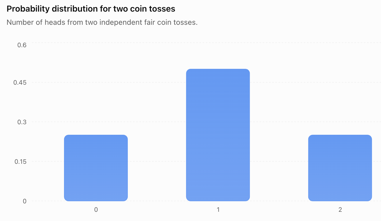
Suppose a game involves tossing two fair coins.

Let X represent the number of heads.

The possible outcomes are:

HH, HT, TH, TT

Step 1: Identify the Values of X

Possible values:

X = 0, 1, 2

Step 2: Count the Outcomes

• X = 0 occurs for TT.

• X = 1 occurs for HT and TH.

• X = 2 occurs for HH.

Step 3: Assign Probabilities

Step 4: Verify the Model

P(X = 0) + P(X = 1) + P(X = 2)

= 1/4 + 2/4 + 1/4

= 1

The model is valid.

Expected Value of a Probability Model

The expected value describes the long-run average outcome of a random variable.

For a discrete random variable:

E(X) = Σ[x × P(X = x)]

The symbol Σ means to add the terms for all possible values of X.

Worked Example: Number of Heads

Using the previous model:

Add:

E(X) = 0 + 0.50 + 0.50

E(X) = 1

The expected number of heads in two fair coin tosses is one.

This does not mean every experiment produces exactly one head.

It describes the average result over many repetitions.

Evaluating Model Assumptions

Every probability model relies on assumptions.

An assumption is a condition accepted as true for the purpose of constructing or using a model.

Assumptions simplify complicated situations and make mathematical analysis possible.

However, unrealistic assumptions can lead to misleading predictions.

Common Probability Assumptions

Independence

One event does not affect the probability of another.

Constant Probability

The probability of an event remains unchanged across trials.

Equal Likelihood

All outcomes have the same probability.

Random Sampling

Observations are selected using an appropriate random process.

Stable Conditions

The system behaves consistently over the period being modelled.

Appropriate Distribution

The selected probability distribution reasonably represents the data.

Example: Basketball Free Throws

Suppose a basketball player has a 75% probability of making a free throw.

A binomial model might assume:

• Each shot has two outcomes: success or failure.

• The number of shots is fixed.

• Each shot is independent.

• The probability of success remains 0.75.

In reality, performance may change because of fatigue, pressure, or confidence.

The binomial model may still be useful, but its assumptions should be considered.

Model Assumptions and Accuracy

A probability model can be mathematically correct while providing inaccurate predictions.

For example, suppose a factory's defect rate increases because a machine is wearing out.

A model assuming a constant 2% defect rate may underestimate future defects.

The calculations could be performed correctly, but the model would no longer describe the actual production process accurately.

Questions for Evaluating a Model

• Are the possible outcomes correctly identified?

• Are probabilities based on reliable information?

• Are the events independent?

• Does the probability remain constant?

• Is the sample representative?

• Does the selected distribution match the observed data?

• Are important variables missing?

• Do predictions agree with observations?

A useful model should be both mathematically valid and appropriate for the situation.

Comparing Competing Probability Models

Sometimes several probability models could describe the same situation.

We must determine which model is most appropriate.

Example: Customer Arrivals

Suppose a shop receives customers throughout the day.

We want to model the number of arrivals during a 10-minute interval.

Possible models include:

Binomial Model

This may be appropriate if there is a fixed number of potential customers, each independently deciding whether to arrive during the interval with the same probability.

Poisson Model

This may be appropriate if customers arrive independently at an approximately constant average rate.

Empirical Model

This uses observed customer counts without assuming a particular theoretical distribution.

Comparing the Models

The best model depends on the situation and available evidence.

Worked Example: Choosing a Probability Model

A call centre receives an average of four calls per minute.

We want to calculate the probability of receiving exactly six calls in one minute.

A Poisson distribution may be appropriate if calls arrive independently at a constant average rate.

Let:

X = number of calls per minute

λ = 4

Then:

X ~ Poisson(4)

The Poisson probability formula is:

P(X = k) = e^(−λ) × λᵏ/k!

Substitute:

P(X = 6) = e^(−4) × 4⁶/6!

= e^(−4) × 4096/720

P(X = 6) ≈ 0.1042

There is approximately a 10.42% probability of receiving exactly six calls in one minute under this model.

Evaluating the Model

The Poisson model may be unsuitable if:

• Calls arrive in clusters.

• The call rate changes significantly during the interval.

• One call causes additional calls.

• The arrival process is not independent.

The probability is conditional on the model assumptions being reasonable.

Comparing Theoretical Models with Observed Data

A useful way to evaluate a model is to compare its predictions with actual observations.

Suppose a model predicts the following probabilities for the number of customers arriving during a short interval.

The observed frequencies are reasonably close to the predicted frequencies.

However, differences remain because of random variation.

Evaluating the Fit

A model can be evaluated by considering:

• Differences between predicted and observed frequencies.

• Patterns in the errors.

• Whether some outcomes occur more often than expected.

• Whether the model remains accurate over time.

Formal statistical methods, such as goodness-of-fit tests, can provide additional evidence about model suitability.

Model Error and Uncertainty

Probability models involve different sources of uncertainty.

Random Variation

Even when a model is correct, actual outcomes vary randomly.

For example, a fair coin may produce seven heads in ten tosses.

Sampling Error

Probabilities estimated from samples may differ from population probabilities.

Measurement Error

Observations may contain inaccuracies.

Model Error

The mathematical model may fail to represent important features of the real system.

Parameter Uncertainty

The values used in the model, such as a success probability or event rate, may be estimated imperfectly.

Important Distinction

Increasing the sample size generally reduces sampling error.

However, it does not automatically correct an inappropriate probability model.

Solving Applied Probability Problems

Many practical probability problems involve several events or conditions.

The most important step is choosing an appropriate model.

Worked Example: Manufacturing Defects

A factory produces components with a 3% probability of being defective.

Suppose ten components are selected independently.

Find the probability that exactly two are defective.

Step 1: Select the Model

The number of defects follows a binomial distribution under the stated assumptions.

X ~ B(10, 0.03)

Step 2: Apply the Formula

P(X = k) = C(n,k) × pᵏ × (1 − p)^(n−k)

Substitute:

P(X = 2) = C(10,2) × 0.03² × 0.97⁸

Since:

C(10,2) = 45

P(X = 2) = 45 × 0.0009 × 0.97⁸

P(X = 2) ≈ 0.0317

There is approximately a 3.17% probability that exactly two of the ten components are defective.

Interpretation

This probability is valid if the defect probability remains constant and the selected components can reasonably be treated as independent.

Worked Example: Continuous Probability Model

Suppose a bus arrives at a uniformly random time between 0 and 12 minutes after a passenger reaches the bus stop.

Let:

X = waiting time

X ~ U(0, 12)

Find the probability that the passenger waits between 3 and 7 minutes.

Step 1: Determine the Interval Lengths

Total interval:

12 − 0 = 12 minutes

Favourable interval:

7 − 3 = 4 minutes

Step 2: Calculate the Probability

P(3 ≤ X ≤ 7) = 4/12

P(3 ≤ X ≤ 7) = 1/3 ≈ 0.3333

There is approximately a 33.33% probability that the passenger waits between three and seven minutes.

Model Evaluation

This assumes that arrival time is uniformly distributed across the interval.

If buses are more likely to arrive near particular times, the uniform model would be inappropriate.

Worked Example: Conditional Probability Model

Suppose a factory uses two machines.

Machine A produces 60% of components.

Machine B produces 40%.

The defect rates are:

• Machine A: 2%.

• Machine B: 5%.

Find the probability that a randomly selected component is defective.

Step 1: Define Events

A = component produced by Machine A

B = component produced by Machine B

D = component is defective

Step 2: Apply the Law of Total Probability

P(D) = P(D | A)P(A) + P(D | B)P(B)

Substitute:

P(D) = 0.02 × 0.60 + 0.05 × 0.40

= 0.012 + 0.020

P(D) = 0.032

There is a 3.2% probability that a randomly selected component is defective.

Why This Model Is Appropriate

The calculation accounts for both machines and their different production proportions.

Using a simple average of the two defect rates would be inappropriate because the machines produce different proportions of the total output.

Worked Example: Comparing Two Models

Suppose a company wants to estimate the number of defective products in a shipment.

Two possible models are proposed.

Model A: Binomial

Each product independently has a 4% probability of being defective.

Model B: Poisson

The number of defects is modelled using a Poisson distribution with mean 4 per 100 products.

For a shipment of 100 products:

Model A:

X ~ B(100, 0.04)

Model B:

X ~ Poisson(4)

Probability of No Defects

For the binomial model:

P(X = 0) = 0.96¹⁰⁰

≈ 0.0169

For the Poisson model:

P(X = 0) = e^(−4)

≈ 0.0183

The results are similar.

Interpretation

The Poisson model can approximate a binomial model when the number of trials is large and the success probability is small.

However, the approximation is not exact.

The binomial model may be preferable when the fixed number of trials and individual defect probability are known.

Using Simulation to Evaluate Models

Simulation can help evaluate a probability model by generating outcomes and comparing them with theoretical predictions.

For example, suppose a binomial model predicts:

P(success) = 0.6

A simulation can generate thousands of independent trials with a 60% success probability.

The resulting success proportion should generally be close to 0.6 when enough trials are performed.

Simulation Procedure

1. Define the probability model.

2. Generate random outcomes according to the model.

3. Repeat the experiment many times.

4. Calculate simulated probabilities.

5. Compare simulated results with theoretical predictions.

6. Investigate any substantial differences.

Important Limitation

A simulation that uses the same assumptions as the theoretical model mainly checks the calculation or implementation.

It does not prove that the model accurately describes the real world.

Real observations are needed to evaluate the model's practical validity.

Sensitivity Analysis

Sensitivity analysis investigates how changes in model assumptions or parameters affect the results.

Suppose a factory estimates a 3% defect probability.

However, the true defect probability may be between 2% and 5%.

For ten independent components, the probability of at least one defect is:

P(at least one defect) = 1 − (1 − p)¹⁰

Calculate this probability for different values of p.

The probability of at least one defect changes substantially as the assumed defect rate increases.

Interpretation

The model's predictions are sensitive to the value of p.

This means that accurately estimating the defect rate is important.

Sensitivity analysis helps identify which assumptions have the greatest influence on model results.

Probability Models in Science

Probability models are widely used in scientific investigations.

Genetics

Probability can describe the likelihood of inheriting particular genetic combinations under specified inheritance models.

Ecology

Models can estimate population changes, species survival, or movement between habitats.

Chemistry

Probability models can describe random molecular behaviour and certain reaction processes.

Physics

Probability is important in radioactive decay, statistical mechanics, and quantum phenomena.

Environmental Science

Models can estimate rainfall, flooding, pollution exposure, and other uncertain environmental events.

Probability Models in Business and Engineering

Insurance

Insurance companies use probability models to estimate the frequency and cost of claims.

Manufacturing

Factories model defect rates, equipment failures, and product reliability.

Transportation

Probability models can estimate travel times, traffic delays, and vehicle arrivals.

Finance

Models can estimate uncertain returns, losses, and financial risks.

Project Management

Probability models can estimate completion times and the likelihood of meeting deadlines.

These applications often involve several uncertain variables, making model selection and evaluation especially important.

Communicating Probability Reasoning

A probability calculation is most useful when it is explained clearly.

A complete solution should communicate:

• What is being investigated.

• Which events or random variables are involved.

• Which probability model is being used.

• Why the model is appropriate.

• Which assumptions are required.

• How the calculation is performed.

• What the result means in context.

• What limitations may affect the conclusion.

Example of a Clear Probability Explanation

A factory produces components with a 5% probability of being defective.

Assuming ten components are selected independently and the defect probability remains constant, the number of defective components follows a binomial distribution.

The probability that all ten components are non-defective is:

P(X = 0) = 0.95¹⁰

≈ 0.5987

Therefore, there is approximately a 59.87% probability that none of the ten components is defective.

This result depends on the assumptions of independence and constant defect probability.

Why This Is Effective

The explanation identifies:

• The situation.

• The mathematical model.

• The assumptions.

• The calculation.

• The interpretation.

It communicates both the numerical result and the reasoning behind it.

Evaluating Competing Models

When several models are available, compare them systematically.

Model Selection Criteria

Accuracy

How closely does the model match observed data?

Simplicity

Is the model unnecessarily complicated?

Assumptions

Are the assumptions realistic?

Interpretability

Can the model's predictions be explained clearly?

Data Requirements

Is enough reliable information available to estimate the parameters?

Predictive Performance

Does the model make accurate predictions on new observations?

Practical Usefulness

Does the model provide information that helps answer the original question?

The Balance Between Simplicity and Accuracy

A simple model may be easier to understand and apply.

A more complex model may capture additional details.

However, complexity does not automatically improve predictions.

The best model is one that represents the important features of the situation without unnecessary complication.

Common Mistakes

Selecting a distribution without checking its assumptions

Different distributions require different conditions.

Assuming all outcomes are equally likely

Many real-world outcomes have different probabilities.

Ignoring dependence between events

Dependent events require conditional probability calculations or other suitable models.

Confusing discrete and continuous variables

Counts and measurements often require different probability distributions.

Using a simple average when a weighted average is required

Groups contributing different proportions must be weighted appropriately.

Assuming a mathematically valid model is realistic

A model can satisfy probability rules while failing to represent real-world behaviour.

Ignoring sampling error

Probabilities estimated from samples contain uncertainty.

Confusing simulation accuracy with model validity

A simulation may reproduce the model accurately even when the model is inappropriate.

Comparing models using only one prediction

Models should be evaluated across relevant outcomes and observations.

Reporting probabilities without context

A numerical answer should be interpreted in terms of the original problem.

Failing to state assumptions

Assumptions are essential for understanding when a probability calculation is valid.

Key Terms

• Probability Model: A mathematical representation of possible outcomes and their probabilities.

• Random Experiment: A process whose outcome is uncertain.

• Sample Space: The set of all possible outcomes of an experiment.

• Event: A collection of outcomes within a sample space.

• Random Variable: A numerical variable whose value depends on a random outcome.

• Discrete Random Variable: A random variable with a finite or countably infinite set of possible values.

• Continuous Random Variable: A random variable that can take any real value within an interval or collection of intervals.

• Probability Distribution: A description of how probability is assigned to possible values.

• Theoretical Probability: A probability calculated using mathematical assumptions.

• Empirical Probability: A probability estimated using observed data.

• Simulation: A process that imitates uncertain outcomes using a mathematical or computational model.

• Bernoulli Distribution: A probability model for a single success-or-failure trial.

• Binomial Distribution: A probability model for the number of successes in a fixed number of independent trials.

• Geometric Distribution: A probability model for the number of trials until the first success.

• Poisson Distribution: A probability model for counts of events occurring at a constant average rate under specified assumptions.

• Uniform Distribution: A distribution with equally likely discrete outcomes or constant density over a continuous interval.

• Normal Distribution: A symmetrical, bell-shaped continuous probability distribution.

• Exponential Distribution: A continuous distribution commonly used to model waiting times in a Poisson process.

• Expected Value: The long-run average outcome of a random variable.

• Variance: A measure of how widely values are spread around the mean.

• Model Assumption: A condition accepted when constructing or applying a model.

• Independence: A relationship in which one event does not change the probability of another.

• Conditional Probability: The probability of an event given that another event has occurred.

• Parameter: A numerical value describing a probability distribution.

• Model Error: Error caused by differences between the mathematical model and the real system.

• Sampling Error: Variation caused by estimating quantities from a sample.

• Goodness of Fit: A measure of how closely a model agrees with observed data.

• Sensitivity Analysis: An investigation of how model results change when assumptions or parameters change.

• Predictive Performance: How accurately a model predicts new outcomes.

• Probability Reasoning: The use of mathematical evidence and logical explanations to analyse uncertainty.

Key Takeaways

• Probability models describe uncertain situations using possible outcomes and assigned probabilities.

• A valid probability model assigns probabilities between 0 and 1.

• The probabilities of mutually exclusive, exhaustive outcomes must add to 1.

• Constructing a probability model requires defining the experiment, outcomes, probabilities, and assumptions.

• Discrete probability models describe countable outcomes, while continuous models describe values across intervals.

• Different probability distributions are appropriate for different situations.

• Bernoulli, binomial, geometric, and Poisson distributions are common discrete models.

• Uniform, normal, and exponential distributions are important continuous models.

• Expected value describes the long-run average outcome of a probability model.

• Every probability model depends on assumptions.

• Independence, constant probabilities, random sampling, and distribution shape are common assumptions.

• A mathematically correct model may still produce inaccurate real-world predictions.

• Competing models should be compared using assumptions, accuracy, simplicity, and predictive performance.

• Observed data can be used to evaluate how well a model fits a situation.

• Simulation provides a useful way to investigate complex probability models.

• Sensitivity analysis shows how predictions change when model parameters change.

• Probability models are widely used in science, manufacturing, finance, transportation, and engineering.

• Clear probability reasoning includes the model, assumptions, calculations, interpretation, and limitations.

Check Your Understanding

Recall and Understanding

1. Define a probability model and explain its purpose.

2. State the two fundamental requirements of a valid probability model.

3. Explain the difference between discrete and continuous probability models.

4. Identify three assumptions commonly used in probability modelling.

5. Explain why a mathematically correct model may still produce inaccurate predictions.

Application

6. A fair die is rolled once. Construct a probability model for the outcome and verify that the probabilities add to 1.

7. Two fair coins are tossed. Construct a probability distribution for the number of heads and calculate its expected value.

8. A factory produces components with a 4% probability of being defective. Assuming independence, calculate the probability that exactly one of five components is defective.

9. A call centre receives an average of three calls per minute. Assuming a Poisson model is appropriate, calculate the probability of receiving exactly two calls in one minute.

10. A bus arrives uniformly between 0 and 15 minutes after a passenger begins waiting. Calculate the probability that the waiting time is between 5 and 10 minutes.

Analysis and Challenge

11. A basketball player makes 80% of free throws. Explain the assumptions required to model the number of successes in ten attempts using a binomial distribution.

12. A factory uses two machines. Machine A produces 70% of components with a 2% defect rate, while Machine B produces 30% with a 6% defect rate. Calculate the overall probability that a component is defective.

13. A company is comparing a binomial model and a Poisson model for the number of defects in a shipment. Explain when each model would be appropriate and identify the limitations of the Poisson approximation.

14. A probability model predicts that 10% of products will be defective, but observed data show that 18% are defective. Suggest possible reasons for the difference and explain how the model could be improved.

15. Design a probability model for a real-world situation of your choice. Define the random variable, select an appropriate distribution, state the assumptions, demonstrate one probability calculation, and explain how you would evaluate the model's accuracy.

Final Summary

Probability models provide a structured mathematical approach to understanding and predicting uncertain outcomes.

Constructing a model involves identifying possible outcomes, assigning probabilities, selecting suitable distributions, and stating the assumptions required.

Different models are appropriate for different situations, and no single distribution can describe every random process.

Evaluating probability models requires comparing predictions with observations, examining assumptions, and considering uncertainty and model limitations.

By selecting appropriate models, performing calculations, and communicating reasoning clearly, students can apply probability to practical problems in science, engineering, business, and everyday life.

The most important principle is that a probability model is useful not simply because it produces a numerical answer, but because its assumptions and predictions provide a reasonable representation of the situation being studied.