Advanced Probability
| 站点: | Young Education |
| 课程: | Probability and Combinatorics |
| 图书: | Advanced Probability |
| 打印: | Guest user |
| 日期: | 2026年11月9日 星期一 16:41 |
1. Bayes' Theorem
Learning outcomes
- I can explain Bayes' Theorem.
- I can calculate posterior probabilities.
- I can interpret Bayesian reasoning.
- I can solve diagnostic testing problems.
- I can apply Bayesian thinking to real-world situations.
Bayes' Theorem
Introduction to Bayes' Theorem
In everyday life, we often make decisions using incomplete information. When new evidence becomes available, we may need to reconsider what we previously believed.
For example:
-
A medical test produces a positive result. How likely is it that the patient actually has the condition?
-
A factory inspection identifies a defective product. Which machine most likely produced it?
-
An email is flagged as spam. How likely is it to be unwanted?
-
A weather forecast predicts rain. How should new weather observations change that prediction?
-
A scientific experiment produces unexpected results. How should researchers update their hypotheses?
These situations involve conditional probability and Bayesian reasoning.
Bayes' Theorem is a mathematical rule that allows us to update the probability of an event when new evidence becomes available.
It connects what we believed before observing the evidence with what we should believe after considering it.


Reviewing Conditional Probability
Before studying Bayes' Theorem, it is important to understand conditional probability.
A conditional probability describes the probability of an event occurring when another event is already known to have occurred.
It is written as:
P(A | B)
This is read as:
"The probability of A given B."
For example:
-
A = a student passes an examination.
-
B = the student attended a revision session.
Then:
P(A | B)
represents the probability that a student passes the examination, given that the student attended the revision session.
Conditional Probability Formula
P(A | B) = P(A ∩ B)/P(B)
where:
-
P(A | B) is the probability of A given B.
-
P(A ∩ B) is the probability that both A and B occur.
-
P(B) is the probability of B.
This formula requires P(B) > 0.
Worked Example: Students and Sports
Suppose a school has 100 students.
-
40 students play basketball.
-
30 students play football.
-
15 students play both sports.
Let:
A = student plays basketball
B = student plays football
Find the probability that a student plays basketball, given that the student plays football.
P(A | B) = P(A ∩ B)/P(B)
= (15/100)/(30/100)
= 15/30
P(A | B) = 0.5
There is a 50% probability that a student plays basketball, given that the student plays football.
Why Conditional Probabilities Are Different
One of the most important ideas in Bayesian reasoning is that:
P(A | B) is not generally equal to P(B | A).
For example:
-
P(positive test | disease) describes how often a test correctly identifies people who have a disease.
-
P(disease | positive test) describes how likely a person is to have the disease after receiving a positive result.
These probabilities answer different questions.
A medical test can correctly identify most people with a disease while many positive results still occur among people who do not have the disease.
Understanding this distinction is essential for interpreting diagnostic tests, scientific evidence, and statistical claims.
Understanding Bayes' Theorem
Bayes' Theorem provides a method for reversing conditional probabilities.
The formula is:
P(A | B) = [P(B | A) × P(A)]/P(B)
where:
-
P(A | B) is the probability of A after observing B.
-
P(B | A) is the probability of observing B if A is true.
-
P(A) is the probability of A before observing B.
-
P(B) is the overall probability of observing B.
The formula requires P(B) > 0.
Understanding the Components
Bayes' Theorem can be expressed conceptually as:
Posterior probability = Likelihood × Prior probability / Evidence probability
Each part has a specific meaning.
|
Term |
Meaning |
|---|---|
|
Prior probability |
Initial probability before new evidence |
|
Likelihood |
Probability of observing the evidence if the hypothesis is true |
|
Evidence probability |
Overall probability of observing the evidence |
|
Posterior probability |
Updated probability after considering the evidence |
Bayes' Theorem describes how evidence changes our estimate of a probability.
Prior and Posterior Probabilities
Prior Probability
The prior probability is the probability assigned to an event before considering new evidence.
For example, suppose 5% of manufactured products are defective.
Before inspecting a randomly selected product:
P(defective) = 0.05
This is the prior probability.
Posterior Probability
The posterior probability is the updated probability after considering new evidence.
Suppose an inspection system identifies the product as potentially defective.
We can use Bayes' Theorem to determine the probability that the product is actually defective, given the inspection result.
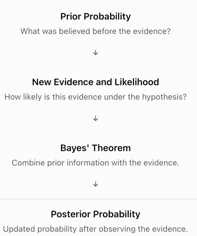
Bayesian Updating
The process can be summarized as:
The Law of Total Probability
Bayes' Theorem often requires calculating the overall probability of the evidence.
Suppose A and not A are the only two possibilities.
Then:
P(B) = P(B | A)P(A) + P(B | not A)P(not A)
This is an application of the Law of Total Probability.
It considers two different ways that event B can occur:
-
B occurs when A is true.
-
B occurs when A is false.
The probabilities of these two mutually exclusive possibilities are added.
Expanded Form of Bayes' Theorem
Substituting the total probability formula gives:
P(A | B) = [P(B | A)P(A)]/[P(B | A)P(A) + P(B | not A)P(not A)]
This form is particularly useful for diagnostic testing problems.
Worked Example: A Simple Bayesian Calculation
Suppose a factory produces electronic components.
-
10% of components are defective.
-
An inspection system flags 90% of defective components.
-
The system also flags 20% of non-defective components.
A component is flagged.
What is the probability that it is actually defective?
Step 1: Define the Events
Let:
D = component is defective
F = component is flagged
We know:
P(D) = 0.10
P(not D) = 0.90
P(F | D) = 0.90
P(F | not D) = 0.20
We want:
P(D | F)
Step 2: Calculate the Overall Probability of Being Flagged
P(F) = P(F | D)P(D) + P(F | not D)P(not D)
= (0.90 × 0.10) + (0.20 × 0.90)
= 0.09 + 0.18
P(F) = 0.27
Step 3: Apply Bayes' Theorem
P(D | F) = [P(F | D)P(D)]/P(F)
= (0.90 × 0.10)/0.27
= 0.09/0.27
P(D | F) ≈ 0.3333
Interpretation
There is approximately a 33.33% probability that a flagged component is actually defective.
Although the inspection system detects 90% of defective components, many flagged components are not defective because non-defective components are much more common.
This demonstrates why the prior probability matters.
Understanding Bayesian Reasoning with Frequency Tables
Bayesian calculations can become easier to understand when probabilities are converted into expected frequencies.
Using the previous example, suppose the factory produces 1,000 components.
Step 1: Determine the Number of Defective Components
10% are defective.
1,000 × 0.10 = 100
Therefore:
-
100 components are defective.
-
900 components are non-defective.
Step 2: Apply the Inspection Results
Of the 100 defective components:
90% are flagged.
100 × 0.90 = 90
Of the 900 non-defective components:
20% are flagged.
900 × 0.20 = 180
Step 3: Construct a Table
|
Actual condition |
Flagged |
Not flagged |
Total |
|---|---|---|---|
|
Defective |
90 |
10 |
100 |
|
Non-defective |
180 |
720 |
900 |
|
Total |
270 |
730 |
1,000 |
Step 4: Calculate the Posterior Probability
Of the 270 flagged components, 90 are actually defective.
P(defective | flagged) = 90/270
P(defective | flagged) = 1/3 ≈ 33.33%
The frequency-table method produces the same result as Bayes' Theorem.

Bayes' Theorem and Diagnostic Testing
One of the most important applications of Bayes' Theorem is interpreting diagnostic tests.
A diagnostic test may be used to identify a medical condition.
However, test results are not always correct.
Two important measures describe test performance.
Sensitivity
Sensitivity is the probability that a test gives a positive result when the condition is present.
Sensitivity = P(positive | condition)
A test with 95% sensitivity correctly identifies 95% of people who have the condition.
Specificity
Specificity is the probability that a test gives a negative result when the condition is absent.
Specificity = P(negative | no condition)
A test with 90% specificity correctly identifies 90% of people who do not have the condition.
False Positive Rate
A false positive occurs when the test gives a positive result even though the condition is absent.
False positive rate = 1 − specificity
False Negative Rate
A false negative occurs when the test gives a negative result even though the condition is present.
False negative rate = 1 − sensitivity
Worked Example: Medical Diagnostic Testing
Suppose a medical condition affects 1% of a population.
A diagnostic test has:
-
Sensitivity = 95%
-
Specificity = 90%
A randomly selected person receives a positive result.
What is the probability that the person actually has the condition?
Step 1: Define the Events
Let:
D = person has the condition
T = positive test result
We know:
P(D) = 0.01
P(not D) = 0.99
P(T | D) = 0.95
Specificity = 0.90
Therefore:
P(T | not D) = 0.10
Step 2: Calculate the Probability of a Positive Result
P(T) = P(T | D)P(D) + P(T | not D)P(not D)
= (0.95 × 0.01) + (0.10 × 0.99)
= 0.0095 + 0.099
P(T) = 0.1085
Step 3: Apply Bayes' Theorem
P(D | T) = [P(T | D)P(D)]/P(T)
= (0.95 × 0.01)/0.1085
= 0.0095/0.1085
P(D | T) ≈ 0.0876
Final Answer
There is approximately an 8.76% probability that a person actually has the condition after receiving a positive result, under the assumptions of this example.
Why Is the Probability So Low?
The condition is rare.
Although the test correctly identifies most people who have the condition, false positives occur among the much larger group of people who do not have it.
This is known as the base-rate effect.
A positive result does not automatically mean that the condition is likely to be present.

Visualizing the Diagnostic Testing Example
Imagine testing 10,000 people.
Since the condition affects 1% of the population:
-
100 people have the condition.
-
9,900 people do not have the condition.
With 95% sensitivity:
-
95 of the 100 people with the condition test positive.
-
5 test negative.
With 90% specificity:
-
990 of the 9,900 people without the condition test positive.
-
8,910 test negative.
|
Actual condition |
Positive test |
Negative test |
Total |
|---|---|---|---|
|
Condition present |
95 |
5 |
100 |
|
Condition absent |
990 |
8,910 |
9,900 |
|
Total |
1,085 |
8,915 |
10,000 |
Of the 1,085 positive results, only 95 are true positives.
Therefore:
P(condition | positive) = 95/1085
≈ 0.0876 = 8.76%
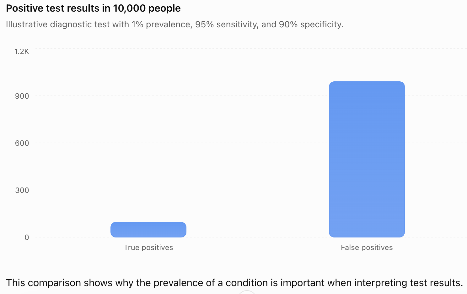
This comparison shows why the prevalence of a condition is important when interpreting test results.
Positive and Negative Predictive Values
Two additional measures are useful in diagnostic testing.
Positive Predictive Value
The positive predictive value (PPV) is the probability that a person has the condition given a positive test result.
PPV = P(condition | positive)
This is the posterior probability calculated using Bayes' Theorem.
Negative Predictive Value
The negative predictive value (NPV) is the probability that a person does not have the condition given a negative test result.
NPV = P(no condition | negative)
Using the previous example:
NPV = 8910/8915
NPV ≈ 0.9994 = 99.94%
Under this example's assumptions, a negative result is very likely to be correct.
Important Distinction
Sensitivity and specificity describe how a test performs among people whose actual condition is known.
Predictive values describe what a positive or negative result means for the person being tested.
Predictive values depend on the prevalence of the condition in the tested population.
How Prior Probability Affects Posterior Probability
Suppose a diagnostic test has:
-
Sensitivity = 95%
-
Specificity = 90%
The posterior probability after a positive result changes depending on how common the condition is.
|
Prevalence |
Probability of condition after positive test |
|---|---|
|
1% |
8.76% |
|
5% |
33.33% |
|
10% |
51.35% |
|
20% |
70.37% |
|
50% |
90.48% |
The test itself has not changed.
Only the prior probability has changed.
This demonstrates a central idea of Bayesian reasoning:
The same evidence can produce different posterior probabilities when the prior probabilities differ.
Probability Trees and Bayes' Theorem
Probability trees provide another way to organize conditional probabilities.
Consider a simplified factory example.
-
20% of products come from Machine A.
-
80% come from Machine B.
-
Machine A produces defective products 10% of the time.
-
Machine B produces defective products 5% of the time.
We want to determine the probability that a defective product came from Machine A.
Step 1: Identify the Branches
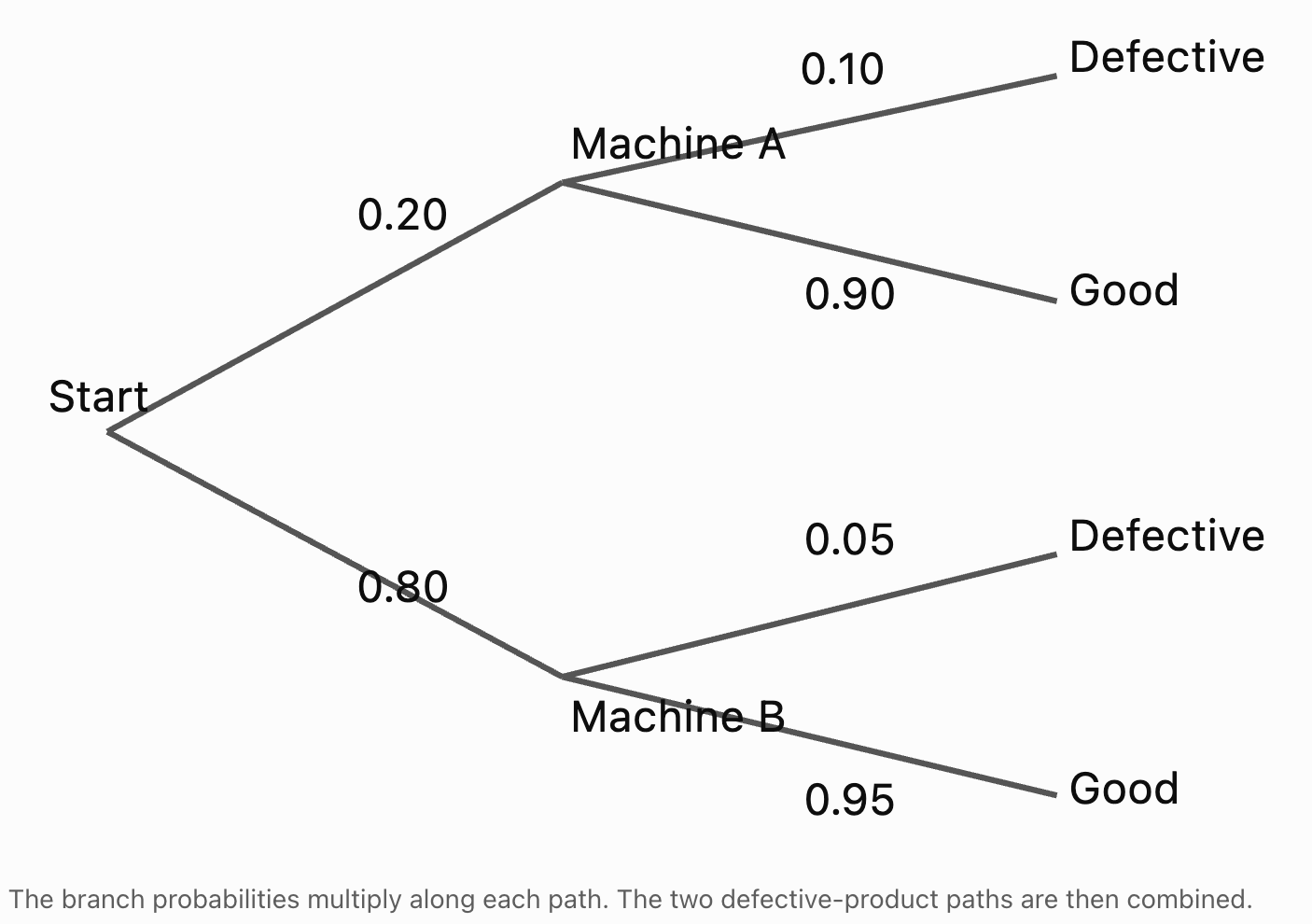
Step 2: Calculate the Probability of a Defective Product from Each Machine
Machine A:
P(A and defective) = 0.20 × 0.10
= 0.02
Machine B:
P(B and defective) = 0.80 × 0.05
= 0.04
Step 3: Calculate the Total Probability of a Defect
P(defective) = 0.02 + 0.04
= 0.06
Step 4: Apply Bayes' Theorem
P(A | defective) = 0.02/0.06
P(A | defective) ≈ 0.3333
There is approximately a 33.33% probability that a defective product came from Machine A.
Although Machine A has a higher defect rate, Machine B produces more products overall.
Bayesian Reasoning in Everyday Life
Bayesian reasoning is not limited to formal probability calculations.
It describes a general process of updating beliefs when new information becomes available.
Weather Forecasting
A meteorologist may initially estimate a 30% probability of rain.
New satellite observations may provide evidence that increases or decreases this estimate.
The updated probability incorporates both the original forecast and the new evidence.
Email Spam Detection
An email system may estimate the probability that a message is spam.
Evidence might include:
-
Certain words or phrases.
-
Suspicious links.
-
Sender characteristics.
-
Previous patterns of unwanted messages.
The system can use probabilistic methods to update its estimate.
Scientific Investigations
Scientists often compare competing explanations for observed results.
As new experimental evidence becomes available, the relative support for different hypotheses may change.
Quality Control
Manufacturers can use inspection results to estimate the probability that a product is defective or that a particular machine caused a problem.


Bayesian Updating with Multiple Pieces of Evidence
Bayesian reasoning can be repeated as new evidence becomes available.
Suppose an initial probability is:
P(A) = 0.20
After observing evidence B, the probability is updated to:
P(A | B) = 0.60
If additional evidence C becomes available, the updated probability can be revised again:
P(A | B and C)
The previous posterior probability becomes part of the information used in the next update.
Sequential Updating
The process is:
Prior → Evidence → Posterior → New Evidence → New Posterior
This is useful in:
-
Medical investigations.
-
Scientific experiments.
-
Machine learning.
-
Weather forecasting.
-
Engineering diagnostics.
Important Limitation
Evidence must be combined carefully.
If two observations are related, treating them as independent can lead to incorrect probabilities.
For example, two medical tests may share the same sources of error.
Bayesian updating must account for such dependencies.
Bayesian Reasoning and Decision-Making
Bayes' Theorem can help people make decisions when information is incomplete.
However, probability alone does not determine the best decision.
Decision-makers must also consider the consequences of different outcomes.
For example, suppose a machine has a 10% probability of malfunctioning.
An inspection provides evidence that increases the estimated probability to 60%.
The company may decide to stop the machine for maintenance.
The decision depends on:
-
The updated probability of malfunction.
-
The cost of maintenance.
-
The cost of a possible failure.
-
Safety considerations.
-
Available alternatives.
Bayesian reasoning provides an improved estimate of uncertainty, while decision analysis considers what action should follow.
The Base-Rate Fallacy
A common error in probability reasoning is ignoring the initial frequency of an event.
This is called the base-rate fallacy.
Example
Suppose a rare condition affects only 1% of a population.
A test correctly identifies 99% of people with the condition.
Someone might conclude that a positive result means there is a 99% probability of having the condition.
This conclusion is not justified.
The probability after a positive result also depends on the false positive rate and the prevalence of the condition.
A highly sensitive test does not automatically have a high positive predictive value.
Avoiding the Base-Rate Fallacy
When interpreting evidence, always ask:
-
How common was the event before the evidence?
-
How likely is the evidence if the event is true?
-
How likely is the same evidence if the event is false?
These questions form the foundation of Bayesian reasoning.
Common Mistakes
Confusing P(A | B) with P(B | A)
Conditional probabilities are not generally interchangeable.
Ignoring the prior probability
Bayes' Theorem requires considering how likely an event was before the evidence.
Confusing sensitivity with positive predictive value
Sensitivity describes test performance among people with the condition. Positive predictive value describes the probability of the condition after a positive result.
Forgetting false positives
Evidence may occur even when the hypothesis is false.
Using the wrong denominator
The denominator in Bayes' Theorem is the overall probability of the observed evidence.
Forgetting the Law of Total Probability
Evidence can often arise through multiple mutually exclusive possibilities.
Assuming a positive test proves a condition is present
A positive result changes probability but does not establish certainty.
Ignoring the base rate
Rare events can remain relatively unlikely even after apparently strong evidence.
Treating dependent evidence as independent
Related observations may contain overlapping information.
Confusing probability with decision-making
An updated probability helps inform a decision, but consequences and costs must also be considered.
Key Terms
-
Bayes' Theorem: A mathematical rule for updating probabilities using new evidence.
-
Conditional Probability: The probability of an event occurring given that another event has occurred.
-
Prior Probability: The probability assigned to a hypothesis before considering new evidence.
-
Posterior Probability: The updated probability of a hypothesis after considering evidence.
-
Likelihood: The probability of observing particular evidence under a specified hypothesis.
-
Evidence Probability: The overall probability of observing the evidence.
-
Bayesian Updating: The process of revising probabilities when new information becomes available.
-
Law of Total Probability: A rule for calculating the probability of an event by combining probabilities across mutually exclusive cases.
-
Hypothesis: A proposed explanation or claim being evaluated.
-
Evidence: Information or observations used to evaluate a hypothesis.
-
Base Rate: The initial frequency or prevalence of an event in a population.
-
Base-Rate Fallacy: The error of ignoring prior probabilities when interpreting evidence.
-
Sensitivity: The probability that a diagnostic test is positive when the condition is present.
-
Specificity: The probability that a diagnostic test is negative when the condition is absent.
-
True Positive: A positive test result for someone who has the condition.
-
False Positive: A positive test result for someone who does not have the condition.
-
True Negative: A negative test result for someone who does not have the condition.
-
False Negative: A negative test result for someone who has the condition.
-
Positive Predictive Value: The probability that a condition is present given a positive test result.
-
Negative Predictive Value: The probability that a condition is absent given a negative test result.
-
Probability Tree: A branching diagram representing possible events and their probabilities.
-
Frequency Table: A table showing counts of outcomes in different categories.
-
Sequential Updating: Repeatedly revising probabilities as additional evidence becomes available.
-
Decision Analysis: The process of comparing possible actions using probabilities and consequences.
Key Takeaways
-
Bayes' Theorem allows probabilities to be updated when new evidence becomes available.
-
Conditional probability describes the likelihood of an event given that another event has occurred.
-
P(A | B) is not generally equal to P(B | A).
-
Bayes' Theorem connects prior probability, likelihood, evidence probability, and posterior probability.
-
The prior probability represents what was known before observing new evidence.
-
The posterior probability represents the updated probability after considering the evidence.
-
The Law of Total Probability is often used to calculate the denominator in Bayes' Theorem.
-
Diagnostic testing is an important application of Bayesian reasoning.
-
Sensitivity and specificity describe different aspects of test accuracy.
-
Positive predictive value depends on both test accuracy and condition prevalence.
-
A positive result does not necessarily mean that a condition is likely to be present.
-
Rare events can remain relatively unlikely after positive evidence because of the base-rate effect.
-
Frequency tables and probability trees can make Bayesian calculations easier to understand.
-
Bayesian updating can be repeated as new evidence becomes available.
-
Evidence must be combined carefully when observations are dependent.
-
Bayesian reasoning is useful in medicine, manufacturing, scientific research, weather forecasting, and information technology.
-
Updated probabilities support decision-making, but consequences and risks must also be considered.
Check Your Understanding
Recall and Understanding
-
State Bayes' Theorem and explain the meaning of each term.
-
Define prior probability and posterior probability.
-
Explain why P(A | B) is not generally equal to P(B | A).
-
Define sensitivity and specificity in diagnostic testing.
-
Explain the base-rate fallacy and why it can lead to incorrect conclusions.
Application
-
Suppose P(A) = 0.3, P(B | A) = 0.8, and P(B) = 0.5. Calculate P(A | B).
-
A factory produces 10% defective products. An inspection system flags 90% of defective products and 15% of non-defective products. Calculate the probability that a flagged product is actually defective.
-
A medical condition affects 2% of a population. A test has 95% sensitivity and 90% specificity. Calculate the probability that a person has the condition given a positive result.
-
A company uses two machines. Machine A produces 40% of products with a defect rate of 5%. Machine B produces 60% with a defect rate of 2%. Calculate the probability that a defective product came from Machine A.
-
A diagnostic test has sensitivity 98% and specificity 95%. Calculate the false positive and false negative rates.
Analysis and Challenge
-
A rare condition affects 0.5% of a population. A test has 99% sensitivity and 99% specificity. Calculate the probability that a person actually has the condition after a positive result.
-
Explain why the same diagnostic test can have different positive predictive values in populations with different condition prevalence.
-
A factory inspection system is improved so that its false positive rate decreases while sensitivity remains constant. Explain how this change affects the probability that a flagged product is actually defective.
-
A student receives two positive results from separate diagnostic tests. Explain why it may be incorrect to assume the tests are independent when updating the probability of a condition.
-
A weather forecast initially predicts a 20% probability of rain. New observations are more likely when rain is approaching than when conditions are dry. Explain how Bayes' Theorem could be used to update the forecast and identify the additional probabilities required.
Final Summary
Bayes' Theorem provides a mathematical framework for updating probabilities when new evidence becomes available.
By combining prior probabilities with the likelihood of observed evidence, we can calculate posterior probabilities and improve our understanding of uncertain situations.
Bayesian reasoning is especially important when interpreting diagnostic tests, evaluating scientific evidence, identifying manufacturing problems, and making decisions under uncertainty.
The central lesson is that evidence should never be interpreted in isolation. Its meaning depends on both how likely the evidence is under different explanations and how plausible those explanations were before the evidence was observed.
Understanding Bayes' Theorem helps students reason more accurately about probability, avoid common statistical errors, and make better-informed decisions in real-world situations.
2. Independent and Dependent Events
Learning outcomes
- I can distinguish independent and dependent events.
- I can calculate joint probabilities.
- I can analyse probability models.
- I can solve complex probability problems.
- I can justify probability calculations.
Independent and Dependent Events
Introduction to Independent and Dependent Events
Many probability problems involve more than one event. When two or more events occur, we need to determine whether the outcome of one event changes the probability of another.
Consider these situations:
-
A coin is tossed twice.
-
Two cards are drawn from a deck without replacement.
-
Two students are selected randomly from a class.
-
A machine produces several components.
-
A person receives two results from diagnostic tests.
In some situations, the events do not influence one another. In others, the occurrence of one event changes the probability of another.
This distinction is fundamental to probability.
Independent events are events where the occurrence of one does not change the probability of the other.
Dependent events are events where the occurrence of one changes the probability of the other.
Understanding independence and dependence allows us to calculate joint probabilities, interpret probability models, and solve more complex problems involving multiple events.


Understanding Independent Events
Two events are independent if knowing that one has occurred does not change the probability of the other.
For example, suppose a fair coin is tossed twice.
Let:
A = obtaining heads on the first toss
B = obtaining heads on the second toss
The probability of heads on the second toss is:
P(B) = 0.5
Even if the first toss produces heads, the probability of heads on the second toss remains:
P(B | A) = 0.5
Therefore, A and B are independent.
Mathematical Definition
Two events A and B are independent when:
P(A ∩ B) = P(A) × P(B)
The symbol ∩ means "and" or "intersection."
P(A ∩ B) represents the probability that both events occur.
An equivalent condition, when P(B) > 0, is:
P(A | B) = P(A)
Similarly, when P(A) > 0:
P(B | A) = P(B)
These conditions express the same idea: learning that one event occurred does not change the probability of the other.
Worked Example: Tossing Two Coins
Two fair coins are tossed.
Find the probability that both coins show heads.
Step 1: Identify the Events
A = first coin shows heads
B = second coin shows heads
Step 2: Determine the Probabilities
P(A) = 1/2
P(B) = 1/2
Step 3: Multiply
Since the events are independent:
P(A ∩ B) = P(A) × P(B)
= 1/2 × 1/2
P(A ∩ B) = 1/4 = 0.25
There is a 25% probability that both coins show heads.
Checking with a Sample Space
The possible outcomes are:
HH, HT, TH, TT
Only HH satisfies both events.
Therefore:
P(both heads) = 1/4
The sample-space method confirms the calculation.
More Examples of Independent Events
Independent events commonly arise in repeated experiments conducted under unchanged conditions.
Examples include:
-
Tossing a fair coin several times.
-
Rolling a fair die repeatedly.
-
Selecting a card, replacing it, shuffling, and selecting again.
-
Repeated independent trials in a binomial experiment.
However, events are not independent simply because they occur at different times or involve different objects.
For example, the performance of two machines may depend on the same power supply. Their failures could therefore be dependent.
Independence must be justified by the situation or supported by an appropriate model.
Understanding Dependent Events
Two events are dependent if the occurrence of one changes the probability of the other.
A common example involves selecting objects without replacement.
Suppose a bag contains:
-
3 red balls
-
2 blue balls
There are five balls altogether.
A ball is selected and not returned to the bag.
A second ball is then selected.
The probability of selecting a red ball on the second draw depends on what happened during the first draw.
If the First Ball Was Red
There are now:
-
2 red balls
-
2 blue balls
The probability that the second ball is red is:
P(second red | first red) = 2/4 = 0.5
If the First Ball Was Blue
There are now:
-
3 red balls
-
1 blue ball
The probability that the second ball is red is:
P(second red | first blue) = 3/4 = 0.75
The probabilities are different.
Therefore, the two draws are dependent.

Conditional Probability
Conditional probability is essential when working with dependent events.
The conditional probability of A given B is written as:
P(A | B)
This means:
"The probability of A occurring, given that B has occurred."
The conditional probability formula is:
P(A | B) = P(A ∩ B)/P(B)
provided P(B) > 0.
Rearranging gives:
P(A ∩ B) = P(B) × P(A | B)
Alternatively:
P(A ∩ B) = P(A) × P(B | A)
These are the general multiplication rules for joint probabilities.
They work for dependent events and independent events.
Calculating Joint Probabilities
A joint probability describes the probability that two events both occur.
It is represented by:
P(A ∩ B)
The correct calculation depends on whether the events are independent.
Independent Events
P(A ∩ B) = P(A) × P(B)
Dependent Events
P(A ∩ B) = P(A) × P(B | A)
The second formula accounts for changes in probability after the first event occurs.
Important Principle
The general conditional multiplication rule always applies when the relevant conditional probability is defined.
The independent multiplication rule is a special case.
Worked Example: Drawing Two Cards Without Replacement
A standard deck contains 52 cards.
There are 13 hearts.
Two cards are drawn without replacement.
Find the probability that both cards are hearts.
Step 1: Probability of the First Heart
P(first heart) = 13/52
= 1/4
Step 2: Probability of the Second Heart
After drawing one heart, there are:
-
12 hearts remaining
-
51 cards remaining
Therefore:
P(second heart | first heart) = 12/51
Step 3: Multiply
P(both hearts) = 13/52 × 12/51
= 156/2652
P(both hearts) = 1/17 ≈ 0.0588
There is approximately a 5.88% probability that both cards are hearts.
The events are dependent because the first draw changes the composition of the deck.
Comparing With Replacement and Without Replacement
Consider drawing two hearts from a standard deck.
With Replacement
The first card is returned and the deck is shuffled before the second draw.
P(both hearts) = 13/52 × 13/52
= 1/4 × 1/4
P(both hearts) = 1/16 = 0.0625
Without Replacement
The first card is not returned.
P(both hearts) = 13/52 × 12/51
P(both hearts) = 1/17 ≈ 0.0588
|
Situation |
Probability of two hearts |
|---|---|
|
With replacement |
6.25% |
|
Without replacement |
5.88% |
Replacing the first card preserves the original probabilities.
Without replacement, the probabilities change.
Probability Tree Diagrams
Probability tree diagrams are useful for organizing experiments involving several stages.
Each branch represents a possible outcome and its probability.
Consider a bag containing three red balls and two blue balls.
Two balls are drawn without replacement.
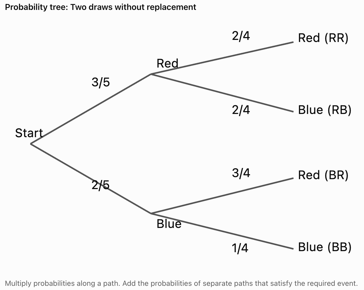
Calculating the Path Probabilities
Red, then red
P(RR) = 3/5 × 2/4
= 6/20 = 0.30
Red, then blue
P(RB) = 3/5 × 2/4
= 6/20 = 0.30
Blue, then red
P(BR) = 2/5 × 3/4
= 6/20 = 0.30
Blue, then blue
P(BB) = 2/5 × 1/4
= 2/20 = 0.10
The probabilities add to:
0.30 + 0.30 + 0.30 + 0.10 = 1
This confirms that all possible outcomes have been included.
Calculating Probabilities Involving Different Paths
Suppose we want the probability of selecting one red ball and one blue ball.
There are two possible sequences:
-
Red, then blue.
-
Blue, then red.
Therefore:
P(one red and one blue) = P(RB) + P(BR)
= 0.30 + 0.30
P(one red and one blue) = 0.60
There is a 60% probability of selecting one ball of each colour.
Important Principle
When solving multi-stage probability problems:
-
Multiply probabilities along a path.
-
Add probabilities for mutually exclusive paths that satisfy the event.
This principle is fundamental to probability tree diagrams.
Independent Events and the Multiplication Rule
Consider rolling two fair six-sided dice.
Let:
A = first die shows a 4
B = second die shows an even number
The events are independent.
P(A) = 1/6
P(B) = 3/6 = 1/2
Therefore:
P(A ∩ B) = 1/6 × 1/2
P(A ∩ B) = 1/12
There is an approximately 8.33% probability that the first die shows a 4 and the second die shows an even number.
Independent Events and the Addition Rule
Sometimes a problem asks for the probability that at least one of two events occurs.
The general addition rule is:
P(A ∪ B) = P(A) + P(B) − P(A ∩ B)
The symbol ∪ means "or."
The intersection is subtracted to avoid counting outcomes that satisfy both events twice.
Worked Example: At Least One Six
Two fair dice are rolled.
Find the probability that at least one die shows a 6.
Let:
A = first die shows a 6
B = second die shows a 6
P(A) = 1/6
P(B) = 1/6
P(A ∩ B) = 1/36
Therefore:
P(A ∪ B) = 1/6 + 1/6 − 1/36
= 6/36 + 6/36 − 1/36
P(A ∪ B) = 11/36 ≈ 0.3056
There is approximately a 30.56% probability that at least one die shows a 6.
Using Complementary Probability
Some probability problems are easier to solve using the complement.
The complement of an event A is the event that A does not occur.
P(not A) = 1 − P(A)
Worked Example: At Least One Head
A fair coin is tossed four times.
Find the probability of obtaining at least one head.
Instead of calculating the probabilities of one, two, three, or four heads separately, consider the opposite event.
The opposite of obtaining at least one head is obtaining no heads.
P(no heads) = (1/2)⁴
= 1/16
Therefore:
P(at least one head) = 1 − 1/16
P(at least one head) = 15/16 = 0.9375
There is a 93.75% probability of obtaining at least one head.
Independence Versus Mutual Exclusivity
Two events are mutually exclusive if they cannot occur at the same time.
For example, when rolling one die:
A = rolling a 2
B = rolling a 5
These events are mutually exclusive because one roll cannot produce both outcomes.
Therefore:
P(A ∩ B) = 0
However, these events are not independent.
If a 2 has occurred, the probability that the same roll is a 5 becomes zero.
Important Distinction
Independent events: One event does not change the probability of the other.
Mutually exclusive events: The two events cannot occur together.
For events with positive probabilities, mutual exclusivity and independence cannot both hold.
Comparison
|
Feature |
Independent events |
Mutually exclusive events |
|---|---|---|
|
Can both occur? |
Yes, if both have positive probability |
No |
|
Does one affect the other? |
No |
Yes, if both have positive probability |
|
Intersection probability |
P(A)P(B) |
0 |
|
Example |
Heads on two separate tosses |
Rolling a 2 and a 5 on one die |
Testing Whether Events Are Independent
Sometimes we are given probabilities and must determine whether two events are independent.
The test is:
P(A ∩ B) = P(A)P(B)
If this equality holds, the events are independent.
If it does not hold, the events are dependent.
Worked Example: Checking Independence
Suppose:
P(A) = 0.4
P(B) = 0.5
P(A ∩ B) = 0.2
Calculate:
P(A)P(B) = 0.4 × 0.5
= 0.2
Since:
P(A ∩ B) = P(A)P(B)
the events are independent.
A Dependent Example
Suppose instead:
P(A ∩ B) = 0.3
Then:
0.3 ≠ 0.4 × 0.5
Therefore, the events are dependent.
Using Two-Way Tables
Two-way tables are another useful method for analysing probability relationships.
Suppose 200 students are surveyed about participation in sports and music.
|
Plays music |
Does not play music |
Total |
|
|---|---|---|---|
|
Plays sports |
50 |
70 |
120 |
|
Does not play sports |
30 |
50 |
80 |
|
Total |
80 |
120 |
200 |
Let:
S = student plays sports
M = student plays music
Calculate the Individual Probabilities
P(S) = 120/200 = 0.60
P(M) = 80/200 = 0.40
Calculate the Joint Probability
P(S ∩ M) = 50/200
= 0.25
Test Independence
If the events were independent:
P(S)P(M) = 0.60 × 0.40
= 0.24
But:
P(S ∩ M) = 0.25
Since:
0.25 ≠ 0.24
the events are not exactly independent in this table.
Conditional Probability
P(M | S) = 50/120
≈ 0.4167
P(M) = 0.40
Knowing that a student plays sports changes the observed probability of playing music.
The table therefore shows dependence between these events.
This describes the observed data; a small difference alone does not establish a meaningful relationship in the wider population.
Probability with Three or More Events
The multiplication rule can be extended to several events.
For three events:
P(A ∩ B ∩ C) = P(A) × P(B | A) × P(C | A ∩ B)
This is called the chain rule of probability.
It accounts for how earlier events may affect later events.
If All Three Events Are Independent
Then:
P(A ∩ B ∩ C) = P(A) × P(B) × P(C)
Worked Example: Three Cards Without Replacement
Three cards are drawn from a standard deck without replacement.
Find the probability that all three are aces.
There are four aces in the deck.
First ace:
P(A₁) = 4/52
Second ace, given the first was an ace:
P(A₂ | A₁) = 3/51
Third ace, given the first two were aces:
P(A₃ | A₁ ∩ A₂) = 2/50
Multiply:
P(three aces) = 4/52 × 3/51 × 2/50
= 24/132600
P(three aces) = 1/5525 ≈ 0.000181
The probability is approximately 0.0181%.
Practical Application: Manufacturing Quality Control
A factory produces electronic components.
Suppose each component has a 2% probability of being defective, independently of the others.
Five components are selected.
Find the probability that all five are non-defective.
Step 1: Determine the Probability of a Non-Defective Component
P(non-defective) = 1 − 0.02
= 0.98
Step 2: Multiply
P(all five non-defective) = 0.98⁵
P(all five non-defective) ≈ 0.9039
There is approximately a 90.39% probability that all five components are non-defective.
Probability of At Least One Defect
Use complementary probability:
P(at least one defective) = 1 − 0.98⁵
P(at least one defective) ≈ 0.0961
There is approximately a 9.61% probability that at least one component is defective.
Practical Application: Medical Testing
Suppose a diagnostic test has a 95% probability of detecting a particular condition in someone who has it.
If two tests are conditionally independent given that the person has the condition, the probability that both tests are positive is:
P(both positive | condition) = 0.95 × 0.95
= 0.9025
There is a 90.25% probability of receiving two positive results under these assumptions.
Important Limitation
Medical tests may share sources of error.
For example, both tests may be affected by the same biological factor.
In that situation, the tests may not be conditionally independent.
Multiplying probabilities without checking the assumptions can produce misleading results.
Practical Application: Weather Events
Suppose a weather model estimates:
P(rain on Saturday) = 0.4
P(rain on Sunday) = 0.5
If the events were independent:
P(rain on both days) = 0.4 × 0.5
= 0.20
However, weather conditions often persist across multiple days.
Rain on Saturday may affect the probability of rain on Sunday.
If:
P(rain Sunday | rain Saturday) = 0.7
then:
P(rain both days) = 0.4 × 0.7
= 0.28
The dependent model produces a different result.
This illustrates why independence assumptions must be evaluated carefully.

Analysing Probability Models
A probability model represents uncertain events using mathematical assumptions.
When analysing a model, consider whether the events are independent or dependent.
Questions to Ask
-
Does the first event change the available outcomes?
-
Is an object replaced after being selected?
-
Do earlier results influence later results?
-
Are the events affected by common conditions?
-
Is the probability of each event constant?
-
Are the assumptions supported by the situation?
Example: Sampling Without Replacement
When sampling without replacement, probabilities generally change after each selection.
However, if the population is extremely large compared with the sample, the change may be very small.
In some applications, independence can be used as an approximation.
The accuracy of that approximation depends on the population size and sampling method.
Justifying Probability Calculations
A complete probability solution should include more than a numerical answer.
Students should explain why the chosen probability rule is appropriate.
Example of a Strong Justification
Two cards are drawn without replacement.
The probability of drawing two kings is:
P(two kings) = 4/52 × 3/51
= 1/221
The multiplication rule for dependent events is used because the first card is not replaced. After drawing one king, only three kings remain among 51 cards.
Why This Matters
A correct explanation demonstrates understanding of:
-
The events being considered.
-
The probability model.
-
Whether events are independent.
-
The mathematical rule being applied.
-
The meaning of the final result.
Justification is particularly important when solving complex probability problems.
Common Mistakes
Assuming events are independent because they happen separately
Separate events can still be dependent if they share underlying causes or influence one another.
Multiplying unconditional probabilities for dependent events
Use conditional probabilities when earlier events affect later ones.
Forgetting to adjust probabilities after drawing without replacement
Both the number of favourable outcomes and the total number of remaining outcomes may change.
Confusing independent and mutually exclusive events
Independent events do not influence one another, while mutually exclusive events cannot occur together.
Using addition instead of multiplication for joint events
When calculating the probability that events occur together, use the appropriate multiplication rule.
Forgetting to add separate valid paths
When an event can occur through multiple mutually exclusive sequences, calculate and add their probabilities.
Ignoring complementary probability
Problems involving at least one success are often easier to solve using the complement.
Assuming replacement always guarantees independence
Replacement can preserve probabilities in a well-shuffled random sampling experiment, but independence also depends on how the experiment is conducted.
Ignoring model assumptions
Real-world events may be influenced by shared conditions or changing probabilities.
Providing a numerical answer without justification
Probability calculations should include an explanation of why the method is appropriate.
Key Terms
-
Independent Events: Events where the occurrence of one does not change the probability of the other.
-
Dependent Events: Events where the occurrence of one changes the probability of the other.
-
Joint Probability: The probability that two or more events occur together.
-
Conditional Probability: The probability of an event occurring given that another event has occurred.
-
Intersection: The event that two or more specified events all occur.
-
Union: The event that at least one of two or more specified events occurs.
-
Multiplication Rule: A rule for calculating joint probabilities.
-
Addition Rule: A rule for calculating the probability of the union of events.
-
Mutually Exclusive Events: Events that cannot occur simultaneously.
-
Complementary Event: The event that a specified event does not occur.
-
Sample Space: The set of all possible outcomes of an experiment.
-
Probability Tree: A branching diagram showing possible sequences of events and their probabilities.
-
Two-Way Table: A table organizing frequencies or probabilities according to two categorical variables.
-
With Replacement: A sampling method in which an object is returned before the next selection.
-
Without Replacement: A sampling method in which selected objects are not returned before later selections.
-
Chain Rule of Probability: A multiplication rule expressing the probability of several events using conditional probabilities.
-
Conditional Independence: A relationship in which events are independent after conditioning on specified information.
-
Probability Model: A mathematical representation of uncertain outcomes.
-
Random Sampling: A method of selecting outcomes or individuals using a random process.
-
Independence Assumption: An assumption that one event does not influence the probability of another.
-
Complementary Probability: The probability of an event not occurring.
-
Bayesian Reasoning: Updating probabilities when new information becomes available.
-
Probability Justification: An explanation showing why a particular probability rule or calculation is appropriate.
Key Takeaways
-
Independent events do not change one another's probabilities.
-
Dependent events occur when the outcome of one event changes the probability of another.
-
The joint probability of independent events is P(A ∩ B) = P(A)P(B).
-
The general multiplication rule is P(A ∩ B) = P(A)P(B | A).
-
Conditional probability describes the probability of an event given that another event has occurred.
-
Drawing objects without replacement usually creates dependent events.
-
Drawing with replacement can produce independent events when the random sampling process remains unchanged.
-
Probability trees help organize multi-stage experiments.
-
Multiply probabilities along a probability-tree path.
-
Add probabilities for mutually exclusive paths that satisfy the event of interest.
-
The general addition rule is P(A ∪ B) = P(A) + P(B) − P(A ∩ B).
-
Complementary probability is useful for calculating the probability of at least one event occurring.
-
Independent events and mutually exclusive events are different concepts.
-
For events with positive probabilities, mutually exclusive events cannot be independent.
-
Two-way tables can be used to calculate conditional and joint probabilities.
-
The chain rule extends probability calculations to three or more events.
-
Real-world probability models must be evaluated for independence assumptions.
-
A complete probability solution should justify the chosen method and interpret the result.
Check Your Understanding
Recall and Understanding
-
Define independent events and provide an example.
-
Define dependent events and explain how they differ from independent events.
-
State the multiplication rule for independent events.
-
Explain the difference between independent and mutually exclusive events.
-
Describe how a probability tree can be used to calculate joint probabilities.
Application
-
Two fair coins are tossed. Calculate the probability that both show tails.
-
Two fair dice are rolled. Calculate the probability that the first die shows a 3 and the second shows an even number.
-
A bag contains four red balls and three blue balls. Two balls are drawn without replacement. Calculate the probability that both are red.
-
A standard deck contains 52 cards. Two cards are drawn without replacement. Calculate the probability that both are kings.
-
A machine produces components with a 3% probability of being defective, independently of one another. Calculate the probability that all four selected components are non-defective.
Analysis and Challenge
-
A bag contains five red balls, three blue balls, and two green balls. Two balls are drawn without replacement. Calculate the probability that one is red and the other is blue, in either order.
-
Suppose P(A) = 0.6, P(B) = 0.4, and P(A ∩ B) = 0.24. Determine whether A and B are independent and justify your answer.
-
A school survey finds that 80 students play sports, 60 play music, and 30 do both, out of 150 students. Determine whether playing sports and playing music are independent events in the survey data.
-
Three cards are drawn from a standard deck without replacement. Calculate the probability that all three are hearts.
-
A factory uses two machines. Machine A produces 60% of the products and Machine B produces 40%. Machine A has a 2% defect rate, while Machine B has a 5% defect rate. Calculate the probability that a randomly selected product is defective, and explain why the relevant events must be treated carefully when constructing the probability model.
Final Summary
Independent and dependent events are fundamental concepts in probability.
Independent events do not influence one another's probabilities, while dependent events involve changes in probability based on earlier outcomes or additional information.
By applying multiplication rules, conditional probabilities, probability trees, and complementary probability, students can calculate joint probabilities and solve problems involving multiple events.
The distinction between independence and dependence is especially important in sampling, manufacturing, medical testing, weather forecasting, and scientific investigations.
Understanding how events interact allows students to select appropriate probability models, justify calculations, and interpret uncertain situations accurately.
3. Markov Processes
Learning outcomes
- I can describe simple Markov processes.
- I can interpret transition diagrams.
- I can calculate transition probabilities.
- I can model simple stochastic systems.
- I can apply Markov models to practical situations.
Markov Processes
Introduction to Markov Processes
Many real-world situations involve systems that change over time. The changes are not always predictable, but the probabilities of different outcomes can often be estimated.
Consider the following situations:
-
Tomorrow's weather may depend on today's weather.
-
A customer may continue using a product or switch to another brand.
-
A machine may remain operational or develop a fault.
-
An animal may move between different habitats.
-
A student may progress between different levels of understanding.
These situations can be studied using Markov processes.
A Markov process is a mathematical model describing a system that moves between different states according to probabilities.
The defining feature is that the probability of the next state depends on the current state, rather than the complete history of previous states.
This is called the Markov property.
Markov models are widely used in mathematics, science, economics, computing, engineering, and environmental research.


Understanding Stochastic Processes
A stochastic process is a mathematical model describing a system that changes over time in a way that involves randomness.
The word stochastic means that chance or probability influences the outcomes.
For example, consider the weather over several days.
The weather may be:
-
Sunny
-
Cloudy
-
Rainy
The weather tomorrow is uncertain, even when today's weather is known.
However, past observations may help us estimate the probability of each possible outcome.
A stochastic process describes how these uncertain changes occur.
Deterministic Versus Stochastic Systems
A deterministic system produces an outcome that is completely determined by its initial conditions and governing rules.
A stochastic system includes uncertainty, so the same current conditions can lead to different outcomes.
|
Deterministic system |
Stochastic system |
|---|---|
|
Next state is fixed by the model |
Next state is selected according to probabilities |
|
Same starting conditions give the same result |
Same starting state can lead to different results |
|
Example: a fixed numerical sequence |
Example: a probabilistic weather model |
Markov processes are a particular type of stochastic process.
The Markov Property
The central idea of a Markov process is that the future depends on the present state, not on the full history of previous states.
This is sometimes called the memoryless property.
For a sequence of states X₀, X₁, X₂, ...:
P(Xₙ₊₁ = j | Xₙ = i, earlier states) = P(Xₙ₊₁ = j | Xₙ = i)
This means that once the current state is known, earlier states provide no additional information about the probability of the next state.
Example: Weather
Suppose a simplified weather model contains two states:
-
Sunny
-
Rainy
If today is sunny, the probability of tomorrow being rainy is 0.3.
In a Markov model, this probability remains 0.3 regardless of whether yesterday was sunny or rainy.
The model uses today's weather to predict tomorrow's weather.
Important Limitation
Real weather depends on many variables, including atmospheric pressure, temperature, humidity, and wind.
A simple two-state Markov model is therefore an approximation.
Its usefulness depends on whether the chosen states contain enough information to make reasonable predictions.
States in a Markov Process
A state describes the condition of a system at a particular time.
Examples include:
|
System |
Possible states |
|---|---|
|
Weather |
Sunny, cloudy, rainy |
|
Machine |
Working, broken |
|
Customer behaviour |
Brand A, Brand B |
|
Student progress |
Beginning, developing, proficient |
|
Animal movement |
Forest, grassland, wetland |
|
Traffic |
Light, moderate, heavy |
A Markov model requires a clearly defined set of states.
Important Requirements
The states should be:
-
Clearly defined.
-
Mutually exclusive at a given observation time.
-
Sufficient to describe the modelled system.
-
Appropriate for the question being investigated.
For example, if weather states are defined as sunny and rainy, the model must specify how cloudy conditions are classified.
Otherwise, the states may not cover all possible outcomes.
Transition Probabilities
A transition probability describes the probability that a system moves from one state to another during a specified time step.
For example, suppose a weather model has the following probabilities:
-
If today is sunny, tomorrow is sunny with probability 0.7.
-
If today is sunny, tomorrow is rainy with probability 0.3.
-
If today is rainy, tomorrow is sunny with probability 0.4.
-
If today is rainy, tomorrow is rainy with probability 0.6.
These probabilities describe transitions between the two weather states.
Transition Probability Table
|
Current state |
Next day sunny |
Next day rainy |
|---|---|---|
|
Sunny |
0.7 |
0.3 |
|
Rainy |
0.4 |
0.6 |
Each row represents the probabilities of the possible next states, given the current state.
Important Rule
The transition probabilities leaving each state must add to 1.
For sunny weather:
0.7 + 0.3 = 1
For rainy weather:
0.4 + 0.6 = 1
This ensures that the next state must be one of the possible states in the model.
Transition Diagrams
A transition diagram is a visual representation of a Markov process.
Each state is represented by a circle or node.
Arrows show possible transitions between states.
The numbers on the arrows represent transition probabilities.
Example: Sunny and Rainy Weather
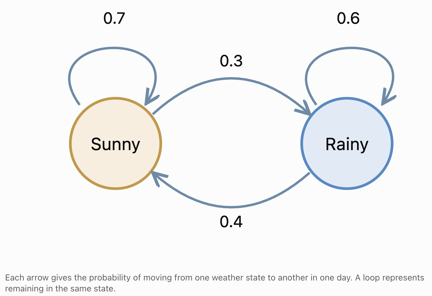
Interpreting the Diagram
The arrow from Sunny to Rainy has probability 0.3.
This means:
P(Rainy tomorrow | Sunny today) = 0.3
The loop from Sunny back to Sunny has probability 0.7.
This means:
P(Sunny tomorrow | Sunny today) = 0.7
Similarly:
P(Sunny tomorrow | Rainy today) = 0.4
P(Rainy tomorrow | Rainy today) = 0.6
Transition Matrices
A transition matrix organizes transition probabilities into a rectangular array.
For the weather model, we can write:
P = [[0.7, 0.3], [0.4, 0.6]]
The rows represent the current state.
The columns represent the next state.
We will use the state order:
Sunny, Rainy
|
Sunny next |
Rainy next |
|
|---|---|---|
|
Sunny now |
0.7 |
0.3 |
|
Rainy now |
0.4 |
0.6 |
Properties of a Transition Matrix
For a finite-state Markov chain using this row convention:
-
Every entry is between 0 and 1.
-
Every row adds to 1.
-
Each row describes the probabilities of leaving one state.
-
Each column identifies the destination state.
A matrix satisfying these conditions is called a row-stochastic matrix.
Why Matrices Are Useful
Transition matrices allow us to calculate probabilities over several time steps.
They are particularly useful when a model contains many states.
Calculating One-Step Transition Probabilities
Suppose today is sunny.
Using the weather transition matrix:
P = [[0.7, 0.3], [0.4, 0.6]]
The probability that tomorrow is sunny is:
P(Sunny tomorrow | Sunny today) = 0.7
The probability that tomorrow is rainy is:
P(Rainy tomorrow | Sunny today) = 0.3
If today is rainy:
P(Sunny tomorrow | Rainy today) = 0.4
P(Rainy tomorrow | Rainy today) = 0.6
These are called one-step transition probabilities because they describe changes over one time interval.
Calculating Two-Step Transition Probabilities
Markov models can also be used to predict states several steps into the future.
Suppose today is sunny.
What is the probability that the weather will be sunny two days from now?
There are two possible paths ending in sunny weather:
-
Sunny → Sunny → Sunny
-
Sunny → Rainy → Sunny
Path One: Sunny, Sunny, Sunny
Probability:
0.7 × 0.7 = 0.49
Path Two: Sunny, Rainy, Sunny
Probability:
0.3 × 0.4 = 0.12
Add the Probabilities
P(Sunny in two days | Sunny today) = 0.49 + 0.12
= 0.61
There is a 61% probability that the weather will be sunny two days from now.
Why Do We Add the Paths?
The two paths are mutually exclusive.
The system cannot be both sunny and rainy on the intermediate day.
Therefore, the probabilities of the separate paths can be added.
Worked Example: Rain Two Days from Now
Suppose today is sunny.
Find the probability that it will be rainy two days from now.
Possible paths:
-
Sunny → Sunny → Rainy
-
Sunny → Rainy → Rainy
First path:
0.7 × 0.3 = 0.21
Second path:
0.3 × 0.6 = 0.18
Add:
P(Rainy in two days | Sunny today) = 0.21 + 0.18
= 0.39
The two-day probabilities are:
-
Sunny: 0.61
-
Rainy: 0.39
Check:
0.61 + 0.39 = 1
The results form a valid probability distribution.
Matrix Multiplication and Markov Processes
Transition matrices can be multiplied to calculate multi-step probabilities.
For the weather model:
P = [[0.7, 0.3], [0.4, 0.6]]
The two-step transition matrix is:
P² = P × P
Calculate each entry by multiplying corresponding row and column values and adding the results.
Sunny to Sunny
0.7 × 0.7 + 0.3 × 0.4
= 0.49 + 0.12
= 0.61
Sunny to Rainy
0.7 × 0.3 + 0.3 × 0.6
= 0.21 + 0.18
= 0.39
Rainy to Sunny
0.4 × 0.7 + 0.6 × 0.4
= 0.28 + 0.24
= 0.52
Rainy to Rainy
0.4 × 0.3 + 0.6 × 0.6
= 0.12 + 0.36
= 0.48
Therefore:
P² = [[0.61, 0.39], [0.52, 0.48]]
|
Starting state |
Sunny after two days |
Rainy after two days |
|---|---|---|
|
Sunny |
0.61 |
0.39 |
|
Rainy |
0.52 |
0.48 |
Notice that the rows still add to 1.
Calculating Three-Step and Longer-Term Probabilities
The same principle extends to additional time steps.
P³ = P² × P
More generally:
Pⁿ = n-step transition matrix
where n is a positive integer.
For the weather model:
P³ = [[0.583, 0.417], [0.556, 0.444]]
Therefore, if today is sunny:
P(Sunny in three days) = 0.583
P(Rainy in three days) = 0.417
The transition matrix can be raised to higher powers to calculate probabilities over many days.
This makes Markov processes useful for forecasting.
State Probability Distributions
Sometimes the current state is uncertain.
Instead of knowing that today is sunny, we might know the probabilities of the current states.
Suppose:
-
Probability of sunny today = 0.6
-
Probability of rainy today = 0.4
We can represent this as a state probability vector:
v₀ = [0.6, 0.4]
The entries represent the probabilities of the states in the chosen order.
Calculating Tomorrow's State Distribution
Using the row-vector convention:
v₁ = v₀P
Substitute:
v₁ = [0.6, 0.4] × [[0.7, 0.3], [0.4, 0.6]]
Sunny probability:
0.6 × 0.7 + 0.4 × 0.4
= 0.42 + 0.16
= 0.58
Rainy probability:
0.6 × 0.3 + 0.4 × 0.6
= 0.18 + 0.24
= 0.42
Therefore:
v₁ = [0.58, 0.42]
Tomorrow's predicted state probabilities are:
-
Sunny: 58%
-
Rainy: 42%
General Formula
For n time steps:
vₙ = v₀Pⁿ
This formula allows us to predict the probability distribution of states at future times.
Modelling a Simple Stochastic System
Consider a machine that can be in one of two states:
-
Working
-
Broken
Suppose:
-
A working machine remains working the next day with probability 0.9.
-
A working machine becomes broken with probability 0.1.
-
A broken machine is repaired and working the next day with probability 0.6.
-
A broken machine remains broken with probability 0.4.
Transition Matrix
Using the state order Working, Broken:
P = [[0.9, 0.1], [0.6, 0.4]]
One-Step Interpretation
If the machine is working today:
P(Working tomorrow) = 0.9
P(Broken tomorrow) = 0.1
If the machine is broken today:
P(Working tomorrow) = 0.6
P(Broken tomorrow) = 0.4
Two-Step Probability of Remaining Operational
Suppose the machine is working today.
What is the probability that it is working two days from now?
There are two possible paths:
Working → Working → Working
Working → Broken → Working
Calculate:
P(Working after two days) = 0.9 × 0.9 + 0.1 × 0.6
= 0.81 + 0.06
= 0.87
There is an 87% probability that the machine will be working two days from now.

Absorbing States
An absorbing state is a state that cannot be left once the system enters it.
The probability of remaining in an absorbing state is 1.
Example: Equipment Failure Without Repair
Suppose a machine can be:
-
Working
-
Permanently failed
Once the machine permanently fails, it cannot return to the working state.
The transition matrix might be:
P = [[0.95, 0.05], [0, 1]]
|
Current state |
Working next |
Failed next |
|---|---|---|
|
Working |
0.95 |
0.05 |
|
Failed |
0 |
1 |
The failed state is absorbing because:
P(Failed next | Failed now) = 1
Applications of Absorbing States
Absorbing states are useful for modelling:
-
Permanent equipment failure.
-
Completion of a task.
-
Graduation from a programme.
-
Reaching a final stage in a game.
-
Extinction of a population in a simplified ecological model.
Steady-State Probabilities
Some Markov chains approach a stable probability distribution over time.
This is called a steady-state distribution or stationary distribution.
A stationary distribution remains unchanged after one transition.
If π is a stationary distribution, then:
πP = π
The entries of π must also add to 1.
Worked Example: Long-Term Weather Probabilities
Recall the weather transition matrix:
P = [[0.7, 0.3], [0.4, 0.6]]
Let:
s = long-term probability of sunny weather
r = long-term probability of rainy weather
We know:
s + r = 1
At steady state:
s = 0.7s + 0.4r
Rearrange:
0.3s = 0.4r
Therefore:
3s = 4r
So:
s = (4/3)r
Substitute into:
s + r = 1
(4/3)r + r = 1
(7/3)r = 1
r = 3/7
Therefore:
s = 4/7
Final Answer
Sunny ≈ 57.14%
Rainy ≈ 42.86%
In this model, the long-term state distribution approaches approximately 57.14% sunny and 42.86% rainy.
Important Distinction
A steady-state distribution does not mean the weather stops changing.
The system continues moving between sunny and rainy states.
The long-term probabilities become stable even though individual outcomes remain uncertain.
Not every Markov chain converges to a unique stationary distribution from every starting state.
Practical Application: Customer Brand Loyalty
Businesses can use Markov models to study customer behaviour.
Suppose customers choose between two brands:
-
Brand A
-
Brand B
Each month:
-
80% of Brand A customers remain with Brand A.
-
20% switch to Brand B.
-
30% of Brand B customers switch to Brand A.
-
70% remain with Brand B.
Transition Matrix
P = [[0.8, 0.2], [0.3, 0.7]]
Suppose the initial market shares are:
Brand A = 60%
Brand B = 40%
The initial state vector is:
v₀ = [0.6, 0.4]
Calculate Next Month's Market Shares
v₁ = v₀P
Brand A:
0.6 × 0.8 + 0.4 × 0.3
= 0.48 + 0.12
= 0.60
Brand B:
0.6 × 0.2 + 0.4 × 0.7
= 0.12 + 0.28
= 0.40
Therefore:
v₁ = [0.6, 0.4]
The market shares remain unchanged.
This initial distribution is already a stationary distribution for the model.
Interpretation
Even though some customers switch brands each month, the overall market shares can remain constant.
This demonstrates how a system can experience individual changes while maintaining stable overall proportions.

Practical Application: Animal Movement
Ecologists can use Markov processes to model animal movement between habitats.
Suppose a population of animals moves between:
-
Forest
-
Grassland
Each day:
-
85% of animals in the forest remain there.
-
15% move to grassland.
-
25% of animals in grassland move to forest.
-
75% remain in grassland.
The transition matrix is:
P = [[0.85, 0.15], [0.25, 0.75]]
Suppose initially:
-
70% of animals are in the forest.
-
30% are in grassland.
Then:
v₀ = [0.7, 0.3]
Predict the Next Day
Forest:
0.7 × 0.85 + 0.3 × 0.25
= 0.595 + 0.075
= 0.67
Grassland:
0.7 × 0.15 + 0.3 × 0.75
= 0.105 + 0.225
= 0.33
Therefore:
v₁ = [0.67, 0.33]
The model predicts:
-
67% in forest.
-
33% in grassland.
Real-World Limitations
Actual animal movement may depend on:
-
Food availability.
-
Weather.
-
Predators.
-
Seasonal changes.
-
Habitat destruction.
-
Reproductive behaviour.
A simple Markov model may need additional states or changing transition probabilities to represent these factors accurately.

Practical Application: Student Learning Progress
Markov models can also describe movement between learning stages.
Suppose students are classified into three states:
-
Beginning
-
Developing
-
Proficient
A simplified transition matrix might be:
|
Current level |
Beginning next |
Developing next |
Proficient next |
|---|---|---|---|
|
Beginning |
0.5 |
0.4 |
0.1 |
|
Developing |
0.1 |
0.6 |
0.3 |
|
Proficient |
0.02 |
0.08 |
0.90 |
Each row adds to 1.
For example, a student currently at the Developing level has:
-
10% probability of moving to Beginning.
-
60% probability of remaining Developing.
-
30% probability of moving to Proficient.
Interpretation
A school could use such a model to estimate future distributions of achievement levels.
However, learning is influenced by teaching quality, motivation, prior knowledge, attendance, and other factors.
A simple Markov model should not be interpreted as a fixed prediction of an individual student's future achievement.
Time-Homogeneous and Time-Varying Markov Chains
Many introductory Markov models assume that transition probabilities remain constant over time.
These are called time-homogeneous Markov chains.
For example:
P(Sunny tomorrow | Sunny today) = 0.7
remains the same throughout the model.
However, some real systems change over time.
Time-Varying Example
A machine may become more likely to fail as it ages.
Its transition probabilities may therefore change each month.
Similarly, animal movement probabilities may change with the seasons.
Such systems can be modelled using different transition matrices at different time steps.
Important Distinction
The Markov property does not require transition probabilities to remain constant over time.
It requires that the next-state probabilities depend on the current state rather than the complete past history.
Evaluating Markov Models
Markov models simplify complex systems.
Their usefulness depends on whether the assumptions reasonably describe the situation.
Questions to Consider
Are the states clearly defined?
Every possible situation should correspond to an appropriate state.
Does the current state contain enough information?
If earlier history influences the future beyond what is represented by the current state, the simple Markov assumption may be unsuitable.
Are the transition probabilities realistic?
Probabilities should be estimated using suitable observations or justified assumptions.
Do the probabilities add to 1?
Every row of the transition matrix must add to 1.
Are transition probabilities constant?
If not, a time-varying model may be needed.
Does the model accurately represent the system?
Predictions should be compared with real observations when possible.
A Strategy for Solving Markov Problems
When solving a Markov process problem, use the following steps.
Identify the states.
Determine the possible conditions of the system.
Choose a consistent state order.
For example:
Sunny, Rainy
Identify the transition probabilities.
Determine the probability of moving from each current state to every possible next state.
Construct the transition matrix.
Place the current states in rows and next states in columns.
Check the matrix.
Ensure all entries are between 0 and 1 and each row adds to 1.
Determine the initial state.
The initial state may be known exactly or represented by a probability distribution.
Calculate the required probabilities.
Use probability paths, matrix multiplication, or state vectors.
Interpret the results.
Explain what the calculated probabilities mean in the context of the problem.
Evaluate the model.
Consider whether the assumptions are realistic.
Common Mistakes
Confusing a Markov process with a deterministic process
A Markov process describes probabilistic transitions rather than guaranteed outcomes.
Assuming the future is independent of the present
The Markov property means that the future depends on the current state, not that all states are independent.
Confusing the Markov property with complete randomness
Markov processes can contain strong relationships between consecutive states.
Reading a transition matrix incorrectly
Always identify whether rows or columns represent the current state.
Forgetting that transition probabilities must add to 1
Every row must represent a complete probability distribution of possible next states.
Multiplying transition probabilities incorrectly
For multi-step transitions, consider every possible intermediate state.
Forgetting to add alternative paths
Different paths may lead to the same final state.
Confusing one-step and two-step probabilities
P gives one-step transitions, while P² gives two-step transitions.
Assuming a steady state means no changes occur
A stationary distribution can remain constant even while individual states continue changing.
Assuming every Markov chain reaches the same steady state
Some chains do not converge to a unique stationary distribution.
Ignoring real-world limitations
Actual systems may require more states, additional variables, or changing transition probabilities.
Key Terms
-
Markov Process: A stochastic process in which the next-state probabilities depend on the current state rather than the complete history.
-
Markov Chain: A Markov process with a discrete set of states and discrete time steps.
-
Stochastic Process: A mathematical model describing a system that changes over time with an element of randomness.
-
Deterministic Process: A process whose future states are fully determined by its current conditions and rules.
-
State: A possible condition of a system at a particular time.
-
State Space: The set of all possible states in a model.
-
Markov Property: The property that the current state contains all information from the past needed to predict the next state.
-
Transition: A movement from one state to another.
-
Transition Probability: The probability of moving from one state to another during a specified time step.
-
Transition Diagram: A diagram showing states as nodes and transitions as arrows.
-
Transition Matrix: A matrix containing the probabilities of moving between states.
-
Stochastic Matrix: A matrix containing non-negative probabilities whose rows or columns sum to 1, depending on the convention.
-
Row-Stochastic Matrix: A transition matrix in which every row sums to 1.
-
One-Step Probability: The probability of moving between states in one time interval.
-
Multi-Step Probability: The probability of moving between states over several time intervals.
-
State Vector: A vector describing the probabilities of the possible states at a particular time.
-
Initial Distribution: The probability distribution of states at the beginning of a process.
-
Matrix Multiplication: A mathematical operation used to combine transition probabilities.
-
Absorbing State: A state that cannot be left once entered.
-
Stationary Distribution: A probability distribution that remains unchanged after applying the transition matrix.
-
Steady State: A stable probability distribution that may describe the long-term behaviour of a Markov chain.
-
Time-Homogeneous Markov Chain: A Markov chain whose transition probabilities remain constant over time.
-
Time-Varying Markov Chain: A Markov chain whose transition probabilities can change over time.
-
Probability Model: A mathematical representation of uncertain outcomes.
-
Stochastic Modelling: The use of mathematical models to describe systems involving randomness.
Key Takeaways
-
Markov processes describe systems that move between states according to probabilities.
-
The Markov property states that the next state depends on the current state rather than the complete history.
-
Markov chains are commonly used to model systems with discrete states and discrete time steps.
-
Transition probabilities describe the likelihood of moving from one state to another.
-
Transition diagrams use nodes and arrows to represent states and transitions.
-
Transition matrices organize transition probabilities into rows and columns.
-
In a row-stochastic transition matrix, every row must add to 1.
-
One-step transition probabilities describe changes over one time interval.
-
Two-step probabilities can be calculated by considering all possible intermediate states.
-
Matrix multiplication provides an efficient way to calculate multi-step probabilities.
-
P² represents two-step transition probabilities, while Pⁿ represents n-step probabilities.
-
State vectors describe the probability distribution of the system across its possible states.
-
The formula vₙ = v₀Pⁿ predicts state distributions after n time steps using the row-vector convention.
-
Absorbing states cannot be left once entered.
-
Some Markov chains approach stable long-term probability distributions.
-
A stationary distribution satisfies πP = π.
-
A steady-state distribution does not mean that individual state changes stop.
-
Markov models are useful in weather forecasting, manufacturing, ecology, customer behaviour, education, and engineering.
-
The accuracy of a Markov model depends on its assumptions, state definitions, and transition probabilities.
Check Your Understanding
Recall and Understanding
-
Define a Markov process and explain the Markov property.
-
Explain the difference between a deterministic process and a stochastic process.
-
Define a state and a transition probability.
-
Explain how a transition diagram represents a Markov chain.
-
State the requirements for a valid row-stochastic transition matrix.
Application
-
A weather model has two states, Sunny and Rainy. If P(Sunny → Sunny) = 0.8 and P(Rainy → Sunny) = 0.3, construct the transition matrix.
-
A machine has a 90% probability of remaining operational and a 10% probability of failing each day when working. A failed machine has a 60% probability of being repaired by the next day. Construct a transition matrix.
-
Using the weather matrix P = [[0.7, 0.3], [0.4, 0.6]], calculate the probability that it is sunny two days from now if today is rainy.
-
A Markov chain has transition matrix P = [[0.6, 0.4], [0.2, 0.8]]. Calculate P².
-
A system has initial state vector v₀ = [0.3, 0.7] and transition matrix P = [[0.8, 0.2], [0.5, 0.5]]. Calculate the state distribution after one step.
Analysis and Challenge
-
A customer loyalty model has transition matrix P = [[0.85, 0.15], [0.25, 0.75]]. If 60% of customers initially use Brand A, calculate the expected market shares after two months.
-
Explain why the Markov property does not mean that consecutive states are independent.
-
A machine has states Working and Permanently Failed, with transition matrix P = [[0.95, 0.05], [0, 1]]. Identify the absorbing state and calculate the probability that a machine working initially has permanently failed after two time steps.
-
Find the stationary distribution for the transition matrix P = [[0.8, 0.2], [0.3, 0.7]].
-
Design a simple three-state Markov model for student learning progress, animal movement, or weather conditions. Construct a valid transition matrix, explain your probabilities, and describe one limitation of your model.
Final Summary
Markov processes provide a mathematical framework for describing systems that change between states according to probabilities.
The defining feature of a Markov process is that the next-state probabilities depend on the current state rather than the complete history of previous states.
Transition diagrams and transition matrices allow these probabilities to be represented clearly.
By multiplying transition matrices and using state probability vectors, we can calculate the likelihood of future states and investigate long-term behaviour.
Markov models are valuable tools for analysing weather patterns, equipment reliability, customer behaviour, animal movement, and other systems involving uncertainty.
Understanding their assumptions and limitations is essential for constructing useful models and interpreting their predictions accurately.
4. Simulation and Monte Carlo Methods
Learning outcomes
- I can explain simulation techniques.
- I can perform Monte Carlo simulations.
- I can estimate probabilities experimentally.
- I can compare theoretical and simulated results.
- I can evaluate simulation accuracy.
Simulation and Monte Carlo Methods
Introduction to Simulation and Monte Carlo Methods
Many real-world situations involve uncertainty. Sometimes probabilities can be calculated exactly using mathematical formulas, but other problems are too complicated for a simple theoretical solution.
For example:
-
What is the probability of winning a particular board game?
-
How likely is a project to finish before its deadline?
-
What is the chance that a machine will fail during a given period?
-
How often will a particular combination of dice rolls occur?
-
How accurately can we estimate an area using randomly generated points?
One approach is to create a mathematical or computer-based model and repeat an experiment many times.
This process is called simulation.
A particularly important simulation technique is the Monte Carlo method, which uses random sampling and repeated trials to estimate probabilities or numerical quantities.
Simulation is widely used in science, engineering, finance, medicine, weather forecasting, computer science, and probability research.


What Is a Simulation?
A simulation is a model that imitates the behaviour of a real or hypothetical system.
Instead of observing the actual system repeatedly, we reproduce its important features using mathematical rules, physical objects, or computer programs.
A simulation might involve:
-
Tossing coins.
-
Rolling dice.
-
Drawing numbered cards.
-
Generating random numbers.
-
Using spreadsheet formulas.
-
Running a computer program.
Example: Simulating Coin Tosses
Suppose we want to estimate the probability of obtaining heads when tossing a fair coin.
We could toss a real coin 100 times and record the outcomes.
Alternatively, we could use a random number generator:
-
Generate 0 to represent tails.
-
Generate 1 to represent heads.
Repeating this process many times produces a simulated coin-toss experiment.
The proportion of heads can then be compared with the theoretical probability of 0.5.
Theoretical and Experimental Probability
Theoretical Probability
Theoretical probability is calculated using a mathematical model.
For equally likely outcomes:
P(E) = Number of favourable outcomes / Total number of possible outcomes
For example, the probability of rolling a 6 on a fair die is:
P(6) = 1/6
≈ 0.1667
Experimental Probability
Experimental probability is estimated from observations or repeated trials.
Experimental probability = Number of times event occurs / Total number of trials
For example, suppose a die is rolled 120 times and a 6 appears 23 times.
Experimental probability:
P(6) ≈ 23/120
P(6) ≈ 0.1917
This differs from the theoretical probability of approximately 0.1667.
The difference is expected because random experiments produce variation.
What Is a Monte Carlo Simulation?
A Monte Carlo simulation is a method that uses random sampling to investigate a mathematical or real-world problem.
The method generally involves:
-
Defining a problem.
-
Creating a mathematical model.
-
Generating random inputs.
-
Repeating the experiment many times.
-
Recording the outcomes.
-
Using the results to estimate probabilities or other quantities.
The name Monte Carlo refers to the famous casino district in Monaco, reflecting the importance of randomness in the method.
Monte Carlo methods are especially useful when exact calculations are difficult or when a system contains several uncertain variables.
The Monte Carlo Simulation Process
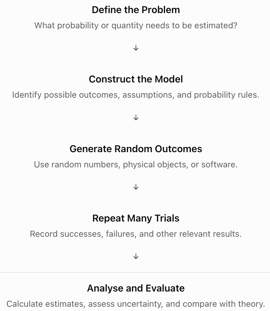
Performing a Simple Coin-Toss Simulation
Suppose we want to estimate the probability of obtaining heads on a fair coin.
Step 1: Define the Outcomes
The possible outcomes are:
-
Heads
-
Tails
The theoretical probabilities are:
P(Heads) = 0.5
P(Tails) = 0.5
Step 2: Simulate the Experiment
Generate random outcomes representing heads or tails.
Step 3: Record the Results
Suppose a simulation produces the following illustrative results:
|
Number of tosses |
Heads observed |
Experimental probability |
|---|---|---|
|
10 |
7 |
0.700 |
|
50 |
28 |
0.560 |
|
100 |
53 |
0.530 |
|
500 |
247 |
0.494 |
|
1,000 |
503 |
0.503 |
|
10,000 |
5,012 |
0.5012 |
These are example results, not guaranteed outcomes of a simulation.
Step 4: Compare With Theory
The theoretical probability is:
P(Heads) = 0.5
As the number of trials increases, the experimental probability often becomes closer to 0.5.
However, random fluctuations remain possible.
Interactive Coin-Toss Simulation
Try simulating a fair coin below. Each batch adds new trials, allowing you to observe how the estimated probability changes.
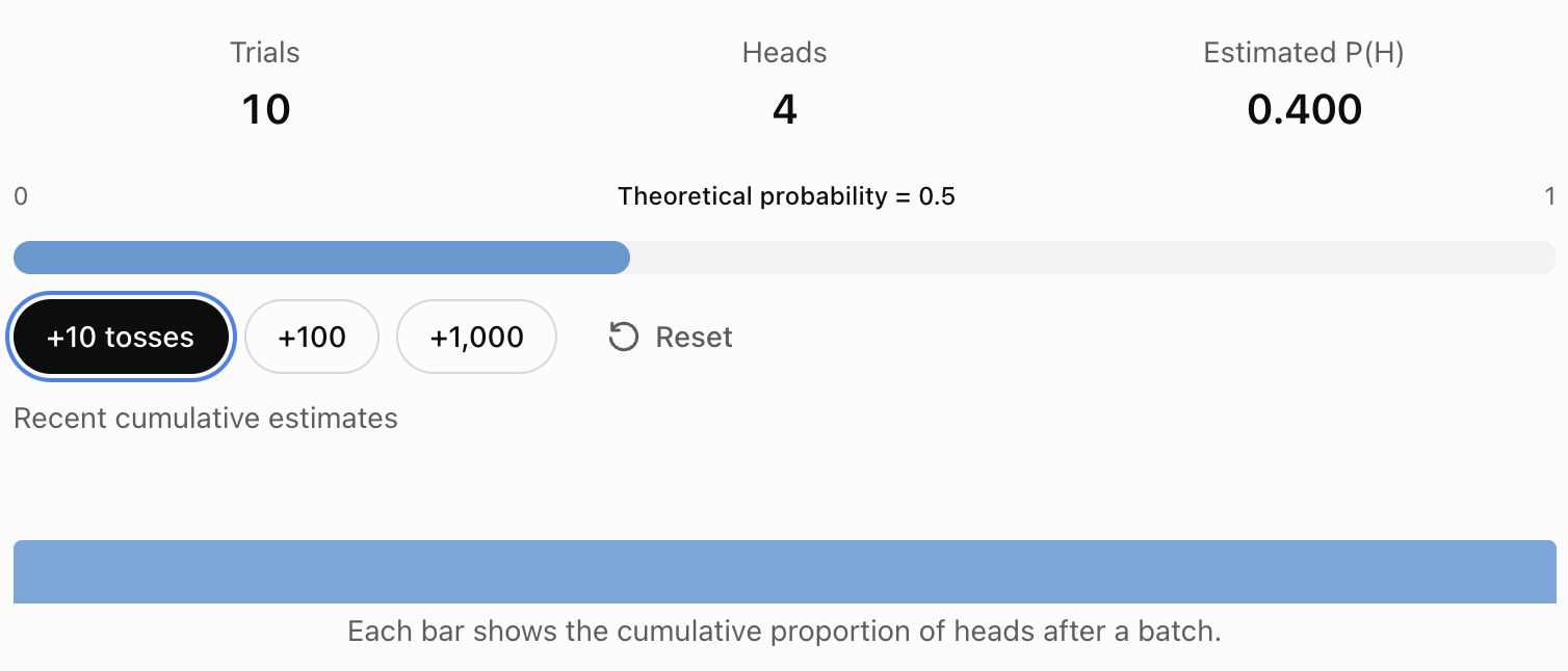
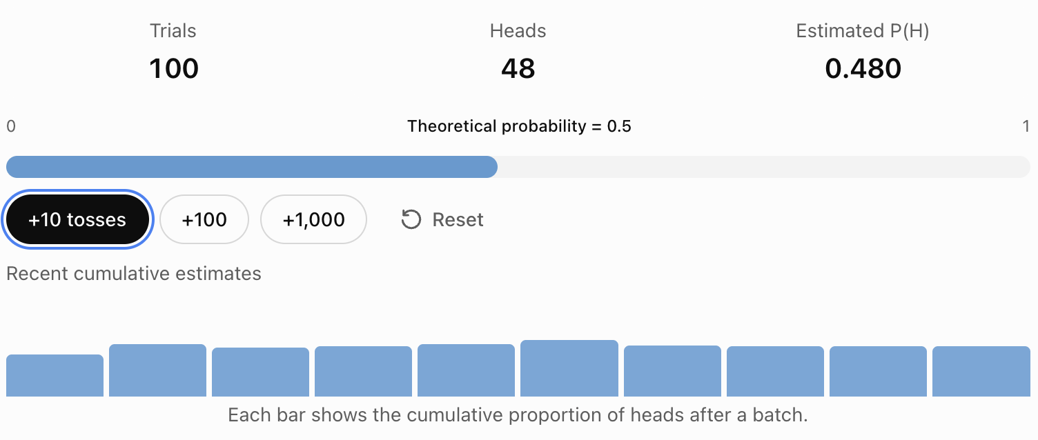
The estimate should generally become more stable as the number of tosses increases, although it will not necessarily move closer to 0.5 after every batch.
The Law of Large Numbers
The Law of Large Numbers states that, under appropriate conditions, the average result of many independent repetitions approaches the expected value as the number of trials increases.
For a fair coin:
Expected proportion of heads = 0.5
As more tosses are performed, the observed proportion tends to approach 0.5.
Important Distinction
The Law of Large Numbers does not mean that the number of heads and tails must become equal.
For example, after 10,000 tosses, it is possible to have:
-
5,080 heads.
-
4,920 tails.
The difference is 160 tosses.
However, the proportion of heads is:
5,080/10,000 = 0.508
This is relatively close to the theoretical probability of 0.5.
The absolute difference between the counts may increase even while the relative frequencies become more stable.
Simulating Dice Rolls
Suppose we want to estimate the probability of rolling a total of 7 with two fair dice.
Theoretical Probability
Each die has six possible outcomes.
The total number of equally likely ordered outcomes is:
6 × 6 = 36
The combinations producing a total of 7 are:
(1,6), (2,5), (3,4), (4,3), (5,2), (6,1)
There are six favourable outcomes.
Therefore:
P(sum = 7) = 6/36
P(sum = 7) = 1/6 ≈ 0.1667
Monte Carlo Method
A simulation would:
-
Generate a random integer from 1 to 6.
-
Generate a second independent random integer from 1 to 6.
-
Add the two values.
-
Record whether the sum equals 7.
-
Repeat thousands of times.
Suppose the simulation produces 1,681 successes in 10,000 trials.
Experimental probability:
P(sum = 7) ≈ 1681/10000
P(sum = 7) ≈ 0.1681
The simulated result is close to the theoretical probability of approximately 0.1667.

Simulating Events with Unequal Probabilities
Not all simulations involve equally likely outcomes.
Suppose a basketball player has a 70% probability of making a free throw.
We can simulate each attempt using a random number between 0 and 1.
Define:
-
Random number below 0.70 → successful shot.
-
Random number at least 0.70 → missed shot.
If the random number generator produces values uniformly between 0 and 1, this gives the required success probability.
Example
Suppose the generated random numbers are:
0.24, 0.83, 0.65, 0.11, 0.92
The corresponding outcomes are:
Success, Miss, Success, Success, Miss
Three successes occur in five attempts.
Experimental success rate:
3/5 = 0.60
Although the theoretical success probability is 0.70, a small sample can produce a different result.
Monte Carlo Simulation of a Binomial Experiment
Suppose a basketball player makes each independent free throw with probability 0.7.
The player attempts ten shots.
We want to estimate:
P(exactly 7 successful shots)
Theoretical Calculation
The number of successes follows a binomial distribution:
X ~ B(10, 0.7)
The probability is:
P(X = 7) = C(10,7) × 0.7⁷ × 0.3³
Since:
C(10,7) = 120
P(X = 7) = 120 × 0.7⁷ × 0.3³
P(X = 7) ≈ 0.2668
Simulation Method
One simulated experiment consists of ten independent free throws.
For each experiment:
-
Generate ten random numbers.
-
Count how many are below 0.7.
-
Record whether exactly seven successes occurred.
Repeat the experiment many times.
If exactly seven successes occur in 2,659 of 10,000 simulated experiments:
Estimated probability:
2659/10000 = 0.2659
This is close to the theoretical value of approximately 0.2668.
Estimating Pi Using Monte Carlo Methods
One famous application of Monte Carlo simulation is estimating the value of π.
Consider a square with side length 2.
Inside the square is a circle with radius 1.
Area of the Square
Area = 2 × 2
Area = 4
Area of the Circle
Area = πr²
Since r = 1:
Area = π
Ratio of Areas
Circle area / Square area = π/4
Therefore:
π = 4 × (Circle area / Square area)
Monte Carlo Method
Generate random points uniformly inside the square.
Count how many fall inside the circle.
The proportion of points inside the circle estimates the ratio of the areas.
Therefore:
π ≈ 4 × (Points inside circle / Total points)
Example
Suppose 10,000 points are generated.
7,860 fall inside the circle.
Estimated π:
π ≈ 4 × (7860/10000)
= 4 × 0.786
π ≈ 3.144
This is close to the actual value:
π ≈ 3.14159
Comparing Theoretical and Simulated Results
Simulation estimates should be compared with theoretical values whenever those values are available.
Example: Rolling a Six
The theoretical probability of rolling a 6 on a fair die is:
P(6) = 1/6 ≈ 0.1667
Suppose a simulation produces the following results:
|
Trials |
Sixes observed |
Simulated probability |
Absolute error |
|---|---|---|---|
|
100 |
20 |
0.2000 |
0.0333 |
|
1,000 |
174 |
0.1740 |
0.0073 |
|
10,000 |
1,652 |
0.1652 |
0.0015 |
|
100,000 |
16,720 |
0.1672 |
0.0005 |
These are illustrative results.
Absolute Error
The absolute error measures the difference between the simulated estimate and theoretical value.
Absolute error = |Simulated probability − Theoretical probability|
For 1,000 trials:
Absolute error = |0.1740 − 0.1667|
≈ 0.0073
A smaller absolute error indicates that the simulation estimate is closer to the theoretical probability.
However, increasing the number of trials does not guarantee that every individual estimate will be closer than the previous one.
Evaluating Simulation Accuracy
Simulation results are affected by several factors.
Number of Trials
Larger simulations generally produce more stable estimates.
Small samples are more strongly affected by random fluctuations.
Quality of the Random Number Generator
A simulation depends on the quality of its random inputs.
Poor random-number generation can introduce patterns or bias.
Model Assumptions
A simulation may produce very precise results while still being inaccurate if the underlying model is unrealistic.
For example, a basketball simulation assuming a constant 70% success probability may ignore fatigue, pressure, and changing conditions.
Independence
Many probability simulations assume that trials are independent.
If events influence one another, the model must account for that dependence.
Correct Implementation
Programming errors, incorrect formulas, or improper recording of outcomes can produce misleading results.
Reproducibility
Computer simulations often use pseudorandom number generators.
A fixed random seed can allow the same sequence of random numbers to be reproduced, which is useful for checking results.
Sampling Error and Standard Error
A Monte Carlo estimate is subject to sampling error because it is calculated using a finite number of random trials.
Suppose an event has true probability p.
After n independent trials, the estimated probability is:
p̂ = Number of successes / n
The approximate standard error of this estimate is:
SE = √[p(1 − p)/n]
Because the true value of p is often unknown, it can be estimated using:
Estimated SE = √[p̂(1 − p̂)/n]
Worked Example
Suppose a simulation estimates a probability of:
p̂ = 0.4
using:
n = 1,000 trials
Estimated standard error:
SE ≈ √[(0.4 × 0.6)/1000]
= √0.00024
SE ≈ 0.0155
The estimated standard error is approximately 0.0155, or 1.55 percentage points.
Interpretation
The standard error describes the typical variation in the simulated estimate across repeated simulations of the same size.
It is not the difference between the estimate and the true probability for one particular run.
Confidence Intervals for Simulated Probabilities
A confidence interval provides a range of plausible values for an unknown probability.
For a sufficiently large sample, an approximate 95% confidence interval can be calculated as:
p̂ ± 1.96 × SE
Worked Example
Suppose:
p̂ = 0.4
SE ≈ 0.0155
Calculate:
1.96 × 0.0155 ≈ 0.0304
Lower boundary:
0.4 − 0.0304 = 0.3696
Upper boundary:
0.4 + 0.0304 = 0.4304
Therefore, an approximate 95% confidence interval is:
0.370 to 0.430
This suggests that the true probability is plausibly between approximately 37.0% and 43.0%, under the assumptions of the method.
This simple interval is an approximation and may perform poorly for very small samples or probabilities close to 0 or 1.
How Simulation Accuracy Changes with Sample Size
The standard error of a probability estimate is proportional to:
1/√n
This means that simulation accuracy improves relatively slowly as the number of trials increases.
For example:
-
Doubling the number of trials reduces standard error by a factor of √2.
-
Increasing trials by a factor of 4 approximately halves standard error.
-
Increasing trials by a factor of 100 reduces standard error by a factor of 10.
Example
Suppose a simulation uses 1,000 trials.
To reduce the standard error to half its original size, approximately:
4,000 trials
are required.
This is an important consideration when deciding how many trials to perform.
Monte Carlo Simulation in Spreadsheets
Spreadsheet software can be used to perform simple Monte Carlo simulations.
For example, in Excel or Google Sheets:
Simulating a Coin Toss
Use:
=IF(RAND()<0.5,"Heads","Tails")
This generates either Heads or Tails with equal probability.
Simulating a Die Roll
Use:
=RANDBETWEEN(1,6)
This generates a random integer between 1 and 6.
Simulating a 70% Success Probability
Use:
=IF(RAND()<0.7,1,0)
A result of 1 represents success.
A result of 0 represents failure.
Estimating Probability
If the simulated results are recorded in cells A2 to A1001, with successes represented by 1:
=AVERAGE(A2:A1001)
This calculates the proportion of successful trials.
Important Note
Spreadsheet random functions may recalculate when the worksheet changes.
To preserve simulation results, copy the generated values and paste them as fixed values when needed.

Practical Application: Manufacturing Quality Control
Suppose a factory produces components with a 3% probability of being defective.
A shipment contains 100 components.
The factory wants to estimate the probability that more than five components are defective.
Simulation Model
For each component:
-
Generate a random number between 0 and 1.
-
If the number is below 0.03, record a defect.
-
Otherwise, record a non-defective component.
Repeat this process for 100 components.
Count the number of defects.
One complete set of 100 components represents one simulated shipment.
Repeating the Simulation
Repeat the shipment simulation 10,000 times.
Suppose 790 simulated shipments contain more than five defective components.
Estimated probability:
P(more than 5 defects) ≈ 790/10000
= 0.079
The estimated probability is 7.9%.
Interpretation
The simulation suggests that approximately 7.9% of shipments may contain more than five defective components under the assumed model.
The result can help the company assess quality-control risks.

Practical Application: Project Completion Times
Suppose a project has three stages.
Each stage has an uncertain completion time.
|
Stage |
Minimum time |
Maximum time |
|---|---|---|
|
Planning |
2 days |
4 days |
|
Development |
5 days |
10 days |
|
Testing |
2 days |
6 days |
For a simplified model, assume each stage's duration is independently and uniformly distributed between its minimum and maximum.
Simulation Procedure
For each simulated project:
-
Generate a random planning duration.
-
Generate a random development duration.
-
Generate a random testing duration.
-
Add the three durations.
-
Record whether the project finishes within 15 days.
Repeat thousands of times.
Example
Suppose 10,000 simulations are performed.
8,200 finish within 15 days.
Estimated probability:
P(completion within 15 days) ≈ 8200/10000
= 0.82
The simulation estimates an 82% probability of meeting the deadline.
This is an illustrative result, not a calculated prediction for a real project.
Limitations
Actual project stages may not have uniform durations or be independent.
For example, delays in development may increase testing time.
A more realistic simulation would need to account for these relationships.
Practical Application: Environmental Science
Monte Carlo methods can help scientists study uncertain environmental processes.
Examples include:
-
Rainfall variability.
-
River flooding.
-
Population growth.
-
Pollution dispersion.
-
Forest-fire risk.
-
Climate-related uncertainty.
Example: Rainfall
Suppose daily rainfall is modelled using a probability distribution.
A simulation can generate thousands of possible rainfall sequences.
Researchers can then estimate the probability of events such as:
-
Rainfall exceeding a threshold.
-
Several consecutive dry days.
-
Extremely wet months.
-
Water-storage shortages.
The quality of the predictions depends on the accuracy of the rainfall model and its assumptions.

Practical Application: Financial Risk
Monte Carlo simulations are frequently used to study financial uncertainty.
For example, an investment portfolio may experience different returns depending on market conditions.
A simulation can generate possible sequences of returns and estimate:
-
Possible future portfolio values.
-
Probability of losses.
-
Range of outcomes.
-
Risk associated with different assumptions.
However, financial simulations are only as reliable as the models used.
Real markets may experience extreme events, changing relationships, and unexpected behaviour that simplified models do not capture.
Simulation Versus Exact Probability
Simulation is especially useful when exact calculations are difficult.
However, it is not always the best method.
Exact Probability Methods
Advantages:
-
Produce mathematically exact results when the model is known.
-
Do not involve sampling error.
-
Often efficient for simple problems.
Limitations:
-
Can become complicated for large systems.
-
May require advanced mathematical techniques.
Monte Carlo Methods
Advantages:
-
Can handle complicated models.
-
Flexible and adaptable.
-
Useful when exact solutions are unavailable.
-
Can incorporate multiple uncertain variables.
Limitations:
-
Produce estimates rather than exact answers.
-
Require many trials for high precision.
-
Depend on random-number quality and model assumptions.
-
Can be computationally expensive.
Comparison
|
Feature |
Theoretical calculation |
Monte Carlo simulation |
|---|---|---|
|
Result |
Exact under the model |
Approximate |
|
Sampling error |
None |
Present |
|
Complexity |
May be difficult |
Often easier to implement |
|
Number of trials |
Not required |
Usually many |
|
Best use |
Simple or analytically solvable models |
Complex uncertain systems |
Common Mistakes
Assuming simulated results must equal theoretical probabilities
Random variation causes simulated estimates to differ from theoretical values.
Using too few trials
Small samples can produce unstable probability estimates.
Assuming more trials eliminate all error
Larger samples reduce sampling error but do not remove model bias or programming errors.
Confusing experimental probability with theoretical probability
Experimental probability is based on observed outcomes, while theoretical probability comes from a mathematical model.
Assuming every random-number generator is perfectly random
Computer-generated random numbers are generally pseudorandom and depend on the algorithm used.
Ignoring independence assumptions
If trials are dependent, the simulation must account for those relationships.
Using an unrealistic model
A simulation can produce precise results that do not accurately represent reality.
Confusing absolute error with standard error
Absolute error compares an estimate with a known value. Standard error describes the variability of an estimator across repeated samples.
Assuming confidence intervals guarantee the true value lies inside
A 95% confidence interval method has approximately 95% long-run coverage under its assumptions; it does not guarantee that every interval contains the true value.
Failing to check simulation results
Simulation outputs should be tested against theoretical results or known cases whenever possible.
Key Terms
-
Simulation: A model that imitates the behaviour of a real or hypothetical system.
-
Monte Carlo Method: A technique using random sampling and repeated trials to estimate probabilities or numerical quantities.
-
Random Sampling: Selecting values or outcomes according to a specified probability model.
-
Random Number Generator: A device or algorithm that produces values used to simulate randomness.
-
Pseudorandom Number: A computer-generated value produced by a deterministic algorithm designed to imitate randomness.
-
Random Seed: An initial value used to generate a reproducible pseudorandom sequence.
-
Trial: One repetition of a random experiment.
-
Simulation Run: One execution of a simulated experiment or model.
-
Theoretical Probability: A probability calculated mathematically from a model.
-
Experimental Probability: A probability estimated from observed or simulated outcomes.
-
Relative Frequency: The proportion of trials in which an event occurs.
-
Law of Large Numbers: A principle stating that averages from many suitable independent trials approach their expected value.
-
Sampling Error: Variation arising because an estimate is based on a finite random sample.
-
Absolute Error: The absolute difference between an estimate and a reference value.
-
Standard Error: A measure of the typical variation of an estimator across repeated samples.
-
Confidence Interval: A range constructed using a method designed to contain an unknown parameter at a specified long-run rate.
-
Probability Model: A mathematical representation of uncertain outcomes.
-
Model Assumption: A condition accepted as part of a mathematical representation.
-
Model Bias: Systematic error caused by an inappropriate or inaccurate model.
-
Simulation Accuracy: How closely simulation results estimate the intended quantity.
-
Simulation Precision: How consistently repeated simulations produce similar estimates.
-
Convergence: The tendency of an estimate to approach a target value as the number of trials increases.
-
Binomial Experiment: A fixed number of independent trials with two possible outcomes and constant success probability.
-
Uniform Distribution: A probability distribution in which equal-length intervals have equal probabilities.
-
Stochastic Model: A mathematical model involving randomness.
-
Risk Analysis: The process of studying possible uncertain outcomes and their consequences.
Key Takeaways
-
Simulation uses models to imitate uncertain processes or experiments.
-
Monte Carlo methods use random sampling and repeated trials to estimate probabilities and other quantities.
-
Simulations can be performed using physical objects, spreadsheets, or computer programs.
-
Theoretical probability is calculated mathematically, while experimental probability is estimated from observations.
-
A Monte Carlo simulation requires a clearly defined model, random inputs, repeated trials, and analysis of results.
-
Increasing the number of trials generally improves the stability of simulation estimates.
-
The Law of Large Numbers explains why relative frequencies tend to approach theoretical probabilities.
-
Simulated results may differ from theoretical values because of random variation.
-
Monte Carlo methods can estimate probabilities involving dice, coins, manufacturing defects, and many other systems.
-
Random points inside geometric shapes can be used to estimate areas and mathematical constants such as π.
-
Absolute error measures the difference between an estimate and a known value.
-
Standard error describes the typical variation of an estimate across repeated simulations.
-
Standard error generally decreases in proportion to 1/√n.
-
Increasing simulation trials by a factor of four approximately halves standard error.
-
Confidence intervals can help describe uncertainty in simulated probability estimates.
-
A large simulation does not guarantee accuracy if the underlying model is unrealistic.
-
Model assumptions, independence, random-number quality, and implementation must all be evaluated.
-
Monte Carlo methods are useful in science, engineering, manufacturing, environmental modelling, finance, and decision-making.
Check Your Understanding
Recall and Understanding
-
Define simulation and explain its purpose.
-
What is a Monte Carlo simulation?
-
Explain the difference between theoretical probability and experimental probability.
-
State the Law of Large Numbers and explain its importance in simulation.
-
Identify three factors that affect the accuracy of a Monte Carlo simulation.
Application
-
A fair coin is tossed 200 times and heads appears 112 times. Calculate the experimental probability of heads and compare it with the theoretical probability.
-
A fair die is rolled 600 times and a 6 appears 92 times. Calculate the experimental probability and absolute error.
-
A simulation generates 10,000 random points inside a square. Of these, 7,850 fall inside an inscribed circle. Estimate π.
-
A basketball player has a 75% probability of making each free throw. Describe how to simulate 100 free throws using random numbers between 0 and 1.
-
A simulation estimates a probability of 0.35 using 2,000 independent trials. Calculate the approximate standard error.
Analysis and Challenge
-
Explain why a simulation using 10,000 trials is generally more reliable than one using 100 trials, but not guaranteed to produce a more accurate result in every run.
-
A factory produces components with a 4% probability of being defective. Design a Monte Carlo simulation to estimate the probability that more than three components are defective in a shipment of 50.
-
A project has three stages with uncertain durations. Explain how a Monte Carlo simulation could estimate the probability of completing the project before a deadline.
-
A simulation estimates a probability of 0.42 using 5,000 trials. Calculate an approximate 95% confidence interval and interpret it.
-
A simulation produces highly consistent results across repeated runs, but the predictions do not match real-world observations. Explain why this might happen and suggest improvements to the model.
Final Summary
Simulation and Monte Carlo methods provide powerful techniques for investigating uncertainty through repeated random experiments.
Instead of relying only on theoretical calculations, simulations generate many possible outcomes and use their relative frequencies to estimate probabilities.
The Law of Large Numbers explains why estimates generally become more stable as the number of trials increases.
However, simulation accuracy depends not only on sample size but also on the quality of the random-number generator, the correctness of the calculations, and the assumptions of the mathematical model.
By comparing theoretical and simulated results, calculating errors, and evaluating uncertainty, students can develop a deeper understanding of probability and statistical modelling.
Monte Carlo methods are especially valuable when studying complex systems where exact mathematical solutions are difficult or impractical.
5. Probability Models
Learning outcomes
- I can construct probability models.
- I can evaluate model assumptions.
- I can compare competing models.
- I can solve applied probability problems.
- I can communicate probability reasoning effectively.
Probability Models
Introduction to Probability Models
Probability models help us describe, analyse, and predict situations involving uncertainty.
Many events cannot be predicted with certainty, but mathematical models can help us estimate how likely different outcomes are.
For example:
-
What is the probability that a student passes an examination?
-
How likely is a machine to produce a defective component?
-
What is the probability of rain tomorrow?
-
How many customers might arrive at a shop during an hour?
-
How likely is a medical test to produce a correct result?
-
What is the probability that a project finishes before its deadline?
A probability model is a mathematical representation of a random situation. It identifies possible outcomes and assigns probabilities to those outcomes.
Probability models can be simple, such as rolling a fair die, or complex, such as predicting weather patterns or modelling the reliability of engineering systems.
Constructing useful probability models requires more than selecting a formula. We must identify possible outcomes, evaluate assumptions, select appropriate distributions, calculate probabilities, and interpret the results.


What Is a Probability Model?
A probability model describes the possible outcomes of a random experiment and how probability is distributed among those outcomes.
A complete model generally includes:
-
A clearly defined random experiment or situation.
-
A sample space containing possible outcomes.
-
Events or random variables of interest.
-
Probabilities assigned to outcomes or ranges of values.
-
Assumptions describing how the system behaves.
Example: Rolling a Fair Die
Consider rolling one fair six-sided die.
The sample space is:
S = 6
Each outcome has probability:
P(X = x) = 1/6
for x = 1, 2, 3, 4, 5, 6.
|
Outcome |
Probability |
|---|---|
|
1 |
1/6 |
|
2 |
1/6 |
|
3 |
1/6 |
|
4 |
1/6 |
|
5 |
1/6 |
|
6 |
1/6 |
The probabilities add to:
6 × 1/6 = 1
This is a valid probability model.
Important Principle
A probability model must satisfy two fundamental requirements:
Every probability must be between 0 and 1.
0 ≤ P(E) ≤ 1
The probabilities of all mutually exclusive, exhaustive outcomes must add to 1.
Total probability = 1
These requirements apply to all valid probability models.
Constructing a Probability Model
Constructing a probability model involves several steps.
Identify the Random Experiment
Determine what situation is being investigated.
For example:
A factory selects a manufactured component and checks whether it is defective.
Define the Possible Outcomes
The outcomes might be:
-
Defective
-
Non-defective
These outcomes are mutually exclusive and exhaustive.
Assign Probabilities
Suppose historical data indicate that 4% of components are defective.
Then:
P(defective) = 0.04
P(non-defective) = 0.96
Check the Probabilities
0.04 + 0.96 = 1
The model is valid.
State the Assumptions
The model assumes:
-
The defect rate remains approximately constant.
-
The selected component is representative of the production process.
-
Defective and non-defective are the only possible classifications.
-
The historical defect rate is appropriate for current production.
These assumptions are essential for interpreting the results.
Types of Probability Models
Probability models can be classified in several ways.
Discrete Probability Models
A discrete probability model describes a random variable with a finite or countably infinite set of possible values.
Examples include:
-
Number of defective products.
-
Number of customers arriving.
-
Number of goals scored.
-
Number of successful free throws.
Continuous Probability Models
A continuous probability model describes a random variable that can take any real value within an interval or collection of intervals.
Examples include:
-
Height.
-
Mass.
-
Time.
-
Temperature.
-
Distance.
Theoretical Models
A theoretical model assigns probabilities using mathematical reasoning and assumptions.
For example:
P(rolling a 6 on a fair die) = 1/6
Empirical Models
An empirical model estimates probabilities using observed data.
For example, if a machine produces 25 defective components out of 1,000:
Estimated P(defective) = 25/1000
= 0.025
Simulation Models
A simulation model uses repeated random experiments to estimate probabilities.
For example, a computer might simulate 100,000 dice rolls to estimate the probability of obtaining a particular total.
Common Probability Distributions
Different probability distributions are appropriate for different situations.
|
Distribution |
Type |
Typical application |
|---|---|---|
|
Bernoulli |
Discrete |
One success-or-failure trial |
|
Binomial |
Discrete |
Number of successes in a fixed number of independent trials |
|
Geometric |
Discrete |
Number of trials until the first success |
|
Poisson |
Discrete |
Number of events in a fixed interval |
|
Uniform |
Discrete or continuous |
Equally likely outcomes or constant density |
|
Normal |
Continuous |
Approximately symmetrical measurements |
|
Exponential |
Continuous |
Waiting times between events in a Poisson process |
Selecting the correct distribution depends on the characteristics of the random variable and the assumptions of the model.


Constructing a Discrete Probability Distribution
Suppose a game involves tossing two fair coins.
Let X represent the number of heads.
The possible outcomes are:
HH, HT, TH, TT
Step 1: Identify the Values of X
Possible values:
X = 0, 1, 2
Step 2: Count the Outcomes
-
X = 0 occurs for TT.
-
X = 1 occurs for HT and TH.
-
X = 2 occurs for HH.
Step 3: Assign Probabilities
|
Number of heads, X |
Probability |
|---|---|
|
0 |
1/4 |
|
1 |
2/4 |
|
2 |
1/4 |
Step 4: Verify the Model
P(X = 0) + P(X = 1) + P(X = 2)
= 1/4 + 2/4 + 1/4
= 1
The model is valid.
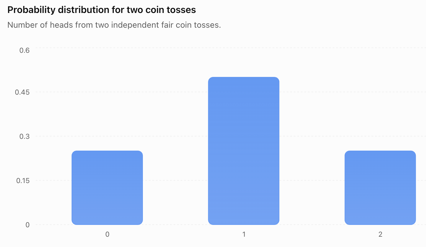
Expected Value of a Probability Model
The expected value describes the long-run average outcome of a random variable.
For a discrete random variable:
E(X) = Σ[x × P(X = x)]
The symbol Σ means to add the terms for all possible values of X.
Worked Example: Number of Heads
Using the previous model:
|
X |
P(X) |
X × P(X) |
|---|---|---|
|
0 |
0.25 |
0 |
|
1 |
0.50 |
0.50 |
|
2 |
0.25 |
0.50 |
Add:
E(X) = 0 + 0.50 + 0.50
E(X) = 1
The expected number of heads in two fair coin tosses is one.
This does not mean every experiment produces exactly one head.
It describes the average result over many repetitions.
Evaluating Model Assumptions
Every probability model relies on assumptions.
An assumption is a condition accepted as true for the purpose of constructing or using a model.
Assumptions simplify complicated situations and make mathematical analysis possible.
However, unrealistic assumptions can lead to misleading predictions.
Common Probability Assumptions
Independence
One event does not affect the probability of another.
Constant Probability
The probability of an event remains unchanged across trials.
Equal Likelihood
All outcomes have the same probability.
Random Sampling
Observations are selected using an appropriate random process.
Stable Conditions
The system behaves consistently over the period being modelled.
Appropriate Distribution
The selected probability distribution reasonably represents the data.
Example: Basketball Free Throws
Suppose a basketball player has a 75% probability of making a free throw.
A binomial model might assume:
-
Each shot has two outcomes: success or failure.
-
The number of shots is fixed.
-
Each shot is independent.
-
The probability of success remains 0.75.
In reality, performance may change because of fatigue, pressure, or confidence.
The binomial model may still be useful, but its assumptions should be considered.
Model Assumptions and Accuracy
A probability model can be mathematically correct while providing inaccurate predictions.
For example, suppose a factory's defect rate increases because a machine is wearing out.
A model assuming a constant 2% defect rate may underestimate future defects.
The calculations could be performed correctly, but the model would no longer describe the actual production process accurately.
Questions for Evaluating a Model
-
Are the possible outcomes correctly identified?
-
Are probabilities based on reliable information?
-
Are the events independent?
-
Does the probability remain constant?
-
Is the sample representative?
-
Does the selected distribution match the observed data?
-
Are important variables missing?
-
Do predictions agree with observations?
A useful model should be both mathematically valid and appropriate for the situation.
Comparing Competing Probability Models
Sometimes several probability models could describe the same situation.
We must determine which model is most appropriate.
Example: Customer Arrivals
Suppose a shop receives customers throughout the day.
We want to model the number of arrivals during a 10-minute interval.
Possible models include:
Binomial Model
This may be appropriate if there is a fixed number of potential customers, each independently deciding whether to arrive during the interval with the same probability.
Poisson Model
This may be appropriate if customers arrive independently at an approximately constant average rate.
Empirical Model
This uses observed customer counts without assuming a particular theoretical distribution.
Comparing the Models
|
Criterion |
Binomial |
Poisson |
Empirical |
|---|---|---|---|
|
Fixed number of trials |
Required |
Not required |
Not necessarily |
|
Constant probability or rate |
Constant success probability |
Constant event rate |
Not required |
|
Independence |
Required between trials |
Required by standard Poisson-process assumptions |
Depends on data |
|
Uses observed data |
Can estimate parameters |
Can estimate rate |
Directly |
|
Typical application |
Number of successes |
Number of arrivals |
Observed outcome frequencies |
The best model depends on the situation and available evidence.
Worked Example: Choosing a Probability Model
A call centre receives an average of four calls per minute.
We want to calculate the probability of receiving exactly six calls in one minute.
A Poisson distribution may be appropriate if calls arrive independently at a constant average rate.
Let:
X = number of calls per minute
λ = 4
Then:
X ~ Poisson(4)
The Poisson probability formula is:
P(X = k) = e^(−λ) × λᵏ/k!
Substitute:
P(X = 6) = e^(−4) × 4⁶/6!
= e^(−4) × 4096/720
P(X = 6) ≈ 0.1042
There is approximately a 10.42% probability of receiving exactly six calls in one minute under this model.
Evaluating the Model
The Poisson model may be unsuitable if:
-
Calls arrive in clusters.
-
The call rate changes significantly during the interval.
-
One call causes additional calls.
-
The arrival process is not independent.
The probability is conditional on the model assumptions being reasonable.

Comparing Theoretical Models with Observed Data
A useful way to evaluate a model is to compare its predictions with actual observations.
Suppose a model predicts the following probabilities for the number of customers arriving during a short interval.
|
Customers |
Model probability |
Expected count in 1,000 intervals |
Observed count |
|---|---|---|---|
|
0 |
0.10 |
100 |
95 |
|
1 |
0.25 |
250 |
260 |
|
2 |
0.35 |
350 |
340 |
|
3 |
0.20 |
200 |
205 |
|
4 or more |
0.10 |
100 |
100 |
|
Total |
1.00 |
1,000 |
1,000 |
The observed frequencies are reasonably close to the predicted frequencies.
However, differences remain because of random variation.
Evaluating the Fit
A model can be evaluated by considering:
-
Differences between predicted and observed frequencies.
-
Patterns in the errors.
-
Whether some outcomes occur more often than expected.
-
Whether the model remains accurate over time.
Formal statistical methods, such as goodness-of-fit tests, can provide additional evidence about model suitability.
Model Error and Uncertainty
Probability models involve different sources of uncertainty.
Random Variation
Even when a model is correct, actual outcomes vary randomly.
For example, a fair coin may produce seven heads in ten tosses.
Sampling Error
Probabilities estimated from samples may differ from population probabilities.
Measurement Error
Observations may contain inaccuracies.
Model Error
The mathematical model may fail to represent important features of the real system.
Parameter Uncertainty
The values used in the model, such as a success probability or event rate, may be estimated imperfectly.
Important Distinction
Increasing the sample size generally reduces sampling error.
However, it does not automatically correct an inappropriate probability model.
Solving Applied Probability Problems
Many practical probability problems involve several events or conditions.
The most important step is choosing an appropriate model.
Worked Example: Manufacturing Defects
A factory produces components with a 3% probability of being defective.
Suppose ten components are selected independently.
Find the probability that exactly two are defective.
Step 1: Select the Model
The number of defects follows a binomial distribution under the stated assumptions.
X ~ B(10, 0.03)
Step 2: Apply the Formula
P(X = k) = C(n,k) × pᵏ × (1 − p)^(n−k)
Substitute:
P(X = 2) = C(10,2) × 0.03² × 0.97⁸
Since:
C(10,2) = 45
P(X = 2) = 45 × 0.0009 × 0.97⁸
P(X = 2) ≈ 0.0317
There is approximately a 3.17% probability that exactly two of the ten components are defective.
Interpretation
This probability is valid if the defect probability remains constant and the selected components can reasonably be treated as independent.
Worked Example: Continuous Probability Model
Suppose a bus arrives at a uniformly random time between 0 and 12 minutes after a passenger reaches the bus stop.
Let:
X = waiting time
X ~ U(0, 12)
Find the probability that the passenger waits between 3 and 7 minutes.
Step 1: Determine the Interval Lengths
Total interval:
12 − 0 = 12 minutes
Favourable interval:
7 − 3 = 4 minutes
Step 2: Calculate the Probability
P(3 ≤ X ≤ 7) = 4/12
P(3 ≤ X ≤ 7) = 1/3 ≈ 0.3333
There is approximately a 33.33% probability that the passenger waits between three and seven minutes.
Model Evaluation
This assumes that arrival time is uniformly distributed across the interval.
If buses are more likely to arrive near particular times, the uniform model would be inappropriate.
Worked Example: Conditional Probability Model
Suppose a factory uses two machines.
Machine A produces 60% of components.
Machine B produces 40%.
The defect rates are:
-
Machine A: 2%.
-
Machine B: 5%.
Find the probability that a randomly selected component is defective.
Step 1: Define Events
A = component produced by Machine A
B = component produced by Machine B
D = component is defective
Step 2: Apply the Law of Total Probability
P(D) = P(D | A)P(A) + P(D | B)P(B)
Substitute:
P(D) = 0.02 × 0.60 + 0.05 × 0.40
= 0.012 + 0.020
P(D) = 0.032
There is a 3.2% probability that a randomly selected component is defective.
Why This Model Is Appropriate
The calculation accounts for both machines and their different production proportions.
Using a simple average of the two defect rates would be inappropriate because the machines produce different proportions of the total output.
Worked Example: Comparing Two Models
Suppose a company wants to estimate the number of defective products in a shipment.
Two possible models are proposed.
Model A: Binomial
Each product independently has a 4% probability of being defective.
Model B: Poisson
The number of defects is modelled using a Poisson distribution with mean 4 per 100 products.
For a shipment of 100 products:
Model A:
X ~ B(100, 0.04)
Model B:
X ~ Poisson(4)
Probability of No Defects
For the binomial model:
P(X = 0) = 0.96¹⁰⁰
≈ 0.0169
For the Poisson model:
P(X = 0) = e^(−4)
≈ 0.0183
The results are similar.
Interpretation
The Poisson model can approximate a binomial model when the number of trials is large and the success probability is small.
However, the approximation is not exact.
The binomial model may be preferable when the fixed number of trials and individual defect probability are known.
Using Simulation to Evaluate Models
Simulation can help evaluate a probability model by generating outcomes and comparing them with theoretical predictions.
For example, suppose a binomial model predicts:
P(success) = 0.6
A simulation can generate thousands of independent trials with a 60% success probability.
The resulting success proportion should generally be close to 0.6 when enough trials are performed.
Simulation Procedure
-
Define the probability model.
-
Generate random outcomes according to the model.
-
Repeat the experiment many times.
-
Calculate simulated probabilities.
-
Compare simulated results with theoretical predictions.
-
Investigate any substantial differences.
Important Limitation
A simulation that uses the same assumptions as the theoretical model mainly checks the calculation or implementation.
It does not prove that the model accurately describes the real world.
Real observations are needed to evaluate the model's practical validity.

Sensitivity Analysis
Sensitivity analysis investigates how changes in model assumptions or parameters affect the results.
Suppose a factory estimates a 3% defect probability.
However, the true defect probability may be between 2% and 5%.
For ten independent components, the probability of at least one defect is:
P(at least one defect) = 1 − (1 − p)¹⁰
Calculate this probability for different values of p.
|
Defect probability |
P(at least one defect) |
|---|---|
|
0.02 |
0.1829 |
|
0.03 |
0.2626 |
|
0.04 |
0.3352 |
|
0.05 |
0.4013 |
The probability of at least one defect changes substantially as the assumed defect rate increases.
Interpretation
The model's predictions are sensitive to the value of p.
This means that accurately estimating the defect rate is important.
Sensitivity analysis helps identify which assumptions have the greatest influence on model results.
Probability Models in Science
Probability models are widely used in scientific investigations.
Genetics
Probability can describe the likelihood of inheriting particular genetic combinations under specified inheritance models.
Ecology
Models can estimate population changes, species survival, or movement between habitats.
Chemistry
Probability models can describe random molecular behaviour and certain reaction processes.
Physics
Probability is important in radioactive decay, statistical mechanics, and quantum phenomena.
Environmental Science
Models can estimate rainfall, flooding, pollution exposure, and other uncertain environmental events.


Probability Models in Business and Engineering
Insurance
Insurance companies use probability models to estimate the frequency and cost of claims.
Manufacturing
Factories model defect rates, equipment failures, and product reliability.
Transportation
Probability models can estimate travel times, traffic delays, and vehicle arrivals.
Finance
Models can estimate uncertain returns, losses, and financial risks.
Project Management
Probability models can estimate completion times and the likelihood of meeting deadlines.
These applications often involve several uncertain variables, making model selection and evaluation especially important.
Communicating Probability Reasoning
A probability calculation is most useful when it is explained clearly.
A complete solution should communicate:
-
What is being investigated.
-
Which events or random variables are involved.
-
Which probability model is being used.
-
Why the model is appropriate.
-
Which assumptions are required.
-
How the calculation is performed.
-
What the result means in context.
-
What limitations may affect the conclusion.
Example of a Clear Probability Explanation
A factory produces components with a 5% probability of being defective.
Assuming ten components are selected independently and the defect probability remains constant, the number of defective components follows a binomial distribution.
The probability that all ten components are non-defective is:
P(X = 0) = 0.95¹⁰
≈ 0.5987
Therefore, there is approximately a 59.87% probability that none of the ten components is defective.
This result depends on the assumptions of independence and constant defect probability.
Why This Is Effective
The explanation identifies:
-
The situation.
-
The mathematical model.
-
The assumptions.
-
The calculation.
-
The interpretation.
It communicates both the numerical result and the reasoning behind it.
Evaluating Competing Models
When several models are available, compare them systematically.
Model Selection Criteria
Accuracy
How closely does the model match observed data?
Simplicity
Is the model unnecessarily complicated?
Assumptions
Are the assumptions realistic?
Interpretability
Can the model's predictions be explained clearly?
Data Requirements
Is enough reliable information available to estimate the parameters?
Predictive Performance
Does the model make accurate predictions on new observations?
Practical Usefulness
Does the model provide information that helps answer the original question?
The Balance Between Simplicity and Accuracy
A simple model may be easier to understand and apply.
A more complex model may capture additional details.
However, complexity does not automatically improve predictions.
The best model is one that represents the important features of the situation without unnecessary complication.
Common Mistakes
Selecting a distribution without checking its assumptions
Different distributions require different conditions.
Assuming all outcomes are equally likely
Many real-world outcomes have different probabilities.
Ignoring dependence between events
Dependent events require conditional probability calculations or other suitable models.
Confusing discrete and continuous variables
Counts and measurements often require different probability distributions.
Using a simple average when a weighted average is required
Groups contributing different proportions must be weighted appropriately.
Assuming a mathematically valid model is realistic
A model can satisfy probability rules while failing to represent real-world behaviour.
Ignoring sampling error
Probabilities estimated from samples contain uncertainty.
Confusing simulation accuracy with model validity
A simulation may reproduce the model accurately even when the model is inappropriate.
Comparing models using only one prediction
Models should be evaluated across relevant outcomes and observations.
Reporting probabilities without context
A numerical answer should be interpreted in terms of the original problem.
Failing to state assumptions
Assumptions are essential for understanding when a probability calculation is valid.
Key Terms
-
Probability Model: A mathematical representation of possible outcomes and their probabilities.
-
Random Experiment: A process whose outcome is uncertain.
-
Sample Space: The set of all possible outcomes of an experiment.
-
Event: A collection of outcomes within a sample space.
-
Random Variable: A numerical variable whose value depends on a random outcome.
-
Discrete Random Variable: A random variable with a finite or countably infinite set of possible values.
-
Continuous Random Variable: A random variable that can take any real value within an interval or collection of intervals.
-
Probability Distribution: A description of how probability is assigned to possible values.
-
Theoretical Probability: A probability calculated using mathematical assumptions.
-
Empirical Probability: A probability estimated using observed data.
-
Simulation: A process that imitates uncertain outcomes using a mathematical or computational model.
-
Bernoulli Distribution: A probability model for a single success-or-failure trial.
-
Binomial Distribution: A probability model for the number of successes in a fixed number of independent trials.
-
Geometric Distribution: A probability model for the number of trials until the first success.
-
Poisson Distribution: A probability model for counts of events occurring at a constant average rate under specified assumptions.
-
Uniform Distribution: A distribution with equally likely discrete outcomes or constant density over a continuous interval.
-
Normal Distribution: A symmetrical, bell-shaped continuous probability distribution.
-
Exponential Distribution: A continuous distribution commonly used to model waiting times in a Poisson process.
-
Expected Value: The long-run average outcome of a random variable.
-
Variance: A measure of how widely values are spread around the mean.
-
Model Assumption: A condition accepted when constructing or applying a model.
-
Independence: A relationship in which one event does not change the probability of another.
-
Conditional Probability: The probability of an event given that another event has occurred.
-
Parameter: A numerical value describing a probability distribution.
-
Model Error: Error caused by differences between the mathematical model and the real system.
-
Sampling Error: Variation caused by estimating quantities from a sample.
-
Goodness of Fit: A measure of how closely a model agrees with observed data.
-
Sensitivity Analysis: An investigation of how model results change when assumptions or parameters change.
-
Predictive Performance: How accurately a model predicts new outcomes.
-
Probability Reasoning: The use of mathematical evidence and logical explanations to analyse uncertainty.
Key Takeaways
-
Probability models describe uncertain situations using possible outcomes and assigned probabilities.
-
A valid probability model assigns probabilities between 0 and 1.
-
The probabilities of mutually exclusive, exhaustive outcomes must add to 1.
-
Constructing a probability model requires defining the experiment, outcomes, probabilities, and assumptions.
-
Discrete probability models describe countable outcomes, while continuous models describe values across intervals.
-
Different probability distributions are appropriate for different situations.
-
Bernoulli, binomial, geometric, and Poisson distributions are common discrete models.
-
Uniform, normal, and exponential distributions are important continuous models.
-
Expected value describes the long-run average outcome of a probability model.
-
Every probability model depends on assumptions.
-
Independence, constant probabilities, random sampling, and distribution shape are common assumptions.
-
A mathematically correct model may still produce inaccurate real-world predictions.
-
Competing models should be compared using assumptions, accuracy, simplicity, and predictive performance.
-
Observed data can be used to evaluate how well a model fits a situation.
-
Simulation provides a useful way to investigate complex probability models.
-
Sensitivity analysis shows how predictions change when model parameters change.
-
Probability models are widely used in science, manufacturing, finance, transportation, and engineering.
-
Clear probability reasoning includes the model, assumptions, calculations, interpretation, and limitations.
Check Your Understanding
Recall and Understanding
-
Define a probability model and explain its purpose.
-
State the two fundamental requirements of a valid probability model.
-
Explain the difference between discrete and continuous probability models.
-
Identify three assumptions commonly used in probability modelling.
-
Explain why a mathematically correct model may still produce inaccurate predictions.
Application
-
A fair die is rolled once. Construct a probability model for the outcome and verify that the probabilities add to 1.
-
Two fair coins are tossed. Construct a probability distribution for the number of heads and calculate its expected value.
-
A factory produces components with a 4% probability of being defective. Assuming independence, calculate the probability that exactly one of five components is defective.
-
A call centre receives an average of three calls per minute. Assuming a Poisson model is appropriate, calculate the probability of receiving exactly two calls in one minute.
-
A bus arrives uniformly between 0 and 15 minutes after a passenger begins waiting. Calculate the probability that the waiting time is between 5 and 10 minutes.
Analysis and Challenge
-
A basketball player makes 80% of free throws. Explain the assumptions required to model the number of successes in ten attempts using a binomial distribution.
-
A factory uses two machines. Machine A produces 70% of components with a 2% defect rate, while Machine B produces 30% with a 6% defect rate. Calculate the overall probability that a component is defective.
-
A company is comparing a binomial model and a Poisson model for the number of defects in a shipment. Explain when each model would be appropriate and identify the limitations of the Poisson approximation.
-
A probability model predicts that 10% of products will be defective, but observed data show that 18% are defective. Suggest possible reasons for the difference and explain how the model could be improved.
-
Design a probability model for a real-world situation of your choice. Define the random variable, select an appropriate distribution, state the assumptions, demonstrate one probability calculation, and explain how you would evaluate the model's accuracy.
Final Summary
Probability models provide a structured mathematical approach to understanding and predicting uncertain outcomes.
Constructing a model involves identifying possible outcomes, assigning probabilities, selecting suitable distributions, and stating the assumptions required.
Different models are appropriate for different situations, and no single distribution can describe every random process.
Evaluating probability models requires comparing predictions with observations, examining assumptions, and considering uncertainty and model limitations.
By selecting appropriate models, performing calculations, and communicating reasoning clearly, students can apply probability to practical problems in science, engineering, business, and everyday life.
The most important principle is that a probability model is useful not simply because it produces a numerical answer, but because its assumptions and predictions provide a reasonable representation of the situation being studied.