Simulation and Monte Carlo Methods

Introduction to Simulation and Monte Carlo Methods

Many real-world situations involve uncertainty. Sometimes probabilities can be calculated exactly using mathematical formulas, but other problems are too complicated for a simple theoretical solution.

For example:

• What is the probability of winning a particular board game?

• How likely is a project to finish before its deadline?

• What is the chance that a machine will fail during a given period?

• How often will a particular combination of dice rolls occur?

• How accurately can we estimate an area using randomly generated points?

One approach is to create a mathematical or computer-based model and repeat an experiment many times.

This process is called simulation.

A particularly important simulation technique is the Monte Carlo method, which uses random sampling and repeated trials to estimate probabilities or numerical quantities.

Simulation is widely used in science, engineering, finance, medicine, weather forecasting, computer science, and probability research.

What Is a Simulation?

A simulation is a model that imitates the behaviour of a real or hypothetical system.

Instead of observing the actual system repeatedly, we reproduce its important features using mathematical rules, physical objects, or computer programs.

A simulation might involve:

• Tossing coins.

• Rolling dice.

• Drawing numbered cards.

• Generating random numbers.

• Using spreadsheet formulas.

• Running a computer program.

Example: Simulating Coin Tosses

Suppose we want to estimate the probability of obtaining heads when tossing a fair coin.

We could toss a real coin 100 times and record the outcomes.

Alternatively, we could use a random number generator:

• Generate 0 to represent tails.

• Generate 1 to represent heads.

Repeating this process many times produces a simulated coin-toss experiment.

The proportion of heads can then be compared with the theoretical probability of 0.5.

Theoretical and Experimental Probability

Theoretical Probability

Theoretical probability is calculated using a mathematical model.

For equally likely outcomes:

P(E) = Number of favourable outcomes / Total number of possible outcomes

For example, the probability of rolling a 6 on a fair die is:

P(6) = 1/6

≈ 0.1667

Experimental Probability

Experimental probability is estimated from observations or repeated trials.

Experimental probability = Number of times event occurs / Total number of trials

For example, suppose a die is rolled 120 times and a 6 appears 23 times.

Experimental probability:

P(6) ≈ 23/120

P(6) ≈ 0.1917

This differs from the theoretical probability of approximately 0.1667.

The difference is expected because random experiments produce variation.

What Is a Monte Carlo Simulation?

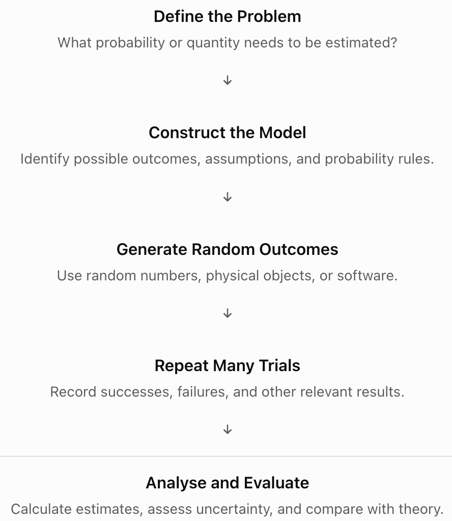
A Monte Carlo simulation is a method that uses random sampling to investigate a mathematical or real-world problem.

The method generally involves:

1. Defining a problem.

2. Creating a mathematical model.

3. Generating random inputs.

4. Repeating the experiment many times.

5. Recording the outcomes.

6. Using the results to estimate probabilities or other quantities.

The name Monte Carlo refers to the famous casino district in Monaco, reflecting the importance of randomness in the method.

Monte Carlo methods are especially useful when exact calculations are difficult or when a system contains several uncertain variables.

The Monte Carlo Simulation Process

Performing a Simple Coin-Toss Simulation

Suppose we want to estimate the probability of obtaining heads on a fair coin.

Step 1: Define the Outcomes

The possible outcomes are:

• Heads

• Tails

The theoretical probabilities are:

P(Heads) = 0.5

P(Tails) = 0.5

Step 2: Simulate the Experiment

Generate random outcomes representing heads or tails.

Step 3: Record the Results

Suppose a simulation produces the following illustrative results:

These are example results, not guaranteed outcomes of a simulation.

Step 4: Compare With Theory

The theoretical probability is:

P(Heads) = 0.5

As the number of trials increases, the experimental probability often becomes closer to 0.5.

However, random fluctuations remain possible.

Interactive Coin-Toss Simulation

Try simulating a fair coin below. Each batch adds new trials, allowing you to observe how the estimated probability changes.

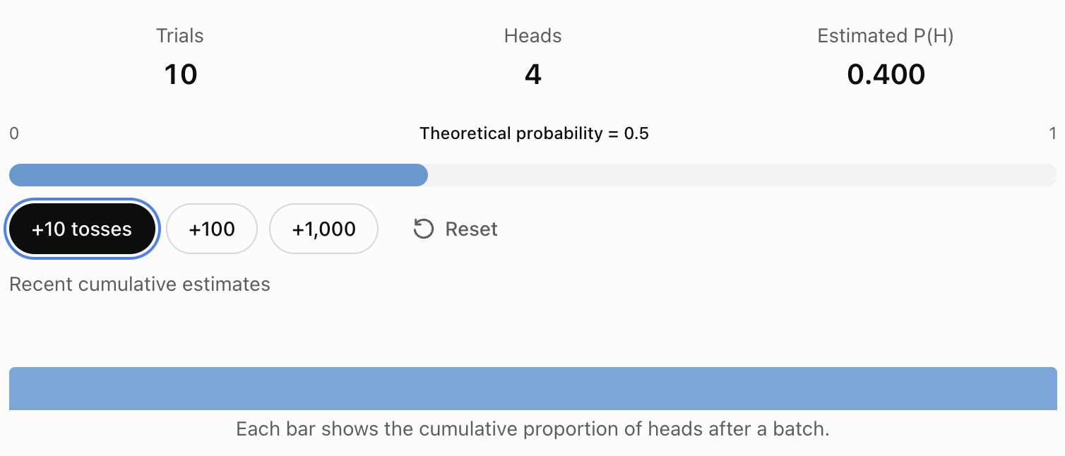
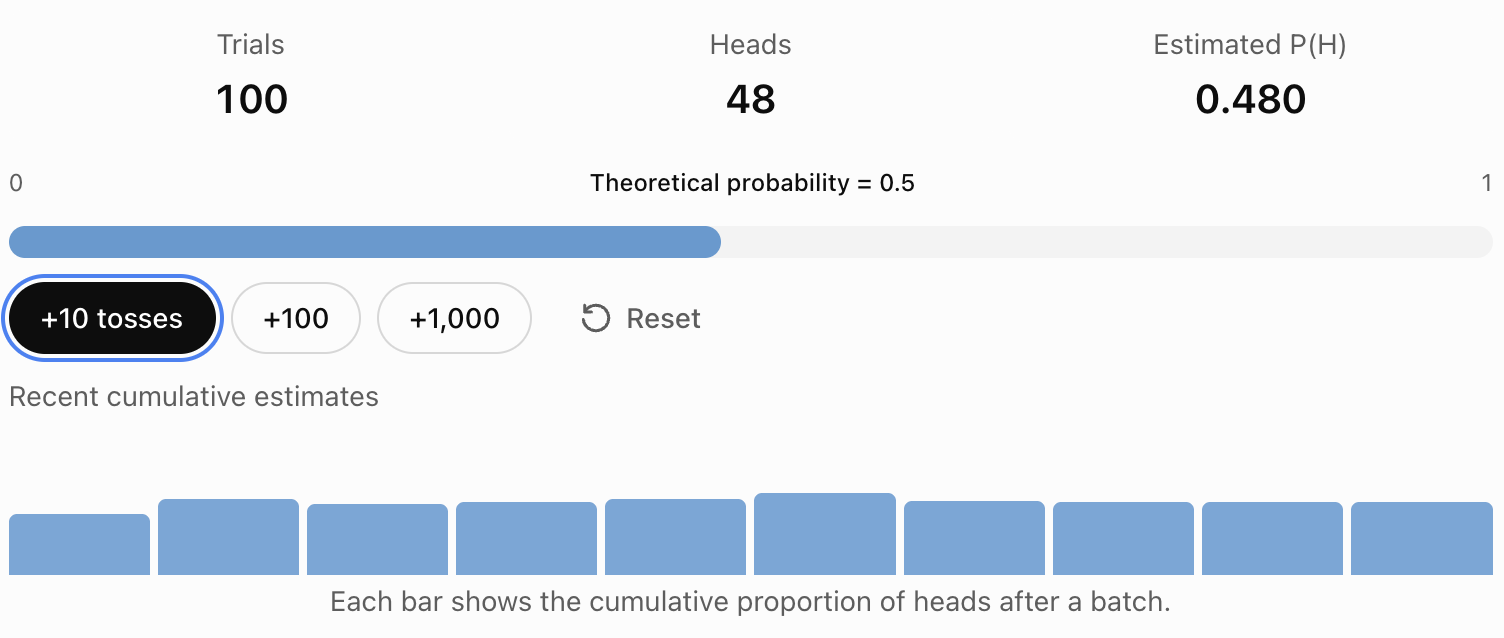
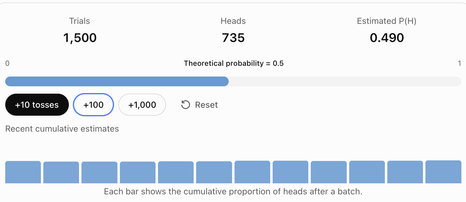
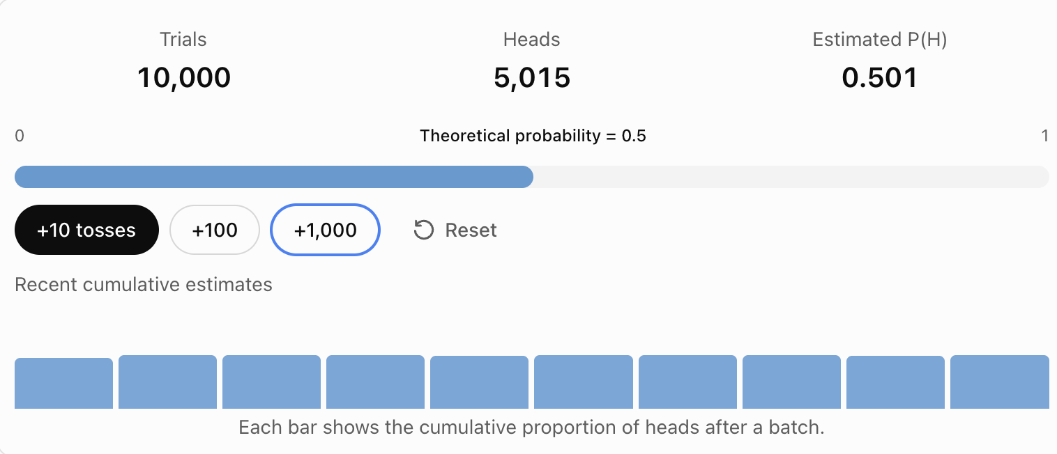
The estimate should generally become more stable as the number of tosses increases, although it will not necessarily move closer to 0.5 after every batch.

The Law of Large Numbers

The Law of Large Numbers states that, under appropriate conditions, the average result of many independent repetitions approaches the expected value as the number of trials increases.

For a fair coin:

Expected proportion of heads = 0.5

As more tosses are performed, the observed proportion tends to approach 0.5.

Important Distinction

The Law of Large Numbers does not mean that the number of heads and tails must become equal.

For example, after 10,000 tosses, it is possible to have:

• 5,080 heads.

• 4,920 tails.

The difference is 160 tosses.

However, the proportion of heads is:

5,080/10,000 = 0.508

This is relatively close to the theoretical probability of 0.5.

The absolute difference between the counts may increase even while the relative frequencies become more stable.

Simulating Dice Rolls

Suppose we want to estimate the probability of rolling a total of 7 with two fair dice.

Theoretical Probability

Each die has six possible outcomes.

The total number of equally likely ordered outcomes is:

6 × 6 = 36

The combinations producing a total of 7 are:

(1,6), (2,5), (3,4), (4,3), (5,2), (6,1)

There are six favourable outcomes.

Therefore:

P(sum = 7) = 6/36

P(sum = 7) = 1/6 ≈ 0.1667

Monte Carlo Method

A simulation would:

1. Generate a random integer from 1 to 6.

2. Generate a second independent random integer from 1 to 6.

3. Add the two values.

4. Record whether the sum equals 7.

5. Repeat thousands of times.

Suppose the simulation produces 1,681 successes in 10,000 trials.

Experimental probability:

P(sum = 7) ≈ 1681/10000

P(sum = 7) ≈ 0.1681

The simulated result is close to the theoretical probability of approximately 0.1667.

Simulating Events with Unequal Probabilities

Not all simulations involve equally likely outcomes.

Suppose a basketball player has a 70% probability of making a free throw.

We can simulate each attempt using a random number between 0 and 1.

Define:

• Random number below 0.70 → successful shot.

• Random number at least 0.70 → missed shot.

If the random number generator produces values uniformly between 0 and 1, this gives the required success probability.

Example

Suppose the generated random numbers are:

0.24, 0.83, 0.65, 0.11, 0.92

The corresponding outcomes are:

Success, Miss, Success, Success, Miss

Three successes occur in five attempts.

Experimental success rate:

3/5 = 0.60

Although the theoretical success probability is 0.70, a small sample can produce a different result.

Monte Carlo Simulation of a Binomial Experiment

Suppose a basketball player makes each independent free throw with probability 0.7.

The player attempts ten shots.

We want to estimate:

P(exactly 7 successful shots)

Theoretical Calculation

The number of successes follows a binomial distribution:

X ~ B(10, 0.7)

The probability is:

P(X = 7) = C(10,7) × 0.7⁷ × 0.3³

Since:

C(10,7) = 120

P(X = 7) = 120 × 0.7⁷ × 0.3³

P(X = 7) ≈ 0.2668

Simulation Method

One simulated experiment consists of ten independent free throws.

For each experiment:

• Generate ten random numbers.

• Count how many are below 0.7.

• Record whether exactly seven successes occurred.

Repeat the experiment many times.

If exactly seven successes occur in 2,659 of 10,000 simulated experiments:

Estimated probability:

2659/10000 = 0.2659

This is close to the theoretical value of approximately 0.2668.

Estimating Pi Using Monte Carlo Methods

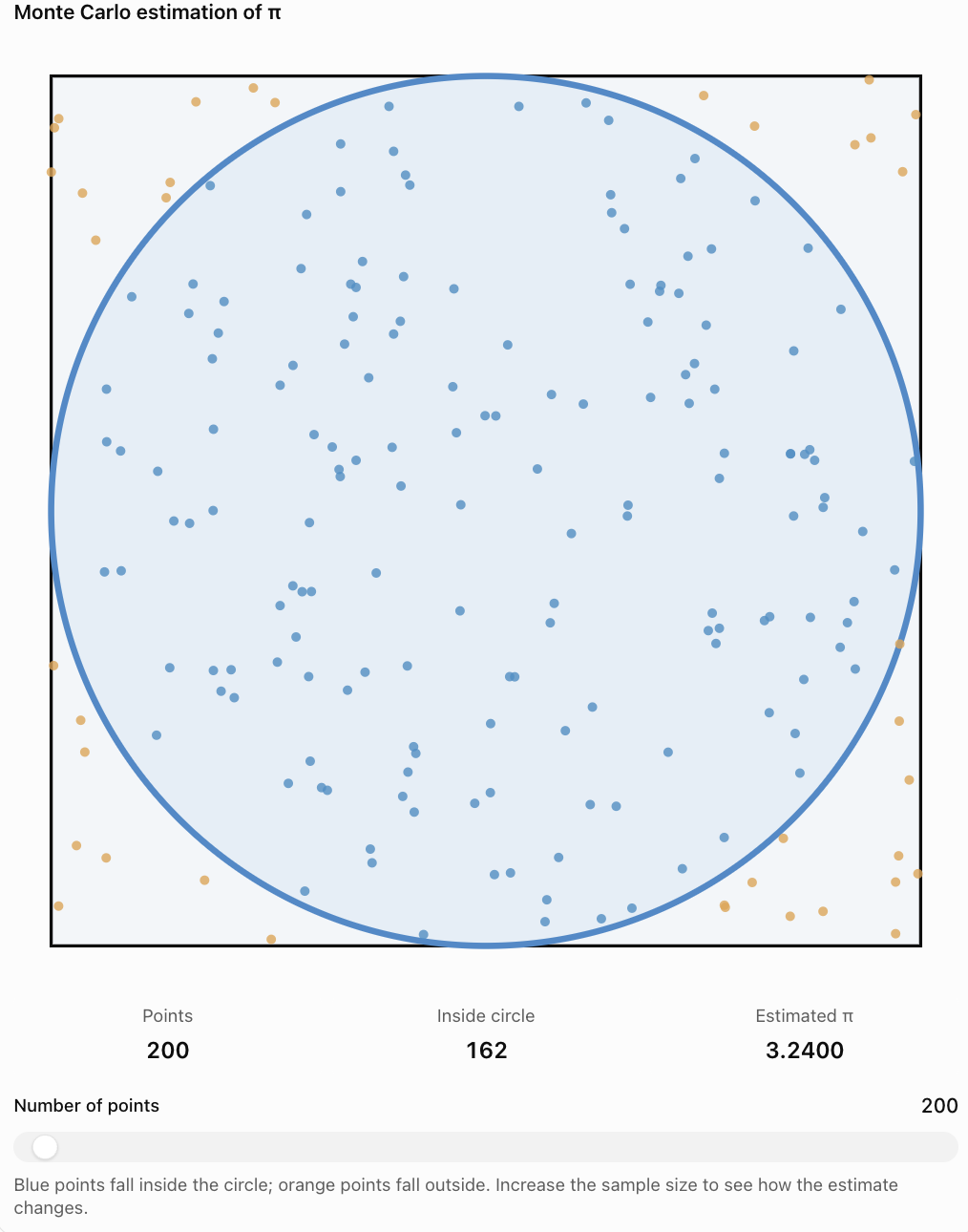
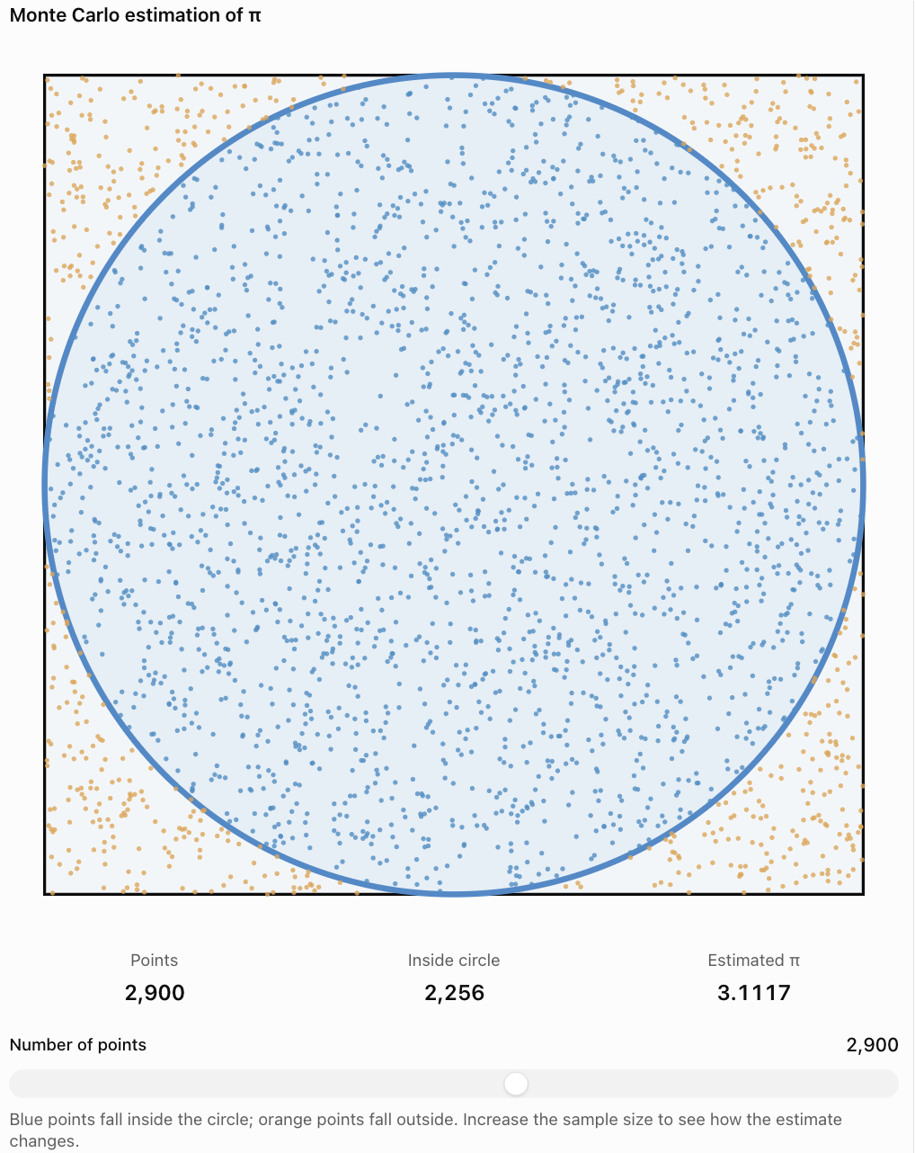
One famous application of Monte Carlo simulation is estimating the value of π.

Consider a square with side length 2.

Inside the square is a circle with radius 1.

Area of the Square

Area = 2 × 2

Area = 4

Area of the Circle

Area = πr²

Since r = 1:

Area = π

Ratio of Areas

Circle area / Square area = π/4

Therefore:

π = 4 × (Circle area / Square area)

Monte Carlo Method

Generate random points uniformly inside the square.

Count how many fall inside the circle.

The proportion of points inside the circle estimates the ratio of the areas.

Therefore:

π ≈ 4 × (Points inside circle / Total points)

Example

Suppose 10,000 points are generated.

7,860 fall inside the circle.

Estimated π:

π ≈ 4 × (7860/10000)

= 4 × 0.786

π ≈ 3.144

This is close to the actual value:

π ≈ 3.14159

Comparing Theoretical and Simulated Results

Simulation estimates should be compared with theoretical values whenever those values are available.

Example: Rolling a Six

The theoretical probability of rolling a 6 on a fair die is:

P(6) = 1/6 ≈ 0.1667

Suppose a simulation produces the following results:

These are illustrative results.

Absolute Error

The absolute error measures the difference between the simulated estimate and theoretical value.

Absolute error = |Simulated probability − Theoretical probability|

For 1,000 trials:

Absolute error = |0.1740 − 0.1667|

≈ 0.0073

A smaller absolute error indicates that the simulation estimate is closer to the theoretical probability.

However, increasing the number of trials does not guarantee that every individual estimate will be closer than the previous one.

Evaluating Simulation Accuracy

Simulation results are affected by several factors.

Number of Trials

Larger simulations generally produce more stable estimates.

Small samples are more strongly affected by random fluctuations.

Quality of the Random Number Generator

A simulation depends on the quality of its random inputs.

Poor random-number generation can introduce patterns or bias.

Model Assumptions

A simulation may produce very precise results while still being inaccurate if the underlying model is unrealistic.

For example, a basketball simulation assuming a constant 70% success probability may ignore fatigue, pressure, and changing conditions.

Independence

Many probability simulations assume that trials are independent.

If events influence one another, the model must account for that dependence.

Correct Implementation

Programming errors, incorrect formulas, or improper recording of outcomes can produce misleading results.

Reproducibility

Computer simulations often use pseudorandom number generators.

A fixed random seed can allow the same sequence of random numbers to be reproduced, which is useful for checking results.

Sampling Error and Standard Error

A Monte Carlo estimate is subject to sampling error because it is calculated using a finite number of random trials.

Suppose an event has true probability p.

After n independent trials, the estimated probability is:

p̂ = Number of successes / n

The approximate standard error of this estimate is:

SE = √[p(1 − p)/n]

Because the true value of p is often unknown, it can be estimated using:

Estimated SE = √[p̂(1 − p̂)/n]

Worked Example

Suppose a simulation estimates a probability of:

p̂ = 0.4

using:

n = 1,000 trials

Estimated standard error:

SE ≈ √[(0.4 × 0.6)/1000]

= √0.00024

SE ≈ 0.0155

The estimated standard error is approximately 0.0155, or 1.55 percentage points.

Interpretation

The standard error describes the typical variation in the simulated estimate across repeated simulations of the same size.

It is not the difference between the estimate and the true probability for one particular run.

Confidence Intervals for Simulated Probabilities

A confidence interval provides a range of plausible values for an unknown probability.

For a sufficiently large sample, an approximate 95% confidence interval can be calculated as:

p̂ ± 1.96 × SE

Worked Example

Suppose:

p̂ = 0.4

SE ≈ 0.0155

Calculate:

1.96 × 0.0155 ≈ 0.0304

Lower boundary:

0.4 − 0.0304 = 0.3696

Upper boundary:

0.4 + 0.0304 = 0.4304

Therefore, an approximate 95% confidence interval is:

0.370 to 0.430

This suggests that the true probability is plausibly between approximately 37.0% and 43.0%, under the assumptions of the method.

This simple interval is an approximation and may perform poorly for very small samples or probabilities close to 0 or 1.

How Simulation Accuracy Changes with Sample Size

The standard error of a probability estimate is proportional to:

1/√n

This means that simulation accuracy improves relatively slowly as the number of trials increases.

For example:

• Doubling the number of trials reduces standard error by a factor of √2.

• Increasing trials by a factor of 4 approximately halves standard error.

• Increasing trials by a factor of 100 reduces standard error by a factor of 10.

Example

Suppose a simulation uses 1,000 trials.

To reduce the standard error to half its original size, approximately:

4,000 trials

are required.

This is an important consideration when deciding how many trials to perform.

Monte Carlo Simulation in Spreadsheets

Spreadsheet software can be used to perform simple Monte Carlo simulations.

For example, in Excel or Google Sheets:

Simulating a Coin Toss

Use:

=IF(RAND()<0.5,"Heads","Tails")

This generates either Heads or Tails with equal probability.

Simulating a Die Roll

Use:

=RANDBETWEEN(1,6)

This generates a random integer between 1 and 6.

Simulating a 70% Success Probability

Use:

=IF(RAND()<0.7,1,0)

A result of 1 represents success.

A result of 0 represents failure.

Estimating Probability

If the simulated results are recorded in cells A2 to A1001, with successes represented by 1:

=AVERAGE(A2:A1001)

This calculates the proportion of successful trials.

Important Note

Spreadsheet random functions may recalculate when the worksheet changes.

To preserve simulation results, copy the generated values and paste them as fixed values when needed.

Practical Application: Manufacturing Quality Control

Suppose a factory produces components with a 3% probability of being defective.

A shipment contains 100 components.

The factory wants to estimate the probability that more than five components are defective.

Simulation Model

For each component:

• Generate a random number between 0 and 1.

• If the number is below 0.03, record a defect.

• Otherwise, record a non-defective component.

Repeat this process for 100 components.

Count the number of defects.

One complete set of 100 components represents one simulated shipment.

Repeating the Simulation

Repeat the shipment simulation 10,000 times.

Suppose 790 simulated shipments contain more than five defective components.

Estimated probability:

P(more than 5 defects) ≈ 790/10000

= 0.079

The estimated probability is 7.9%.

Interpretation

The simulation suggests that approximately 7.9% of shipments may contain more than five defective components under the assumed model.

The result can help the company assess quality-control risks.

Practical Application: Project Completion Times

Suppose a project has three stages.

Each stage has an uncertain completion time.

For a simplified model, assume each stage's duration is independently and uniformly distributed between its minimum and maximum.

Simulation Procedure

For each simulated project:

1. Generate a random planning duration.

2. Generate a random development duration.

3. Generate a random testing duration.

4. Add the three durations.

5. Record whether the project finishes within 15 days.

Repeat thousands of times.

Example

Suppose 10,000 simulations are performed.

8,200 finish within 15 days.

Estimated probability:

P(completion within 15 days) ≈ 8200/10000

= 0.82

The simulation estimates an 82% probability of meeting the deadline.

This is an illustrative result, not a calculated prediction for a real project.

Limitations

Actual project stages may not have uniform durations or be independent.

For example, delays in development may increase testing time.

A more realistic simulation would need to account for these relationships.

Practical Application: Environmental Science

Monte Carlo methods can help scientists study uncertain environmental processes.

Examples include:

• Rainfall variability.

• River flooding.

• Population growth.

• Pollution dispersion.

• Forest-fire risk.

• Climate-related uncertainty.

Example: Rainfall

Suppose daily rainfall is modelled using a probability distribution.

A simulation can generate thousands of possible rainfall sequences.

Researchers can then estimate the probability of events such as:

• Rainfall exceeding a threshold.

• Several consecutive dry days.

• Extremely wet months.

• Water-storage shortages.

The quality of the predictions depends on the accuracy of the rainfall model and its assumptions.

Practical Application: Financial Risk

Monte Carlo simulations are frequently used to study financial uncertainty.

For example, an investment portfolio may experience different returns depending on market conditions.

A simulation can generate possible sequences of returns and estimate:

• Possible future portfolio values.

• Probability of losses.

• Range of outcomes.

• Risk associated with different assumptions.

However, financial simulations are only as reliable as the models used.

Real markets may experience extreme events, changing relationships, and unexpected behaviour that simplified models do not capture.

Simulation Versus Exact Probability

Simulation is especially useful when exact calculations are difficult.

However, it is not always the best method.

Exact Probability Methods

Advantages:

• Produce mathematically exact results when the model is known.

• Do not involve sampling error.

• Often efficient for simple problems.

Limitations:

• Can become complicated for large systems.

• May require advanced mathematical techniques.

Monte Carlo Methods

Advantages:

• Can handle complicated models.

• Flexible and adaptable.

• Useful when exact solutions are unavailable.

• Can incorporate multiple uncertain variables.

Limitations:

• Produce estimates rather than exact answers.

• Require many trials for high precision.

• Depend on random-number quality and model assumptions.

• Can be computationally expensive.

Comparison

Common Mistakes

Assuming simulated results must equal theoretical probabilities

Random variation causes simulated estimates to differ from theoretical values.

Using too few trials

Small samples can produce unstable probability estimates.

Assuming more trials eliminate all error

Larger samples reduce sampling error but do not remove model bias or programming errors.

Confusing experimental probability with theoretical probability

Experimental probability is based on observed outcomes, while theoretical probability comes from a mathematical model.

Assuming every random-number generator is perfectly random

Computer-generated random numbers are generally pseudorandom and depend on the algorithm used.

Ignoring independence assumptions

If trials are dependent, the simulation must account for those relationships.

Using an unrealistic model

A simulation can produce precise results that do not accurately represent reality.

Confusing absolute error with standard error

Absolute error compares an estimate with a known value. Standard error describes the variability of an estimator across repeated samples.

Assuming confidence intervals guarantee the true value lies inside

A 95% confidence interval method has approximately 95% long-run coverage under its assumptions; it does not guarantee that every interval contains the true value.

Failing to check simulation results

Simulation outputs should be tested against theoretical results or known cases whenever possible.

Key Terms

• Simulation: A model that imitates the behaviour of a real or hypothetical system.

• Monte Carlo Method: A technique using random sampling and repeated trials to estimate probabilities or numerical quantities.

• Random Sampling: Selecting values or outcomes according to a specified probability model.

• Random Number Generator: A device or algorithm that produces values used to simulate randomness.

• Pseudorandom Number: A computer-generated value produced by a deterministic algorithm designed to imitate randomness.

• Random Seed: An initial value used to generate a reproducible pseudorandom sequence.

• Trial: One repetition of a random experiment.

• Simulation Run: One execution of a simulated experiment or model.

• Theoretical Probability: A probability calculated mathematically from a model.

• Experimental Probability: A probability estimated from observed or simulated outcomes.

• Relative Frequency: The proportion of trials in which an event occurs.

• Law of Large Numbers: A principle stating that averages from many suitable independent trials approach their expected value.

• Sampling Error: Variation arising because an estimate is based on a finite random sample.

• Absolute Error: The absolute difference between an estimate and a reference value.

• Standard Error: A measure of the typical variation of an estimator across repeated samples.

• Confidence Interval: A range constructed using a method designed to contain an unknown parameter at a specified long-run rate.

• Probability Model: A mathematical representation of uncertain outcomes.

• Model Assumption: A condition accepted as part of a mathematical representation.

• Model Bias: Systematic error caused by an inappropriate or inaccurate model.

• Simulation Accuracy: How closely simulation results estimate the intended quantity.

• Simulation Precision: How consistently repeated simulations produce similar estimates.

• Convergence: The tendency of an estimate to approach a target value as the number of trials increases.

• Binomial Experiment: A fixed number of independent trials with two possible outcomes and constant success probability.

• Uniform Distribution: A probability distribution in which equal-length intervals have equal probabilities.

• Stochastic Model: A mathematical model involving randomness.

• Risk Analysis: The process of studying possible uncertain outcomes and their consequences.

Key Takeaways

• Simulation uses models to imitate uncertain processes or experiments.

• Monte Carlo methods use random sampling and repeated trials to estimate probabilities and other quantities.

• Simulations can be performed using physical objects, spreadsheets, or computer programs.

• Theoretical probability is calculated mathematically, while experimental probability is estimated from observations.

• A Monte Carlo simulation requires a clearly defined model, random inputs, repeated trials, and analysis of results.

• Increasing the number of trials generally improves the stability of simulation estimates.

• The Law of Large Numbers explains why relative frequencies tend to approach theoretical probabilities.

• Simulated results may differ from theoretical values because of random variation.

• Monte Carlo methods can estimate probabilities involving dice, coins, manufacturing defects, and many other systems.

• Random points inside geometric shapes can be used to estimate areas and mathematical constants such as π.

• Absolute error measures the difference between an estimate and a known value.

• Standard error describes the typical variation of an estimate across repeated simulations.

• Standard error generally decreases in proportion to 1/√n.

• Increasing simulation trials by a factor of four approximately halves standard error.

• Confidence intervals can help describe uncertainty in simulated probability estimates.

• A large simulation does not guarantee accuracy if the underlying model is unrealistic.

• Model assumptions, independence, random-number quality, and implementation must all be evaluated.

• Monte Carlo methods are useful in science, engineering, manufacturing, environmental modelling, finance, and decision-making.

Check Your Understanding

Recall and Understanding

1. Define simulation and explain its purpose.

2. What is a Monte Carlo simulation?

3. Explain the difference between theoretical probability and experimental probability.

4. State the Law of Large Numbers and explain its importance in simulation.

5. Identify three factors that affect the accuracy of a Monte Carlo simulation.

Application

6. A fair coin is tossed 200 times and heads appears 112 times. Calculate the experimental probability of heads and compare it with the theoretical probability.

7. A fair die is rolled 600 times and a 6 appears 92 times. Calculate the experimental probability and absolute error.

8. A simulation generates 10,000 random points inside a square. Of these, 7,850 fall inside an inscribed circle. Estimate π.

9. A basketball player has a 75% probability of making each free throw. Describe how to simulate 100 free throws using random numbers between 0 and 1.

10. A simulation estimates a probability of 0.35 using 2,000 independent trials. Calculate the approximate standard error.

Analysis and Challenge

11. Explain why a simulation using 10,000 trials is generally more reliable than one using 100 trials, but not guaranteed to produce a more accurate result in every run.

12. A factory produces components with a 4% probability of being defective. Design a Monte Carlo simulation to estimate the probability that more than three components are defective in a shipment of 50.

13. A project has three stages with uncertain durations. Explain how a Monte Carlo simulation could estimate the probability of completing the project before a deadline.

14. A simulation estimates a probability of 0.42 using 5,000 trials. Calculate an approximate 95% confidence interval and interpret it.

15. A simulation produces highly consistent results across repeated runs, but the predictions do not match real-world observations. Explain why this might happen and suggest improvements to the model.

Final Summary

Simulation and Monte Carlo methods provide powerful techniques for investigating uncertainty through repeated random experiments.

Instead of relying only on theoretical calculations, simulations generate many possible outcomes and use their relative frequencies to estimate probabilities.

The Law of Large Numbers explains why estimates generally become more stable as the number of trials increases.

However, simulation accuracy depends not only on sample size but also on the quality of the random-number generator, the correctness of the calculations, and the assumptions of the mathematical model.

By comparing theoretical and simulated results, calculating errors, and evaluating uncertainty, students can develop a deeper understanding of probability and statistical modelling.

Monte Carlo methods are especially valuable when studying complex systems where exact mathematical solutions are difficult or impractical.