Markov Processes

Introduction to Markov Processes

Many real-world situations involve systems that change over time. The changes are not always predictable, but the probabilities of different outcomes can often be estimated.

Consider the following situations:

• Tomorrow's weather may depend on today's weather.

• A customer may continue using a product or switch to another brand.

• A machine may remain operational or develop a fault.

• An animal may move between different habitats.

• A student may progress between different levels of understanding.

These situations can be studied using Markov processes.

A Markov process is a mathematical model describing a system that moves between different states according to probabilities.

The defining feature is that the probability of the next state depends on the current state, rather than the complete history of previous states.

This is called the Markov property.

Markov models are widely used in mathematics, science, economics, computing, engineering, and environmental research.

Understanding Stochastic Processes

A stochastic process is a mathematical model describing a system that changes over time in a way that involves randomness.

The word stochastic means that chance or probability influences the outcomes.

For example, consider the weather over several days.

The weather may be:

• Sunny

• Cloudy

• Rainy

The weather tomorrow is uncertain, even when today's weather is known.

However, past observations may help us estimate the probability of each possible outcome.

A stochastic process describes how these uncertain changes occur.

Deterministic Versus Stochastic Systems

A deterministic system produces an outcome that is completely determined by its initial conditions and governing rules.

A stochastic system includes uncertainty, so the same current conditions can lead to different outcomes.

Markov processes are a particular type of stochastic process.

The Markov Property

The central idea of a Markov process is that the future depends on the present state, not on the full history of previous states.

This is sometimes called the memoryless property.

For a sequence of states X₀, X₁, X₂, ...:

P(Xₙ₊₁ = j | Xₙ = i, earlier states) = P(Xₙ₊₁ = j | Xₙ = i)

This means that once the current state is known, earlier states provide no additional information about the probability of the next state.

Example: Weather

Suppose a simplified weather model contains two states:

• Sunny

• Rainy

If today is sunny, the probability of tomorrow being rainy is 0.3.

In a Markov model, this probability remains 0.3 regardless of whether yesterday was sunny or rainy.

The model uses today's weather to predict tomorrow's weather.

Important Limitation

Real weather depends on many variables, including atmospheric pressure, temperature, humidity, and wind.

A simple two-state Markov model is therefore an approximation.

Its usefulness depends on whether the chosen states contain enough information to make reasonable predictions.

States in a Markov Process

A state describes the condition of a system at a particular time.

Examples include:

A Markov model requires a clearly defined set of states.

Important Requirements

The states should be:

• Clearly defined.

• Mutually exclusive at a given observation time.

• Sufficient to describe the modelled system.

• Appropriate for the question being investigated.

For example, if weather states are defined as sunny and rainy, the model must specify how cloudy conditions are classified.

Otherwise, the states may not cover all possible outcomes.

Transition Probabilities

A transition probability describes the probability that a system moves from one state to another during a specified time step.

For example, suppose a weather model has the following probabilities:

• If today is sunny, tomorrow is sunny with probability 0.7.

• If today is sunny, tomorrow is rainy with probability 0.3.

• If today is rainy, tomorrow is sunny with probability 0.4.

• If today is rainy, tomorrow is rainy with probability 0.6.

These probabilities describe transitions between the two weather states.

Transition Probability Table

Each row represents the probabilities of the possible next states, given the current state.

Important Rule

The transition probabilities leaving each state must add to 1.

For sunny weather:

0.7 + 0.3 = 1

For rainy weather:

0.4 + 0.6 = 1

This ensures that the next state must be one of the possible states in the model.

Transition Diagrams

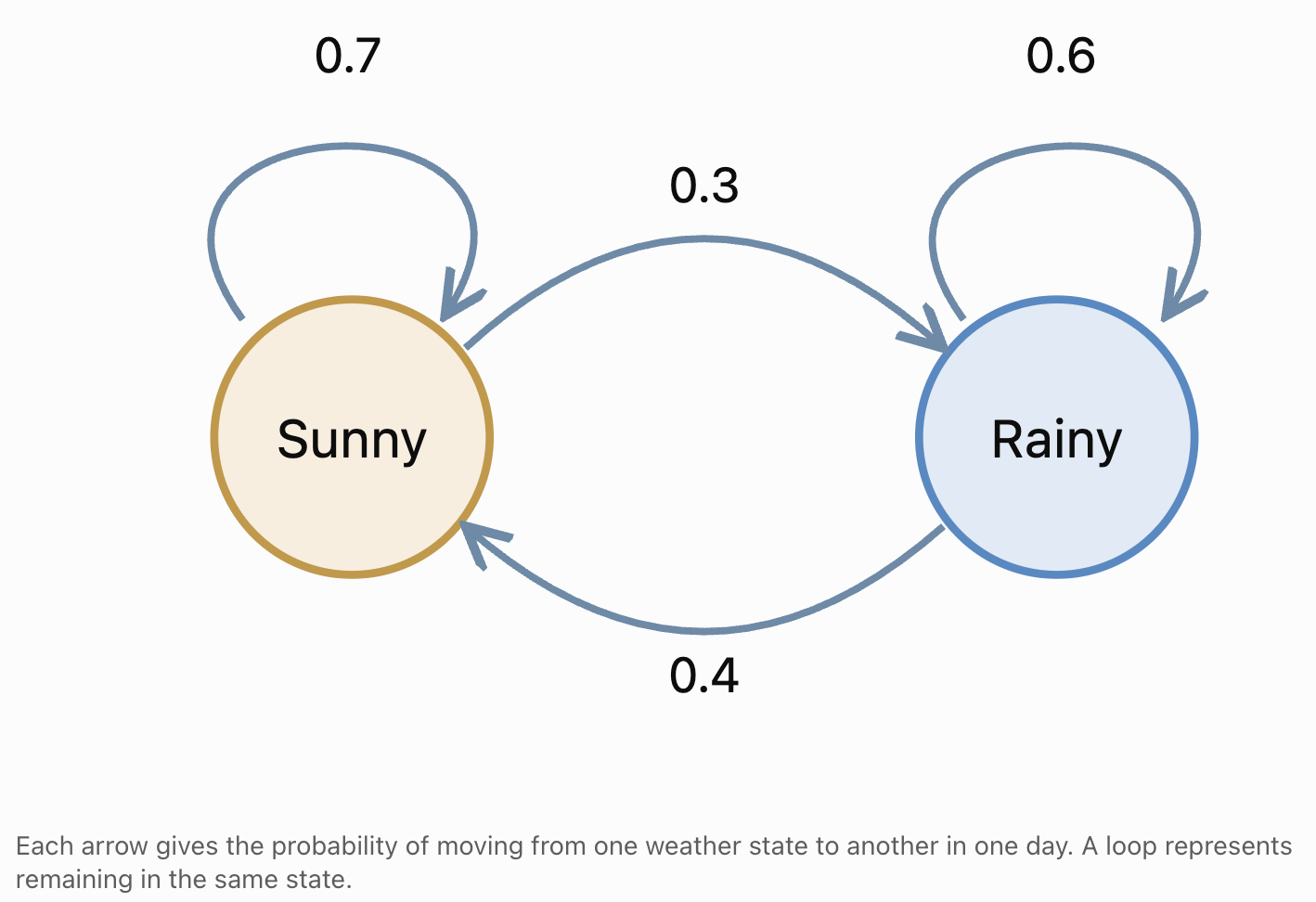
A transition diagram is a visual representation of a Markov process.

Each state is represented by a circle or node.

Arrows show possible transitions between states.

The numbers on the arrows represent transition probabilities.

Example: Sunny and Rainy Weather

Interpreting the Diagram

The arrow from Sunny to Rainy has probability 0.3.

This means:

P(Rainy tomorrow | Sunny today) = 0.3

The loop from Sunny back to Sunny has probability 0.7.

This means:

P(Sunny tomorrow | Sunny today) = 0.7

Similarly:

P(Sunny tomorrow | Rainy today) = 0.4

P(Rainy tomorrow | Rainy today) = 0.6

Transition Matrices

A transition matrix organizes transition probabilities into a rectangular array.

For the weather model, we can write:

P = [[0.7, 0.3], [0.4, 0.6]]

The rows represent the current state.

The columns represent the next state.

We will use the state order:

Sunny, Rainy

Properties of a Transition Matrix

For a finite-state Markov chain using this row convention:

• Every entry is between 0 and 1.

• Every row adds to 1.

• Each row describes the probabilities of leaving one state.

• Each column identifies the destination state.

A matrix satisfying these conditions is called a row-stochastic matrix.

Why Matrices Are Useful

Transition matrices allow us to calculate probabilities over several time steps.

They are particularly useful when a model contains many states.

Calculating One-Step Transition Probabilities

Suppose today is sunny.

Using the weather transition matrix:

P = [[0.7, 0.3], [0.4, 0.6]]

The probability that tomorrow is sunny is:

P(Sunny tomorrow | Sunny today) = 0.7

The probability that tomorrow is rainy is:

P(Rainy tomorrow | Sunny today) = 0.3

If today is rainy:

P(Sunny tomorrow | Rainy today) = 0.4

P(Rainy tomorrow | Rainy today) = 0.6

These are called one-step transition probabilities because they describe changes over one time interval.

Calculating Two-Step Transition Probabilities

Markov models can also be used to predict states several steps into the future.

Suppose today is sunny.

What is the probability that the weather will be sunny two days from now?

There are two possible paths ending in sunny weather:

• Sunny → Sunny → Sunny

• Sunny → Rainy → Sunny

Path One: Sunny, Sunny, Sunny

Probability:

0.7 × 0.7 = 0.49

Path Two: Sunny, Rainy, Sunny

Probability:

0.3 × 0.4 = 0.12

Add the Probabilities

P(Sunny in two days | Sunny today) = 0.49 + 0.12

= 0.61

There is a 61% probability that the weather will be sunny two days from now.

Why Do We Add the Paths?

The two paths are mutually exclusive.

The system cannot be both sunny and rainy on the intermediate day.

Therefore, the probabilities of the separate paths can be added.

Worked Example: Rain Two Days from Now

Suppose today is sunny.

Find the probability that it will be rainy two days from now.

Possible paths:

• Sunny → Sunny → Rainy

• Sunny → Rainy → Rainy

First path:

0.7 × 0.3 = 0.21

Second path:

0.3 × 0.6 = 0.18

Add:

P(Rainy in two days | Sunny today) = 0.21 + 0.18

= 0.39

The two-day probabilities are:

• Sunny: 0.61

• Rainy: 0.39

Check:

0.61 + 0.39 = 1

The results form a valid probability distribution.

Matrix Multiplication and Markov Processes

Transition matrices can be multiplied to calculate multi-step probabilities.

For the weather model:

P = [[0.7, 0.3], [0.4, 0.6]]

The two-step transition matrix is:

P² = P × P

Calculate each entry by multiplying corresponding row and column values and adding the results.

Sunny to Sunny

0.7 × 0.7 + 0.3 × 0.4

= 0.49 + 0.12

= 0.61

Sunny to Rainy

0.7 × 0.3 + 0.3 × 0.6

= 0.21 + 0.18

= 0.39

Rainy to Sunny

0.4 × 0.7 + 0.6 × 0.4

= 0.28 + 0.24

= 0.52

Rainy to Rainy

0.4 × 0.3 + 0.6 × 0.6

= 0.12 + 0.36

= 0.48

Therefore:

P² = [[0.61, 0.39], [0.52, 0.48]]

Notice that the rows still add to 1.

Calculating Three-Step and Longer-Term Probabilities

The same principle extends to additional time steps.

P³ = P² × P

More generally:

Pⁿ = n-step transition matrix

where n is a positive integer.

For the weather model:

P³ = [[0.583, 0.417], [0.556, 0.444]]

Therefore, if today is sunny:

P(Sunny in three days) = 0.583

P(Rainy in three days) = 0.417

The transition matrix can be raised to higher powers to calculate probabilities over many days.

This makes Markov processes useful for forecasting.

State Probability Distributions

Sometimes the current state is uncertain.

Instead of knowing that today is sunny, we might know the probabilities of the current states.

Suppose:

• Probability of sunny today = 0.6

• Probability of rainy today = 0.4

We can represent this as a state probability vector:

v₀ = [0.6, 0.4]

The entries represent the probabilities of the states in the chosen order.

Calculating Tomorrow's State Distribution

Using the row-vector convention:

v₁ = v₀P

Substitute:

v₁ = [0.6, 0.4] × [[0.7, 0.3], [0.4, 0.6]]

Sunny probability:

0.6 × 0.7 + 0.4 × 0.4

= 0.42 + 0.16

= 0.58

Rainy probability:

0.6 × 0.3 + 0.4 × 0.6

= 0.18 + 0.24

= 0.42

Therefore:

v₁ = [0.58, 0.42]

Tomorrow's predicted state probabilities are:

• Sunny: 58%

• Rainy: 42%

General Formula

For n time steps:

vₙ = v₀Pⁿ

This formula allows us to predict the probability distribution of states at future times.

Modelling a Simple Stochastic System

Consider a machine that can be in one of two states:

• Working

• Broken

Suppose:

• A working machine remains working the next day with probability 0.9.

• A working machine becomes broken with probability 0.1.

• A broken machine is repaired and working the next day with probability 0.6.

• A broken machine remains broken with probability 0.4.

Transition Matrix

Using the state order Working, Broken:

P = [[0.9, 0.1], [0.6, 0.4]]

One-Step Interpretation

If the machine is working today:

P(Working tomorrow) = 0.9

P(Broken tomorrow) = 0.1

If the machine is broken today:

P(Working tomorrow) = 0.6

P(Broken tomorrow) = 0.4

Two-Step Probability of Remaining Operational

Suppose the machine is working today.

What is the probability that it is working two days from now?

There are two possible paths:

Working → Working → Working

Working → Broken → Working

Calculate:

P(Working after two days) = 0.9 × 0.9 + 0.1 × 0.6

= 0.81 + 0.06

= 0.87

There is an 87% probability that the machine will be working two days from now.

Absorbing States

An absorbing state is a state that cannot be left once the system enters it.

The probability of remaining in an absorbing state is 1.

Example: Equipment Failure Without Repair

Suppose a machine can be:

• Working

• Permanently failed

Once the machine permanently fails, it cannot return to the working state.

The transition matrix might be:

P = [[0.95, 0.05], [0, 1]]

The failed state is absorbing because:

P(Failed next | Failed now) = 1

Applications of Absorbing States

Absorbing states are useful for modelling:

• Permanent equipment failure.

• Completion of a task.

• Graduation from a programme.

• Reaching a final stage in a game.

• Extinction of a population in a simplified ecological model.

Steady-State Probabilities

Some Markov chains approach a stable probability distribution over time.

This is called a steady-state distribution or stationary distribution.

A stationary distribution remains unchanged after one transition.

If π is a stationary distribution, then:

πP = π

The entries of π must also add to 1.

Worked Example: Long-Term Weather Probabilities

Recall the weather transition matrix:

P = [[0.7, 0.3], [0.4, 0.6]]

Let:

s = long-term probability of sunny weather

r = long-term probability of rainy weather

We know:

s + r = 1

At steady state:

s = 0.7s + 0.4r

Rearrange:

0.3s = 0.4r

Therefore:

3s = 4r

So:

s = (4/3)r

Substitute into:

s + r = 1

(4/3)r + r = 1

(7/3)r = 1

r = 3/7

Therefore:

s = 4/7

Final Answer

Sunny ≈ 57.14%

Rainy ≈ 42.86%

In this model, the long-term state distribution approaches approximately 57.14% sunny and 42.86% rainy.

Important Distinction

A steady-state distribution does not mean the weather stops changing.

The system continues moving between sunny and rainy states.

The long-term probabilities become stable even though individual outcomes remain uncertain.

Not every Markov chain converges to a unique stationary distribution from every starting state.

Practical Application: Customer Brand Loyalty

Businesses can use Markov models to study customer behaviour.

Suppose customers choose between two brands:

• Brand A

• Brand B

Each month:

• 80% of Brand A customers remain with Brand A.

• 20% switch to Brand B.

• 30% of Brand B customers switch to Brand A.

• 70% remain with Brand B.

Transition Matrix

P = [[0.8, 0.2], [0.3, 0.7]]

Suppose the initial market shares are:

Brand A = 60%

Brand B = 40%

The initial state vector is:

v₀ = [0.6, 0.4]

Calculate Next Month's Market Shares

v₁ = v₀P

Brand A:

0.6 × 0.8 + 0.4 × 0.3

= 0.48 + 0.12

= 0.60

Brand B:

0.6 × 0.2 + 0.4 × 0.7

= 0.12 + 0.28

= 0.40

Therefore:

v₁ = [0.6, 0.4]

The market shares remain unchanged.

This initial distribution is already a stationary distribution for the model.

Interpretation

Even though some customers switch brands each month, the overall market shares can remain constant.

This demonstrates how a system can experience individual changes while maintaining stable overall proportions.

Practical Application: Animal Movement

Ecologists can use Markov processes to model animal movement between habitats.

Suppose a population of animals moves between:

• Forest

• Grassland

Each day:

• 85% of animals in the forest remain there.

• 15% move to grassland.

• 25% of animals in grassland move to forest.

• 75% remain in grassland.

The transition matrix is:

P = [[0.85, 0.15], [0.25, 0.75]]

Suppose initially:

• 70% of animals are in the forest.

• 30% are in grassland.

Then:

v₀ = [0.7, 0.3]

Predict the Next Day

Forest:

0.7 × 0.85 + 0.3 × 0.25

= 0.595 + 0.075

= 0.67

Grassland:

0.7 × 0.15 + 0.3 × 0.75

= 0.105 + 0.225

= 0.33

Therefore:

v₁ = [0.67, 0.33]

The model predicts:

• 67% in forest.

• 33% in grassland.

Real-World Limitations

Actual animal movement may depend on:

• Food availability.

• Weather.

• Predators.

• Seasonal changes.

• Habitat destruction.

• Reproductive behaviour.

A simple Markov model may need additional states or changing transition probabilities to represent these factors accurately.

Practical Application: Student Learning Progress

Markov models can also describe movement between learning stages.

Suppose students are classified into three states:

• Beginning

• Developing

• Proficient

A simplified transition matrix might be:

Each row adds to 1.

For example, a student currently at the Developing level has:

• 10% probability of moving to Beginning.

• 60% probability of remaining Developing.

• 30% probability of moving to Proficient.

Interpretation

A school could use such a model to estimate future distributions of achievement levels.

However, learning is influenced by teaching quality, motivation, prior knowledge, attendance, and other factors.

A simple Markov model should not be interpreted as a fixed prediction of an individual student's future achievement.

Time-Homogeneous and Time-Varying Markov Chains

Many introductory Markov models assume that transition probabilities remain constant over time.

These are called time-homogeneous Markov chains.

For example:

P(Sunny tomorrow | Sunny today) = 0.7

remains the same throughout the model.

However, some real systems change over time.

Time-Varying Example

A machine may become more likely to fail as it ages.

Its transition probabilities may therefore change each month.

Similarly, animal movement probabilities may change with the seasons.

Such systems can be modelled using different transition matrices at different time steps.

Important Distinction

The Markov property does not require transition probabilities to remain constant over time.

It requires that the next-state probabilities depend on the current state rather than the complete past history.

Evaluating Markov Models

Markov models simplify complex systems.

Their usefulness depends on whether the assumptions reasonably describe the situation.

Questions to Consider

Are the states clearly defined?

Every possible situation should correspond to an appropriate state.

Does the current state contain enough information?

If earlier history influences the future beyond what is represented by the current state, the simple Markov assumption may be unsuitable.

Are the transition probabilities realistic?

Probabilities should be estimated using suitable observations or justified assumptions.

Do the probabilities add to 1?

Every row of the transition matrix must add to 1.

Are transition probabilities constant?

If not, a time-varying model may be needed.

Does the model accurately represent the system?

Predictions should be compared with real observations when possible.

A Strategy for Solving Markov Problems

When solving a Markov process problem, use the following steps.

Identify the states.

Determine the possible conditions of the system.

Choose a consistent state order.

For example:

Sunny, Rainy

Identify the transition probabilities.

Determine the probability of moving from each current state to every possible next state.

Construct the transition matrix.

Place the current states in rows and next states in columns.

Check the matrix.

Ensure all entries are between 0 and 1 and each row adds to 1.

Determine the initial state.

The initial state may be known exactly or represented by a probability distribution.

Calculate the required probabilities.

Use probability paths, matrix multiplication, or state vectors.

Interpret the results.

Explain what the calculated probabilities mean in the context of the problem.

Evaluate the model.

Consider whether the assumptions are realistic.

Common Mistakes

Confusing a Markov process with a deterministic process

A Markov process describes probabilistic transitions rather than guaranteed outcomes.

Assuming the future is independent of the present

The Markov property means that the future depends on the current state, not that all states are independent.

Confusing the Markov property with complete randomness

Markov processes can contain strong relationships between consecutive states.

Reading a transition matrix incorrectly

Always identify whether rows or columns represent the current state.

Forgetting that transition probabilities must add to 1

Every row must represent a complete probability distribution of possible next states.

Multiplying transition probabilities incorrectly

For multi-step transitions, consider every possible intermediate state.

Forgetting to add alternative paths

Different paths may lead to the same final state.

Confusing one-step and two-step probabilities

P gives one-step transitions, while P² gives two-step transitions.

Assuming a steady state means no changes occur

A stationary distribution can remain constant even while individual states continue changing.

Assuming every Markov chain reaches the same steady state

Some chains do not converge to a unique stationary distribution.

Ignoring real-world limitations

Actual systems may require more states, additional variables, or changing transition probabilities.

Key Terms

• Markov Process: A stochastic process in which the next-state probabilities depend on the current state rather than the complete history.

• Markov Chain: A Markov process with a discrete set of states and discrete time steps.

• Stochastic Process: A mathematical model describing a system that changes over time with an element of randomness.

• Deterministic Process: A process whose future states are fully determined by its current conditions and rules.

• State: A possible condition of a system at a particular time.

• State Space: The set of all possible states in a model.

• Markov Property: The property that the current state contains all information from the past needed to predict the next state.

• Transition: A movement from one state to another.

• Transition Probability: The probability of moving from one state to another during a specified time step.

• Transition Diagram: A diagram showing states as nodes and transitions as arrows.

• Transition Matrix: A matrix containing the probabilities of moving between states.

• Stochastic Matrix: A matrix containing non-negative probabilities whose rows or columns sum to 1, depending on the convention.

• Row-Stochastic Matrix: A transition matrix in which every row sums to 1.

• One-Step Probability: The probability of moving between states in one time interval.

• Multi-Step Probability: The probability of moving between states over several time intervals.

• State Vector: A vector describing the probabilities of the possible states at a particular time.

• Initial Distribution: The probability distribution of states at the beginning of a process.

• Matrix Multiplication: A mathematical operation used to combine transition probabilities.

• Absorbing State: A state that cannot be left once entered.

• Stationary Distribution: A probability distribution that remains unchanged after applying the transition matrix.

• Steady State: A stable probability distribution that may describe the long-term behaviour of a Markov chain.

• Time-Homogeneous Markov Chain: A Markov chain whose transition probabilities remain constant over time.

• Time-Varying Markov Chain: A Markov chain whose transition probabilities can change over time.

• Probability Model: A mathematical representation of uncertain outcomes.

• Stochastic Modelling: The use of mathematical models to describe systems involving randomness.

Key Takeaways

• Markov processes describe systems that move between states according to probabilities.

• The Markov property states that the next state depends on the current state rather than the complete history.

• Markov chains are commonly used to model systems with discrete states and discrete time steps.

• Transition probabilities describe the likelihood of moving from one state to another.

• Transition diagrams use nodes and arrows to represent states and transitions.

• Transition matrices organize transition probabilities into rows and columns.

• In a row-stochastic transition matrix, every row must add to 1.

• One-step transition probabilities describe changes over one time interval.

• Two-step probabilities can be calculated by considering all possible intermediate states.

• Matrix multiplication provides an efficient way to calculate multi-step probabilities.

• P² represents two-step transition probabilities, while Pⁿ represents n-step probabilities.

• State vectors describe the probability distribution of the system across its possible states.

• The formula vₙ = v₀Pⁿ predicts state distributions after n time steps using the row-vector convention.

• Absorbing states cannot be left once entered.

• Some Markov chains approach stable long-term probability distributions.

• A stationary distribution satisfies πP = π.

• A steady-state distribution does not mean that individual state changes stop.

• Markov models are useful in weather forecasting, manufacturing, ecology, customer behaviour, education, and engineering.

• The accuracy of a Markov model depends on its assumptions, state definitions, and transition probabilities.

Check Your Understanding

Recall and Understanding

1. Define a Markov process and explain the Markov property.

2. Explain the difference between a deterministic process and a stochastic process.

3. Define a state and a transition probability.

4. Explain how a transition diagram represents a Markov chain.

5. State the requirements for a valid row-stochastic transition matrix.

Application

6. A weather model has two states, Sunny and Rainy. If P(Sunny → Sunny) = 0.8 and P(Rainy → Sunny) = 0.3, construct the transition matrix.

7. A machine has a 90% probability of remaining operational and a 10% probability of failing each day when working. A failed machine has a 60% probability of being repaired by the next day. Construct a transition matrix.

8. Using the weather matrix P = [[0.7, 0.3], [0.4, 0.6]], calculate the probability that it is sunny two days from now if today is rainy.

9. A Markov chain has transition matrix P = [[0.6, 0.4], [0.2, 0.8]]. Calculate P².

10. A system has initial state vector v₀ = [0.3, 0.7] and transition matrix P = [[0.8, 0.2], [0.5, 0.5]]. Calculate the state distribution after one step.

Analysis and Challenge

11. A customer loyalty model has transition matrix P = [[0.85, 0.15], [0.25, 0.75]]. If 60% of customers initially use Brand A, calculate the expected market shares after two months.

12. Explain why the Markov property does not mean that consecutive states are independent.

13. A machine has states Working and Permanently Failed, with transition matrix P = [[0.95, 0.05], [0, 1]]. Identify the absorbing state and calculate the probability that a machine working initially has permanently failed after two time steps.

14. Find the stationary distribution for the transition matrix P = [[0.8, 0.2], [0.3, 0.7]].

15. Design a simple three-state Markov model for student learning progress, animal movement, or weather conditions. Construct a valid transition matrix, explain your probabilities, and describe one limitation of your model.

Final Summary

Markov processes provide a mathematical framework for describing systems that change between states according to probabilities.

The defining feature of a Markov process is that the next-state probabilities depend on the current state rather than the complete history of previous states.

Transition diagrams and transition matrices allow these probabilities to be represented clearly.

By multiplying transition matrices and using state probability vectors, we can calculate the likelihood of future states and investigate long-term behaviour.

Markov models are valuable tools for analysing weather patterns, equipment reliability, customer behaviour, animal movement, and other systems involving uncertainty.

Understanding their assumptions and limitations is essential for constructing useful models and interpreting their predictions accurately.