Continuous Probability Distributions

Introduction to Continuous Probability Distributions

Many situations involve measurements that can take any value within a range.

For example:

• The height of a student.

• The time required to complete a race.

• The mass of a manufactured product.

• The temperature of a liquid.

• The lifetime of a battery.

• The amount of rainfall during a storm.

Unlike counting the number of customers or rolling a die, these situations involve quantities that can vary continuously.

A continuous probability distribution describes how probability is distributed across the possible values of a continuous random variable.

Instead of assigning probabilities to individual values, continuous distributions assign probabilities to intervals of values.

Understanding continuous probability distributions allows us to calculate the likelihood of measurements falling within particular ranges, compare different probability models, and make predictions about real-world situations.

Reviewing Random Variables

A random variable is a variable that assigns a numerical value to the outcome of a random experiment.

Random variables are generally classified as either discrete or continuous.

Discrete Random Variables

A discrete random variable takes values from a finite or countably infinite set.

Examples include:

• Number of students absent.

• Number of defective products.

• Number of goals scored.

• Number of heads in five coin tosses.

Discrete random variables usually arise from counting.

Continuous Random Variables

A continuous random variable can take any real value within an interval or collection of intervals.

Examples include:

• Height.

• Mass.

• Time.

• Distance.

• Temperature.

Continuous random variables usually arise from measurement.

Comparing Discrete and Continuous Variables

An important distinction is that continuous measurements are not limited to the number of decimal places shown by an instrument.

For example, a stopwatch may display 12.45 seconds, but the actual elapsed time can have greater precision.

Understanding Continuous Probability Models

A continuous probability model describes how likely different ranges of values are.

Suppose X represents the time required for a student to travel to school.

Possible values might include:

12.4 minutes

12.43 minutes

12.437 minutes

12.4372 minutes

Because infinitely many values are possible within an interval, it is not useful to assign a separate positive probability to every exact value.

Instead, probabilities are calculated over intervals.

For example:

• P(10 ≤ X ≤ 15)

• P(X > 20)

• P(12 < X < 18)

These expressions describe the probability that the random variable falls within a particular range.

Probability Density Functions

A probability density function, or PDF, describes how probability is distributed across the values of a continuous random variable.

It is usually written as:

f(x)

The function f(x) represents probability density, not the probability of one exact value.

Two Essential Properties

A valid probability density function must satisfy two conditions.

The density cannot be negative.

f(x) ≥ 0

The total area under the density curve must equal 1.

Total area = 1

This represents 100% of all possible outcomes.

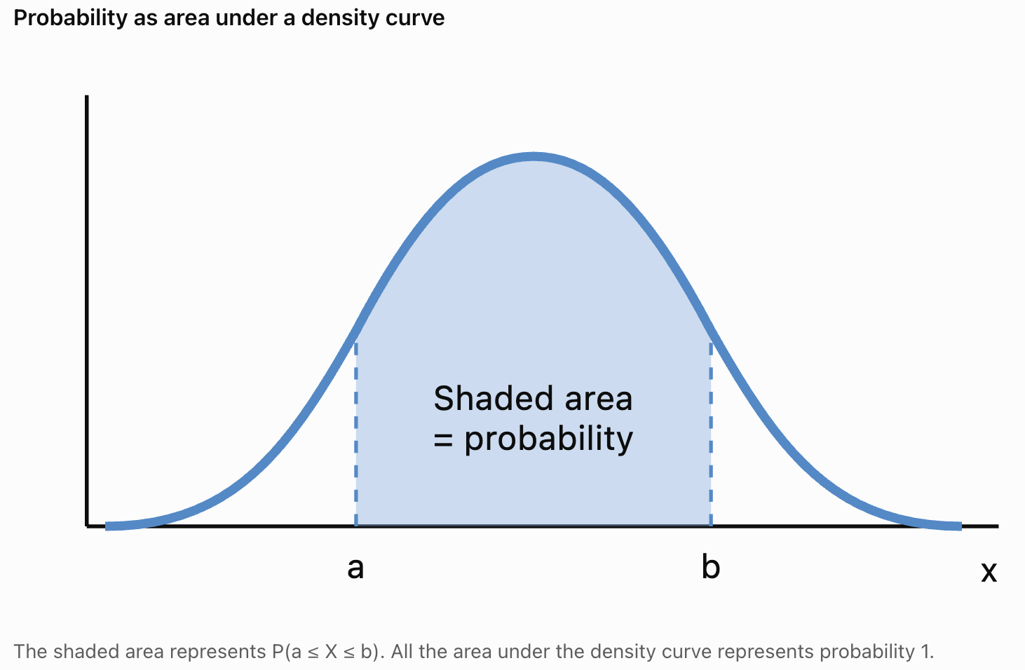
Understanding Density

A higher density indicates that probability is more concentrated near that region.

A lower density indicates that probability is less concentrated.

However, the height of the curve is not itself a probability.

Probability is represented by area under the curve.

Why Exact Values Have Zero Probability

For a continuous random variable:

P(X = a) = 0

for any individual value a.

This may seem surprising.

For example, suppose X represents the height of a randomly selected student.

The probability that the student's height is exactly 170.000000... cm is zero in a continuous model.

However, the probability that the height lies between 169 cm and 171 cm can be positive.

Why?

Probability is represented by area.

A single exact value has no width, so the area associated with that value is zero.

This does not mean the value is impossible.

It means that probability must be considered over intervals.

Important Consequence

For continuous random variables:

P(a ≤ X ≤ b) = P(a < X < b)

Including or excluding the endpoints does not change the probability.

This is different from discrete probability distributions, where endpoints may contain positive probability.

Calculating Probabilities Using Area

The probability that a continuous random variable lies between a and b is the area under the density curve between those values.

In calculus notation:

P(a ≤ X ≤ b) = ∫ₐᵇ f(x) dx

The integral symbol represents the accumulation of area under the curve.

Students who have not yet studied integration can calculate probabilities using geometric areas when the density graph has a simple shape.

Common shapes include:

• Rectangles.

• Triangles.

• Trapezoids.

The Continuous Uniform Distribution

A continuous uniform distribution describes a random variable whose probability density is constant across a specified interval.

This means equal-length intervals within the range have equal probabilities.

For example, suppose a bus arrives at a randomly selected time between 0 and 10 minutes.

If every arrival time in that interval is equally likely in the continuous sense, the waiting time can be modelled using a uniform distribution.

Uniform Distribution Notation

X ~ U(a, b)

where:

• a is the minimum possible value.

• b is the maximum possible value.

The probability density function is:

f(x) = 1/(b − a) for a ≤ x ≤ b

and:

f(x) = 0 outside this interval.

Why Does This Formula Work?

The density graph forms a rectangle.

Its width is:

b − a

Its height is:

1/(b − a)

Therefore:

Area = width × height

= (b − a) × 1/(b − a)

= 1

The total probability is exactly 1.

Worked Example: Uniform Waiting Times

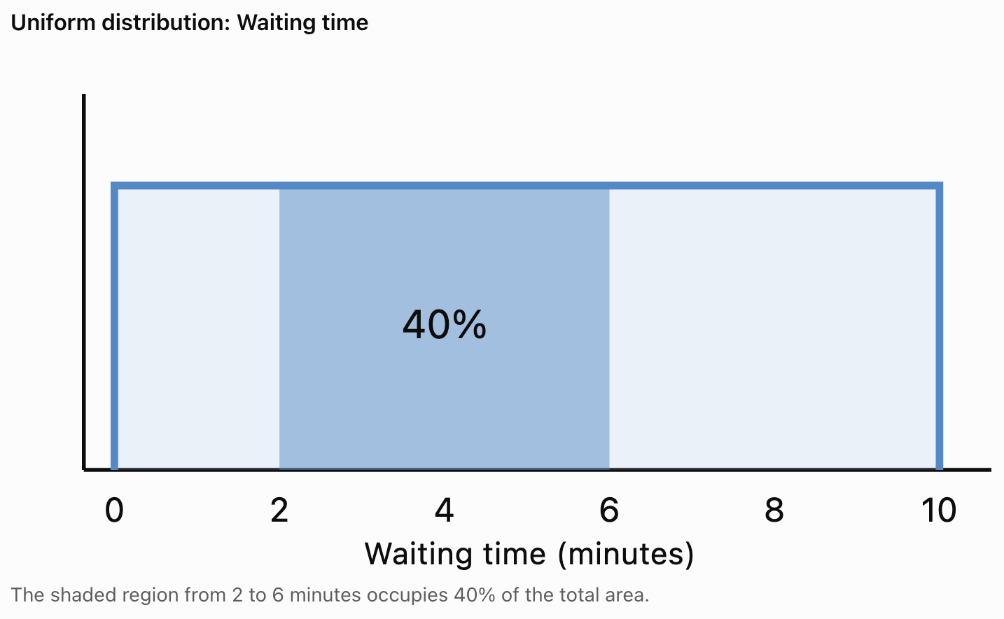
A bus arrives at a uniformly random time between 0 and 10 minutes after a passenger begins waiting.

Let X represent the waiting time.

X ~ U(0, 10)

Find the probability that the passenger waits between 2 and 6 minutes.

Step 1: Determine the Total Interval

Total interval length:

10 − 0 = 10 minutes

Step 2: Determine the Favourable Interval

Favourable interval length:

6 − 2 = 4 minutes

Step 3: Calculate the Probability

For a uniform distribution:

Probability = Favourable interval length / Total interval length

P(2 ≤ X ≤ 6) = 4/10

P(2 ≤ X ≤ 6) = 0.40

There is a 40% probability that the waiting time is between two and six minutes.

More Uniform Distribution Problems

Worked Example: Waiting Less Than Three Minutes

Suppose:

X ~ U(0, 12)

Find:

P(X < 3)

The favourable interval is from 0 to 3.

Its length is:

3 − 0 = 3

The total interval length is:

12 − 0 = 12

Therefore:

P(X < 3) = 3/12

P(X < 3) = 0.25

There is a 25% probability of waiting less than three minutes.

Worked Example: Waiting More Than Eight Minutes

Using the same distribution:

X ~ U(0, 12)

Find:

P(X > 8)

The favourable interval is from 8 to 12.

Its length is:

12 − 8 = 4

Therefore:

P(X > 8) = 4/12

P(X > 8) = 1/3 ≈ 0.3333

There is approximately a 33.33% probability of waiting more than eight minutes.

Expected Value and Variance of a Uniform Distribution

For a continuous uniform distribution:

X ~ U(a, b)

The expected value is:

E(X) = (a + b)/2

The variance is:

Var(X) = (b − a)²/12

The standard deviation is:

σ = (b − a)/√12

Worked Example

Suppose:

X ~ U(4, 16)

Expected value:

E(X) = (4 + 16)/2

E(X) = 10

Variance:

Var(X) = (16 − 4)²/12

= 144/12

Var(X) = 12

Standard deviation:

σ = √12

σ ≈ 3.46

The distribution has a mean of 10 and a standard deviation of approximately 3.46.

Non-Uniform Continuous Distributions

Not all continuous distributions have constant density.

Some values may be more common than others.

For example:

• Adult heights may cluster around a central value.

• Manufacturing measurements may concentrate near a target.

• Waiting times may be more common near shorter durations.

• Certain natural measurements may have asymmetrical distributions.

These situations require different probability density functions.

A density curve may be:

• Symmetrical.

• Skewed to the left.

• Skewed to the right.

• Uniform.

• Bell-shaped.

The Normal Distribution

One of the most important continuous probability distributions is the normal distribution.

A normal distribution has a symmetrical, bell-shaped curve.

Its shape is determined by two parameters:

• Mean, μ.

• Standard deviation, σ.

The mean determines the centre of the distribution.

The standard deviation determines how spread out the values are.

Properties of the Normal Distribution

• The curve is symmetrical around the mean.

• The mean, median, and mode are equal.

• The total area under the curve equals 1.

• The curve approaches the horizontal axis without touching it.

• Values near the mean are more common than values far from the mean.

Examples of Approximately Normal Data

Some measurements may be approximately normally distributed, including:

• Heights within certain populations.

• Certain measurement errors.

• Some manufacturing dimensions.

• Some standardized assessment scores.

However, not every real-world dataset follows a normal distribution.

The Empirical Rule

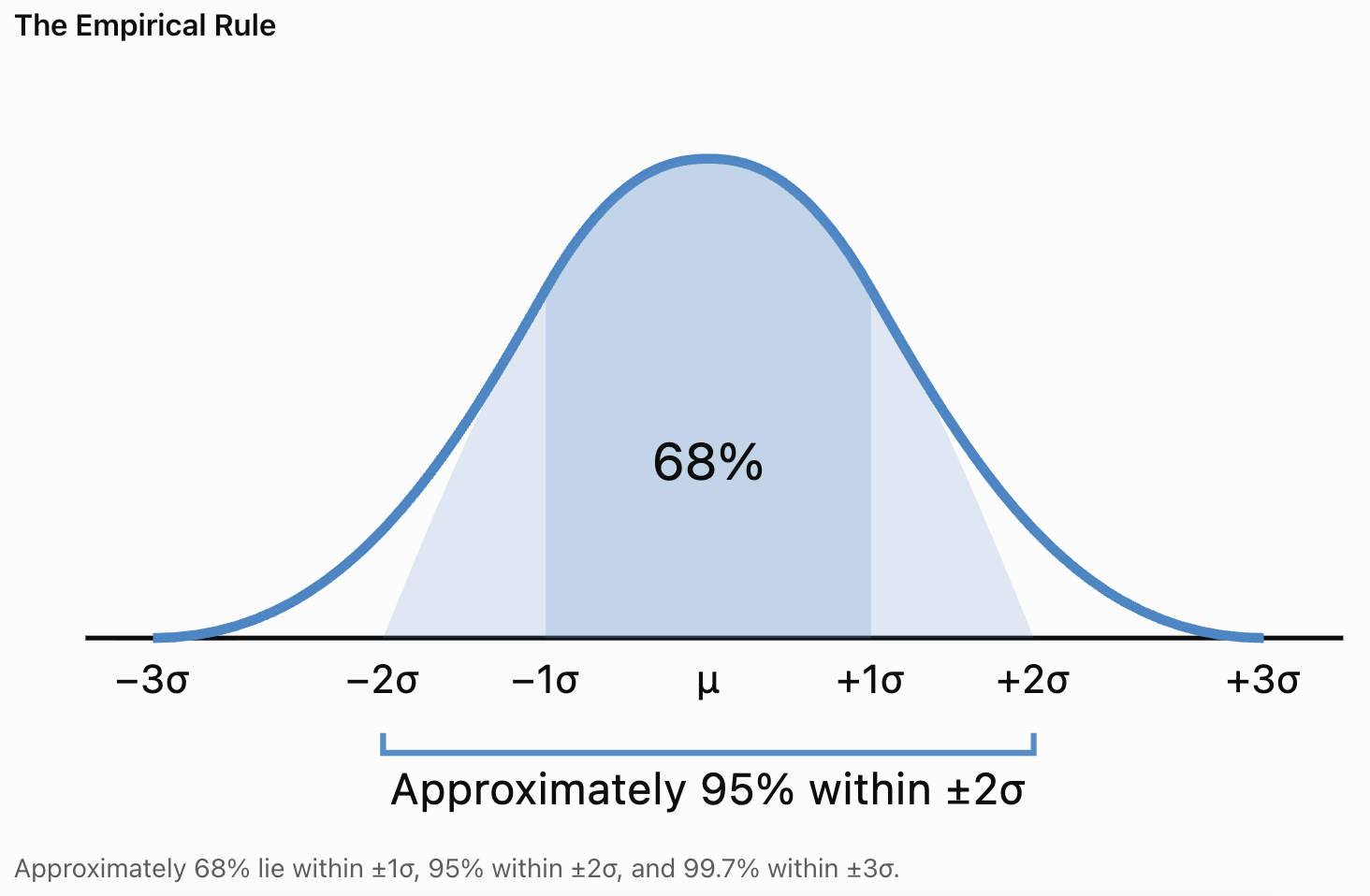
For a normal distribution:

• Approximately 68% of values lie within one standard deviation of the mean.

• Approximately 95% lie within two standard deviations.

• Approximately 99.7% lie within three standard deviations.

This is known as the Empirical Rule.

Worked Example: Normally Distributed Test Scores

Suppose examination scores are approximately normally distributed with:

Mean = 70

Standard deviation = 10

Within One Standard Deviation

Lower boundary:

70 − 10 = 60

Upper boundary:

70 + 10 = 80

Approximately 68% of students score between 60 and 80.

Within Two Standard Deviations

Lower boundary:

70 − 20 = 50

Upper boundary:

70 + 20 = 90

Approximately 95% of students score between 50 and 90.

Within Three Standard Deviations

Lower boundary:

70 − 30 = 40

Upper boundary:

70 + 30 = 100

Approximately 99.7% of students score between 40 and 100.

These are approximate results based on the normal model.

Standardizing Normal Distributions

Normal distributions can have different means and standard deviations.

To compare values from different normal distributions, we use a z-score.

The formula is:

z = (x − μ)/σ

where:

• x is the observed value.

• μ is the mean.

• σ is the standard deviation.

A z-score describes how many standard deviations a value lies above or below the mean.

Interpreting z-Scores

• z = 0 means the value equals the mean.

• z = 1 means the value is one standard deviation above the mean.

• z = −1 means the value is one standard deviation below the mean.

• z = 2 means the value is two standard deviations above the mean.

Worked Example

A student scores 85 on a test.

The mean is 70, and the standard deviation is 10.

Calculate the z-score.

z = (85 − 70)/10

= 15/10

z = 1.5

The student's score is 1.5 standard deviations above the mean.

Calculating Normal Probabilities

Normal probabilities are calculated using areas under the normal curve.

Because the normal curve is not a simple geometric shape, exact probabilities usually require integration or numerical methods.

In practice, students often use:

• Standard normal distribution tables.

• Scientific calculators.

• Spreadsheet software.

• Statistical software.

Worked Example: Probability Below a Value

Suppose:

X is normally distributed with mean 100 and standard deviation 15.

Find the probability that X is less than 115.

Step 1: Calculate the z-Score

z = (115 − 100)/15

z = 1

Step 2: Use a Standard Normal Table

For z = 1:

P(Z < 1) ≈ 0.8413

Final answer:

P(X < 115) ≈ 0.8413

There is approximately an 84.13% probability that X is below 115.

Worked Example: Probability Above a Value

Using the same distribution, find:

P(X > 115)

Use complementary probability:

P(X > 115) = 1 − P(X ≤ 115)

= 1 − 0.8413

P(X > 115) ≈ 0.1587

There is approximately a 15.87% probability that X exceeds 115.

Calculating Probabilities Between Two Values

Suppose:

X is normally distributed with:

μ = 100

σ = 15

Find:

P(85 < X < 115)

Step 1: Calculate the Lower z-Score

z₁ = (85 − 100)/15

z₁ = −1

Step 2: Calculate the Upper z-Score

z₂ = (115 − 100)/15

z₂ = 1

Step 3: Use Standard Normal Probabilities

P(Z < 1) ≈ 0.8413

P(Z < −1) ≈ 0.1587

Subtract:

P(−1 < Z < 1) = 0.8413 − 0.1587

P(85 < X < 115) ≈ 0.6826

Approximately 68.26% of values lie within one standard deviation of the mean.

This agrees with the Empirical Rule.

Other Continuous Probability Models

Different continuous distributions describe different types of uncertainty.

Exponential Distribution

The exponential distribution is often used to model waiting times between events in a Poisson process.

Examples include:

• Time between customer arrivals.

• Time between telephone calls.

• Waiting time until the next randomly occurring event.

For an exponential distribution with rate λ:

f(x) = λe^(−λx) for x ≥ 0

The expected waiting time is:

E(X) = 1/λ

If events occur at an average rate of four per hour, the expected waiting time between events is:

1/4 hour = 15 minutes

Triangular Distribution

A triangular distribution is sometimes used when a minimum, maximum, and most likely value can be estimated.

It can be useful for simplified modelling of project durations or uncertain measurements.

Uniform Distribution

A uniform distribution is appropriate when equal-length intervals within a range are equally likely.

Normal Distribution

A normal distribution is appropriate for certain measurements that cluster symmetrically around a mean.

The correct model depends on the characteristics of the data and the assumptions being made.

Comparing Discrete and Continuous Probability Models

Discrete and continuous distributions both describe uncertainty, but they assign probabilities differently.

Discrete Example: Rolling a Die

A fair die has six possible outcomes.

The probability of rolling exactly three is:

P(X = 3) = 1/6

This is a positive probability assigned to a single value.

Continuous Example: Measuring Height

Suppose X represents a student's height.

The probability of an exact height is:

P(X = 170 cm) = 0

However:

P(169 ≤ X ≤ 171)

may be positive.

Probability Mass Versus Probability Density

For a discrete distribution, individual outcomes can have probability mass.

For a continuous distribution, probabilities are obtained by accumulating density over intervals.

This is why discrete distributions are commonly displayed with separate bars, while continuous distributions are displayed using density curves.

Practical Application: Manufacturing

A factory manufactures metal rods with a target length of 50 cm.

Suppose rod lengths are approximately normally distributed with:

Mean = 50 cm

Standard deviation = 0.2 cm

The factory accepts rods with lengths between 49.6 cm and 50.4 cm.

Step 1: Calculate z-Scores

Lower boundary:

z₁ = (49.6 − 50)/0.2

z₁ = −2

Upper boundary:

z₂ = (50.4 − 50)/0.2

z₂ = 2

Step 2: Interpret the Interval

The accepted lengths are within two standard deviations of the mean.

Using the Empirical Rule:

Approximately 95% of rods fall within this range.

Using standard normal probabilities gives a more precise result of approximately 95.45%.

Interpretation

The company can estimate that approximately 95.45% of rods will meet the length requirement if the normal model is accurate.

Practical Application: Travel Times

Suppose a student's travel time to school is approximately normally distributed with:

Mean = 25 minutes

Standard deviation = 5 minutes

What is the probability that the journey takes longer than 30 minutes?

Step 1: Calculate the z-Score

z = (30 − 25)/5

z = 1

Step 2: Find the Probability

P(Z > 1) ≈ 0.1587

Final answer:

There is approximately a 15.87% probability that the journey takes longer than 30 minutes.

Practical Interpretation

This information can help the student decide how much extra travel time to allow.

However, actual travel times may not follow a normal distribution, particularly when traffic delays create a long right-hand tail.

The model should be checked against observed data.

Practical Application: Battery Lifetimes

Suppose battery lifetimes are approximately normally distributed with:

Mean = 100 hours

Standard deviation = 10 hours

Find the probability that a battery lasts less than 80 hours.

Step 1: Calculate the z-Score

z = (80 − 100)/10

z = −2

Step 2: Find the Probability

P(Z < −2) ≈ 0.0228

Final answer:

There is approximately a 2.28% probability that a battery lasts less than 80 hours.

This type of analysis can help manufacturers estimate reliability and warranty risks.

Selecting an Appropriate Continuous Probability Model

When choosing a continuous probability model, consider the nature of the variable.

Uniform Model

Use when values are equally likely across equal-length intervals within a fixed range.

Example:

A random arrival time uniformly distributed between 0 and 10 minutes.

Normal Model

Use when measurements are approximately symmetrical and cluster around a mean.

Example:

Certain manufacturing dimensions or measurement errors.

Exponential Model

Use when modelling waiting times between events in a constant-rate Poisson process.

Example:

Time until the next customer arrives, assuming Poisson arrivals.

Questions to Ask

• Is the variable measured rather than counted?

• What values are possible?

• Is the distribution symmetrical or skewed?

• Are there natural minimum or maximum values?

• Does the model fit the observed data?

• Are the model assumptions reasonable?

Selecting an appropriate distribution is an important part of mathematical modelling.

Common Mistakes

Confusing probability density with probability

The height of a density curve is not the probability of an exact outcome.

Assuming exact values have positive probability

For continuous random variables, the probability of any single exact value is zero.

Forgetting that total area equals 1

A valid probability density function must have total area 1.

Using the wrong interval length

Uniform probabilities depend on the length of the favourable interval relative to the total interval.

Confusing discrete and continuous variables

Counting usually produces discrete variables, while measurement often produces continuous variables.

Using normal-distribution rules for every dataset

Not all continuous data follow a normal distribution.

Forgetting to standardize values

Normal probability calculations often require converting values into z-scores.

Using variance instead of standard deviation

The z-score formula uses standard deviation, not variance.

Forgetting complementary probability

Probabilities above a threshold can often be calculated using 1 minus the probability below that threshold.

Ignoring model assumptions

Real-world measurements may not follow the assumed distribution.

Key Terms

• Continuous Random Variable: A random variable that can take any real value within an interval or collection of intervals.

• Discrete Random Variable: A random variable with a finite or countably infinite set of possible values.

• Continuous Probability Distribution: A probability model describing how probability is distributed across continuous values.

• Probability Density Function: A non-negative function whose area over an interval gives the probability of values falling in that interval.

• Probability Density: The concentration of probability around a region of values.

• Probability Mass Function: A function assigning probabilities to individual values of a discrete random variable.

• Interval: A range of values between specified boundaries.

• Uniform Distribution: A distribution with constant probability density across a specified interval.

• Normal Distribution: A symmetrical, bell-shaped continuous probability distribution.

• Exponential Distribution: A continuous distribution often used to model waiting times between events in a Poisson process.

• Triangular Distribution: A continuous distribution with a triangular density shape.

• Mean: The average or central value of a distribution.

• Expected Value: The long-run average value of a random variable.

• Variance: A measure of the average squared deviation from the mean.

• Standard Deviation: The positive square root of variance.

• Z-Score: The number of standard deviations a value lies above or below the mean.

• Standard Normal Distribution: A normal distribution with mean 0 and standard deviation 1.

• Empirical Rule: The approximate 68–95–99.7 pattern for normal distributions.

• Cumulative Probability: The probability that a random variable is less than or equal to a specified value.

• Complementary Probability: The probability that an event does not occur.

• Area Under the Curve: The geometric representation of probability in a continuous distribution.

• Probability Model: A mathematical representation of uncertain outcomes.

• Mathematical Modelling: The process of representing real-world situations using mathematical relationships and assumptions.

Key Takeaways

• Continuous probability distributions describe random variables that can take values across continuous intervals.

• Continuous random variables often represent measurements such as time, height, mass, and temperature.

• Probabilities for continuous variables are calculated over intervals rather than at individual exact values.

• A probability density function describes how probability is distributed across possible values.

• The total area under a probability density curve equals 1.

• The probability of any exact value in a continuous distribution is zero.

• Probability over an interval is represented by the area under the density curve across that interval.

• Uniform distributions have constant density across a specified range.

• For a uniform distribution, probabilities can be calculated using interval lengths.

• Normal distributions are symmetrical and bell-shaped.

• The mean determines the centre of a normal distribution, while standard deviation determines its spread.

• The Empirical Rule describes approximate probabilities within one, two, and three standard deviations of the mean.

• Z-scores allow values from different normal distributions to be compared.

• Exponential distributions are useful for modelling certain waiting times.

• Discrete distributions assign probability mass to individual values, while continuous distributions assign probability through density over intervals.

• Continuous probability models are useful in manufacturing, transportation, science, engineering, and reliability analysis.

• Choosing an appropriate probability model requires understanding the variable, distribution shape, and model assumptions.

Check Your Understanding

Recall and Understanding

1. Define a continuous random variable and give three examples.

2. Explain the difference between a probability mass function and a probability density function.

3. State the two conditions required for a valid probability density function.

4. Explain why the probability of an exact value is zero for a continuous random variable.

5. Describe the main characteristics of a normal distribution.

Application

6. A random variable is uniformly distributed between 0 and 20. Calculate the probability that X lies between 5 and 12.

7. A waiting time is uniformly distributed between 2 and 14 minutes. Calculate the probability that the waiting time exceeds 10 minutes.

8. For X ~ U(4, 16), calculate the expected value, variance, and standard deviation.

9. Test scores are normally distributed with mean 70 and standard deviation 10. Calculate the z-score for a score of 85.

10. A normally distributed variable has mean 100 and standard deviation 15. Find the probability that X is less than 115.

Analysis and Challenge

11. Explain why the number of students in a classroom is discrete while their heights are continuous.

12. A factory produces metal rods with lengths normally distributed around 50 cm with standard deviation 0.2 cm. Estimate the percentage of rods with lengths between 49.6 cm and 50.4 cm.

13. Travel times are normally distributed with mean 30 minutes and standard deviation 5 minutes. Calculate the probability that a journey takes longer than 40 minutes.

14. A continuous random variable has constant density between 3 and 11. Determine the density function and calculate P(5 ≤ X ≤ 9).

15. A scientist is modelling the time between radioactive decay events, the height of adult plants, and the number of defects in a manufactured product. Identify an appropriate probability distribution for each situation and justify your choices.

Final Summary

Continuous probability distributions provide a mathematical framework for analysing measurements that can take any value within a range.

Unlike discrete distributions, which assign probabilities to individual outcomes, continuous distributions use probability density functions to describe probability across intervals.

By interpreting areas under density curves, students can calculate probabilities and make predictions about uncertain measurements.

Uniform, normal, and exponential distributions are important examples of continuous probability models, each suited to different situations.

Understanding these distributions allows students to compare discrete and continuous models, select appropriate probability methods, and solve practical problems involving uncertainty in science, engineering, business, and everyday life.