Geometric and Poisson Distributions

Introduction to Geometric and Poisson Distributions

Probability distributions allow us to describe uncertain events mathematically. Different distributions are appropriate for different types of experiments.

The binomial distribution describes the number of successes in a fixed number of independent trials. However, not every probability problem involves a fixed number of trials.

Consider two different situations:

• A basketball player repeatedly attempts free throws until making the first successful shot.

• A hospital records the number of emergency calls received during one hour.

The first situation involves waiting for the first success.

The second involves counting events within a fixed interval.

These situations can be modelled using two important discrete probability distributions:

• The geometric distribution

• The Poisson distribution

Understanding these distributions allows us to calculate probabilities, make predictions, and choose suitable mathematical models for real-world situations.

Reviewing Discrete Probability Distributions

A discrete random variable takes values from a finite or countably infinite set.

Examples include:

• The number of successful attempts.

• The number of customers arriving at a shop.

• The number of defective products.

• The number of telephone calls received.

• The number of attempts needed to achieve a success.

A probability distribution assigns a probability to each possible value of a random variable.

For a valid discrete probability distribution:

• Every probability must be between 0 and 1.

• The probabilities of all possible values must add to 1.

Different probability distributions are used because different random experiments have different structures.

The Geometric Distribution

A geometric distribution describes the number of independent trials required to obtain the first success when the probability of success remains constant.

For example, suppose a student repeatedly attempts a basketball shot.

Each attempt has a 60% probability of success.

The student continues until the first successful shot.

Let X represent the number of attempts required.

The possible values are:

X = 1, 2, 3, 4, ...

The first success could occur on the first attempt, second attempt, third attempt, or any later attempt.

This is a geometric random variable.

Conditions for a Geometric Distribution

A geometric experiment must satisfy four conditions:

• Each trial has two possible outcomes: success or failure.

• Trials are independent.

• The probability of success remains constant.

• The experiment continues until the first success occurs.

Unlike the binomial distribution, the number of trials is not fixed in advance.

Geometric Distribution Notation

A geometric random variable can be written as:

X ~ Geometric(p)

where:

• X is the number of trials until the first success.

• p is the probability of success on each trial.

• 1 − p is the probability of failure.

For the standard geometric model, 0 < p ≤ 1.

For example:

X ~ Geometric(0.6)

means that each independent trial has a 60% probability of success.

The Geometric Probability Formula

The probability that the first success occurs on trial k is:

P(X = k) = (1 − p)^(k−1) × p

where:

• k is the trial on which the first success occurs.

• p is the probability of success.

• 1 − p is the probability of failure.

The formula works because the first k − 1 trials must be failures, followed by a success on trial k.

Example: First Success on the Third Attempt

Suppose a basketball player has a 60% probability of making each shot.

Find the probability that the first successful shot occurs on the third attempt.

For this to happen:

• Attempt 1 must fail.

• Attempt 2 must fail.

• Attempt 3 must succeed.

The probability of failure is:

1 − 0.6 = 0.4

Therefore:

P(X = 3) = (0.4)² × 0.6

= 0.16 × 0.6

P(X = 3) = 0.096

There is a 9.6% probability that the first success occurs on the third attempt.

Constructing a Geometric Probability Distribution

Suppose the probability of success on each trial is:

p = 0.5

Let X represent the trial number of the first success.

Calculate the first five probabilities.

P(X = 1) = (0.5)⁰ × 0.5 = 0.5

P(X = 2) = (0.5)¹ × 0.5 = 0.25

P(X = 3) = (0.5)² × 0.5 = 0.125

P(X = 4) = (0.5)³ × 0.5 = 0.0625

P(X = 5) = (0.5)⁴ × 0.5 = 0.03125

The probability decreases as the number of trials increases.

The first success is most likely to occur on the first trial.

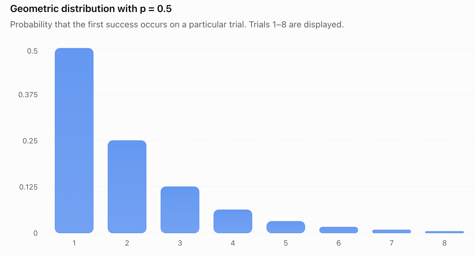
The graph shows a rapidly decreasing probability as the first success occurs later.

The probabilities continue beyond trial 8, and the sum over all possible trial numbers equals 1.

Geometric Cumulative Probabilities

Sometimes a problem asks for the probability that the first success occurs within a certain number of trials.

At Most k Trials

The probability that the first success occurs on or before trial k is:

P(X ≤ k) = 1 − (1 − p)ᵏ

This formula uses complementary probability.

The opposite event is failing on all k trials.

Worked Example: Success Within Four Attempts

A player has a 30% probability of success on each independent attempt.

Find the probability of achieving the first success within four attempts.

p = 0.3

k = 4

P(X ≤ 4) = 1 − (0.7)⁴

= 1 − 0.2401

P(X ≤ 4) = 0.7599

There is a 75.99% probability of achieving at least one success within four attempts.

More Than k Trials

The probability that more than k trials are required is:

P(X > k) = (1 − p)ᵏ

For example, if p = 0.3:

P(X > 4) = 0.7⁴

P(X > 4) = 0.2401

There is a 24.01% probability that the first four attempts all fail.

Expected Value of a Geometric Distribution

The expected value of a geometric distribution gives the average number of trials required to obtain the first success.

For the convention where X counts trials, including the successful trial:

E(X) = 1/p

Worked Example: Expected Number of Attempts

A student has a 25% probability of solving a particular type of problem correctly on each independent attempt.

Find the expected number of attempts required for the first correct answer.

p = 0.25

E(X) = 1/0.25

E(X) = 4

The expected number of attempts is four.

This does not mean the first success must occur on the fourth attempt.

It represents the long-run average number of attempts across many repetitions of the experiment.

Variance and Standard Deviation of a Geometric Distribution

For a geometric random variable counting trials until the first success:

Var(X) = (1 − p)/p²

The standard deviation is:

σ = √(1 − p)/p

Worked Example

Suppose:

p = 0.25

Expected value:

E(X) = 1/0.25 = 4

Variance:

Var(X) = 0.75/(0.25)²

= 0.75/0.0625

Var(X) = 12

Standard deviation:

σ = √12

σ ≈ 3.46

The expected number of trials is four, but the standard deviation is approximately 3.46 trials.

This indicates that the number of attempts required can vary considerably.

The Memoryless Property

One of the most interesting features of the geometric distribution is its memoryless property.

This means that previous failures do not change the probability of future success.

For a geometric random variable:

P(X > m + n | X > m) = P(X > n)

where the vertical bar means "given that."

Example: Repeated Attempts

Suppose the probability of success on each independent attempt is 0.2.

A student has already failed five times.

What is the probability of success on the next attempt?

The probability remains:

0.2

The previous failures do not change the probability of success on the next independent attempt.

The geometric distribution does not remember how many failures have already occurred.

Important Limitation

The memoryless property applies only when trials are independent and the success probability remains constant.

In real situations, learning, fatigue, equipment changes, or other factors may change the probability of success.

The Poisson Distribution

A Poisson distribution describes the number of events occurring within a fixed interval of time, space, distance, area, or another measurement.

Examples include:

• The number of customers arriving at a shop each hour.

• The number of telephone calls received per minute.

• The number of typing errors on a page.

• The number of defects in a length of material.

• The number of meteor observations during a night.

The Poisson distribution is useful when events occur randomly at a constant average rate.

Conditions for a Poisson Distribution

A Poisson model is appropriate when:

• Events are counted within a fixed interval or region.

• Events occur independently.

• The average rate of occurrence is constant across equal-sized intervals or regions.

• Events occur singly in sufficiently small intervals, with the probability of multiple events in a tiny interval becoming negligible.

These assumptions describe an idealized random event process.

Example: Telephone Calls

Suppose a call centre receives an average of four calls per minute.

If calls arrive independently and at a constant average rate, the number of calls in a minute may be modelled using a Poisson distribution.

Let:

X = number of calls received in one minute

Then:

X ~ Poisson(4)

The parameter 4 represents the expected number of calls in the interval.

Poisson Distribution Notation

A Poisson random variable is written as:

X ~ Poisson(λ)

The symbol λ (lambda) represents the average number of events in the specified interval.

For example:

X ~ Poisson(3)

means that the expected number of events in the interval is three.

The possible values are:

X = 0, 1, 2, 3, ...

Unlike the binomial distribution, there is no fixed maximum number of events in the mathematical model.

The Poisson Probability Formula

The probability of observing exactly k events is:

P(X = k) = (e^(−λ) × λᵏ)/k!

where:

• λ is the average number of events in the interval.

• k is the number of events being counted.

• e is a mathematical constant approximately equal to 2.71828.

• k! represents factorial.

For a Poisson distribution, λ must be positive and k must be a non-negative integer.

Understanding the Formula

The formula combines:

• The average event rate, λ.

• The number of observed events, k.

• The exponential factor e^(−λ).

• The factorial k!, which accounts for the event count.

It calculates the probability of observing exactly k events in the specified interval.

Worked Example: Telephone Calls

A call centre receives an average of three calls per minute.

Assume calls follow a Poisson distribution.

Find the probability of receiving exactly two calls in one minute.

Step 1: Identify the values.

λ = 3

k = 2

Step 2: Substitute into the formula.

P(X = 2) = (e^(−3) × 3²)/2!

Step 3: Simplify.

= (e^(−3) × 9)/2

Using:

e^(−3) ≈ 0.04979

P(X = 2) ≈ (0.04979 × 9)/2

Final answer:

P(X = 2) ≈ 0.2240

There is approximately a 22.40% probability of receiving exactly two calls in one minute.

Constructing a Poisson Probability Distribution

Suppose events occur at an average rate of:

λ = 2 per interval

Then:

X ~ Poisson(2)

Calculate the probabilities for several possible values.

P(X = 0) = e^(−2) ≈ 0.1353

P(X = 1) = 2e^(−2) ≈ 0.2707

P(X = 2) = (2²e^(−2))/2! ≈ 0.2707

P(X = 3) = (2³e^(−2))/3! ≈ 0.1804

P(X = 4) = (2⁴e^(−2))/4! ≈ 0.0902

These probabilities do not add to 1 because outcomes greater than four have not been included.

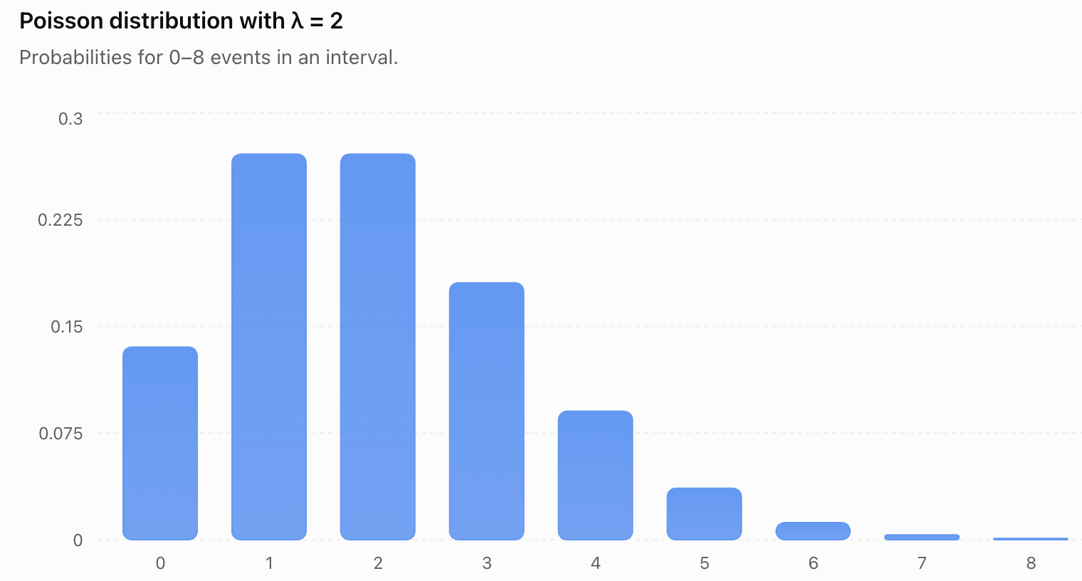
The distribution is concentrated around one and two events.

The probability decreases for larger event counts.

Expected Value and Variance of a Poisson Distribution

A useful property of the Poisson distribution is that its expected value and variance are equal.

E(X) = λ

Var(X) = λ

The standard deviation is:

σ = √λ

Worked Example

Suppose a shop receives an average of nine customers per hour, following a Poisson distribution.

λ = 9

Expected value:

E(X) = 9

Variance:

Var(X) = 9

Standard deviation:

σ = √9

σ = 3

Interpretation

The expected number of customers is nine per hour.

The standard deviation is three customers.

This describes the scale of variation in hourly customer counts under the Poisson model.

Changing the Time Interval

A Poisson model may describe events occurring at a constant average rate.

If the interval changes, the expected number of events changes proportionally.

For example, suppose a shop receives an average of six customers per hour.

Then:

• In one hour: λ = 6

• In 30 minutes: λ = 3

• In two hours: λ = 12

• In three hours: λ = 18

Worked Example: Calls in Ten Minutes

A call centre receives an average of 12 calls per hour.

Find the probability of receiving exactly three calls in ten minutes.

Step 1: Adjust λ.

Ten minutes is one-sixth of an hour.

λ = 12 × (10/60)

λ = 2

Step 2: Apply the Poisson formula.

P(X = 3) = (e^(−2) × 2³)/3!

= (e^(−2) × 8)/6

P(X = 3) ≈ 0.1804

There is approximately an 18.04% probability of receiving exactly three calls in ten minutes.

Important Reminder

Always ensure that λ corresponds to the interval stated in the question.

Using an hourly rate in a ten-minute calculation without adjustment will produce an incorrect answer.

Cumulative Poisson Probabilities

Poisson questions often ask for probabilities involving more than one possible event count.

Worked Example: At Most Two Events

Suppose:

X ~ Poisson(2)

Find:

P(X ≤ 2)

This means:

P(X = 0) + P(X = 1) + P(X = 2)

Using the values calculated earlier:

P(X ≤ 2) ≈ 0.1353 + 0.2707 + 0.2707

P(X ≤ 2) ≈ 0.6767

There is approximately a 67.67% probability of observing at most two events.

Worked Example: At Least One Event

Suppose the average number of events is:

λ = 3

Find the probability of at least one event.

Use complementary probability:

P(X ≥ 1) = 1 − P(X = 0)

P(X = 0) = e^(−3)

≈ 0.0498

Therefore:

P(X ≥ 1) = 1 − 0.0498

P(X ≥ 1) ≈ 0.9502

There is approximately a 95.02% probability of observing at least one event.

Comparing Geometric and Poisson Distributions

Although both distributions are discrete, they model different situations.

The key distinction is:

Geometric distributions count how long it takes to achieve the first success, while Poisson distributions count how many events occur in a fixed interval.

Comparing Binomial, Geometric, and Poisson Distributions

These three distributions are closely related but answer different questions.

Example: Basketball

A player makes each free throw with probability 0.7.

Binomial question:

How many successful shots occur in ten attempts?

Geometric question:

How many attempts are needed to make the first successful shot?

Example: Customer Arrivals

A shop receives customers randomly at an average rate of five per hour.

Poisson question:

How many customers arrive during the next hour?

The distribution depends on what is being counted.

The Poisson Approximation to the Binomial Distribution

The Poisson distribution can sometimes approximate a binomial distribution when:

• The number of trials n is large.

• The probability of success p is small.

• The product np is of a manageable size.

In this situation:

λ = np

Example: Rare Defects

A factory produces 1,000 components.

Each component has a 0.002 probability of being defective.

Let X represent the number of defective components.

The exact model is:

X ~ B(1000, 0.002)

Since:

n = 1000

p = 0.002

λ = np = 2

A Poisson approximation is:

X ≈ Poisson(2)

Probability of Exactly Three Defects

P(X = 3) ≈ (e^(−2) × 2³)/3!

P(X = 3) ≈ 0.1804

This approximation is useful because the Poisson formula can be easier to calculate than a binomial formula involving a very large n.

However, the approximation is not exact, and its accuracy depends on the values of n and p.

Practical Application: Manufacturing Defects

A company produces long rolls of fabric.

On average, there are two defects per 100 metres.

Assume defects occur independently at a constant average rate.

Let X represent the number of defects in 100 metres.

Then:

X ~ Poisson(2)

Probability of No Defects

P(X = 0) = e^(−2)

P(X = 0) ≈ 0.1353

There is approximately a 13.53% probability that a 100-metre roll contains no defects.

Expected Number of Defects in 250 Metres

The expected number of defects increases proportionally with length.

λ = 2 × (250/100)

λ = 5

The expected number of defects in 250 metres is five.

Practical Application: Customer Service

A customer-service centre receives an average of eight calls per hour.

Assume calls follow a Poisson process.

Probability of No Calls in 15 Minutes

First adjust the rate.

15 minutes = 0.25 hours

λ = 8 × 0.25

λ = 2

Then:

P(X = 0) = e^(−2)

P(X = 0) ≈ 0.1353

There is approximately a 13.53% probability of receiving no calls during a 15-minute period.

This information may help the centre plan staffing and workloads.

Practical Application: Repeated Testing

A student completes independent practice questions.

Each question has a 40% probability of being answered correctly.

Let X represent the number of attempts required to obtain the first correct answer.

Then:

X ~ Geometric(0.4)

Expected Number of Attempts

E(X) = 1/0.4

E(X) = 2.5

Probability of First Success on the Fourth Attempt

P(X = 4) = (0.6)³ × 0.4

= 0.216 × 0.4

P(X = 4) = 0.0864

There is an 8.64% probability that the first correct answer occurs on the fourth attempt.

This model assumes that the student's probability of answering correctly remains constant. In a real learning situation, practice may improve performance, making the model less accurate.

Selecting an Appropriate Probability Model

When solving a probability problem, begin by identifying what the random variable counts.

Decision Guide

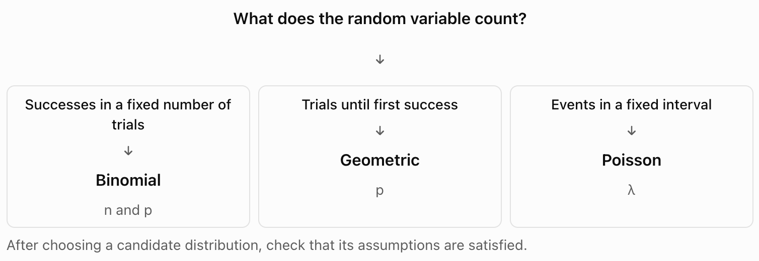
Questions to Ask

Before choosing a probability distribution, consider:

1. Is the number of trials fixed?

2. Are we counting successes or waiting for the first success?

3. Are we counting events in a time interval or region?

4. Are trials or events independent?

5. Is the success probability or average event rate constant?

The correct distribution depends on both the question and the assumptions.

Common Mistakes

Confusing geometric and binomial distributions

Binomial distributions count successes in a fixed number of trials. Geometric distributions count trials until the first success.

Using the wrong geometric formula

The formula P(X = k) = (1 − p)^(k−1)p assumes that X counts the successful trial as well as preceding failures.

Forgetting that geometric variables begin at 1

Under the trials-until-first-success convention, X cannot equal zero.

Confusing probability with average event rate

The geometric parameter p is a probability, while the Poisson parameter λ is an expected event count.

Using the wrong interval for λ

Poisson rates must be adjusted to match the interval in the question.

Forgetting factorials in the Poisson formula

The denominator k! is essential.

Confusing exactly, at most, and at least

These expressions require different probability calculations.

Forgetting complementary probability

Questions involving at least one event are often easier to solve using 1 − P(X = 0).

Assuming every event-counting situation is Poisson

The Poisson model requires appropriate independence and constant-rate assumptions.

Assuming geometric trials are always equally likely to succeed and fail

The probability of success can be any value greater than zero and at most one.

Ignoring the limitations of mathematical models

Real-world events may involve dependence, changing probabilities, or varying event rates.

Key Terms

• Geometric Distribution: A discrete probability distribution describing the number of independent trials required to obtain the first success.

• Poisson Distribution: A discrete probability distribution describing the number of events occurring in a fixed interval or region at a constant average rate.

• Binomial Distribution: A distribution describing the number of successes in a fixed number of independent trials.

• Random Variable: A variable assigning numerical values to the outcomes of a random experiment.

• Discrete Random Variable: A random variable with a finite or countably infinite set of possible values.

• Trial: One repetition of a random experiment.

• Success: The outcome of interest in a probability experiment.

• Failure: The alternative outcome to success.

• Independent Trials: Trials in which the outcome of one does not affect the probability of another.

• Constant Probability: A success probability that remains unchanged across trials.

• Probability Distribution: A description of the probabilities assigned to possible values of a random variable.

• Probability Mass Function: A function giving the probability of each possible value of a discrete random variable.

• Expected Value: The long-run average value of a random variable.

• Variance: A measure of the spread of outcomes around the expected value.

• Standard Deviation: The positive square root of variance.

• Lambda (λ): The average number of events in a specified interval for a Poisson distribution.

• Euler's Number (e): A mathematical constant approximately equal to 2.71828.

• Factorial: The product of all positive integers up to a given positive integer.

• Complementary Probability: The probability that an event does not occur.

• Cumulative Probability: The probability that a random variable falls within a specified range of values.

• Memoryless Property: The property that previous failures do not change the conditional distribution of future waiting time in a geometric model.

• Poisson Process: A mathematical model of events occurring independently at a constant average rate over time or space.

• Poisson Approximation: The use of a Poisson distribution to approximate a binomial distribution when n is large and p is small.

• Mathematical Model: A simplified mathematical representation of a real-world situation.

• Event Rate: The average number of events occurring per unit of time, distance, area, or another measurement.

Key Takeaways

• Geometric distributions describe the number of trials required to obtain the first success.

• Geometric experiments involve independent trials with a constant probability of success.

• The geometric probability formula is P(X = k) = (1 − p)^(k−1)p.

• The expected value of a geometric distribution is E(X) = 1/p.

• The variance of a geometric distribution is Var(X) = (1 − p)/p².

• Geometric distributions have the memoryless property.

• Poisson distributions describe the number of events occurring in a fixed interval or region.

• Poisson models assume events occur independently at a constant average rate.

• The Poisson probability formula is P(X = k) = (e^(−λ) × λᵏ)/k!.

• The parameter λ represents the expected number of events in the specified interval.

• For a Poisson distribution, both the expected value and variance equal λ.

• The standard deviation of a Poisson distribution is √λ.

• Poisson rates must be adjusted when the interval changes.

• Complementary probability is useful for calculating probabilities involving at least one event or success.

• The Poisson distribution can approximate a binomial distribution when n is large and p is small.

• Binomial, geometric, and Poisson distributions answer different types of probability questions.

• Choosing the correct probability model requires identifying what is counted and checking the assumptions.

• These distributions are useful in manufacturing, customer service, science, engineering, business, and everyday decision-making.

Check Your Understanding

Recall and Understanding

1. Define a geometric distribution and explain when it is appropriate.

2. State the formula for calculating geometric probabilities.

3. Define a Poisson distribution and explain the meaning of λ.

4. State the formula for calculating Poisson probabilities.

5. Explain the main differences between binomial, geometric, and Poisson distributions.

Application

6. A basketball player has a 70% probability of making each independent shot. Calculate the probability that the first successful shot occurs on the fourth attempt.

7. A student has a 20% probability of answering each independent question correctly. Calculate the expected number of attempts required for the first correct answer.

8. A call centre receives an average of four calls per minute. Assuming a Poisson model, calculate the probability of receiving exactly two calls in one minute.

9. A shop receives an average of six customers per hour. Calculate the probability of receiving no customers in a 30-minute period, assuming a Poisson process.

10. A geometric random variable has p = 0.4. Calculate its expected value, variance, and standard deviation.

Analysis and Challenge

11. A student has a 30% probability of success on each independent attempt. Calculate the probability of achieving the first success within five attempts.

12. A factory produces an average of three defects per 100 metres of material. Assuming a Poisson process, calculate the probability of finding at least one defect in 50 metres.

13. A call centre receives an average of eight calls per hour. Calculate the probability of receiving at most two calls in 15 minutes.

14. A factory produces 500 items, each with an independent defect probability of 0.004. Explain why a Poisson approximation may be appropriate and use it to estimate the probability of exactly three defective items.

15. For each of the following situations, identify the most appropriate distribution and justify your choice:

• The number of successful free throws in ten attempts.

• The number of attempts required to make the first successful free throw.

• The number of customers arriving at a shop during one hour.

Final Summary

Geometric and Poisson distributions extend our ability to model uncertain events beyond experiments involving a fixed number of trials.

The geometric distribution describes the number of attempts required to achieve the first success, while the Poisson distribution describes the number of events occurring within a fixed interval or region.

By understanding their formulas, expected values, variances, and assumptions, students can calculate probabilities and interpret the results in practical situations.

Comparing geometric, Poisson, and binomial distributions is an important step toward selecting appropriate probability models.

These concepts provide a foundation for advanced probability, statistics, scientific modelling, risk analysis, and real-world decision-making.