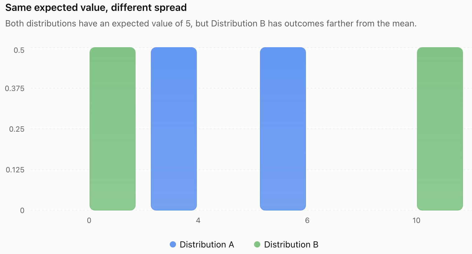
Distribution B has a much greater variance because its outcomes are farther from the mean.

This demonstrates why expected value alone does not fully describe a random variable.

Standard Deviation

The standard deviation is the positive square root of the variance.

For a random variable X:

σ = √Var(X)

where σ (sigma) represents the standard deviation.

Standard deviation measures the spread of outcomes around the mean.

Unlike variance, standard deviation is expressed in the same units as the original variable.

For example:

• If X is measured in dollars, standard deviation is measured in dollars.

• If X is measured in seconds, standard deviation is measured in seconds.

• If X is measured in metres, standard deviation is measured in metres.

Variance, by contrast, is expressed in squared units.

Worked Example: Standard Deviation

Suppose:

Var(X) = 9

Then:

σ = √9

σ = 3

If X represents the number of customers, the standard deviation is 3 customers.

Calculating Standard Deviation from a Distribution

Consider the distribution:

We previously calculated:

E(X) = 2

Var(X) = 0.5

Therefore:

σ = √0.5

σ ≈ 0.707

The standard deviation is approximately 0.71.

Interpreting the Result

The possible values are relatively close to the expected value of 2.

A standard deviation of approximately 0.71 indicates a modest spread around the mean.

Standard deviation should not be interpreted as a strict limit on how far outcomes can lie from the mean.

Comparing Standard Deviations

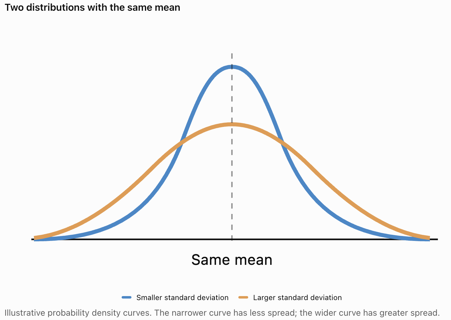
A smaller standard deviation means that values tend to cluster more closely around the mean.

A larger standard deviation means that values tend to be more widely spread.

Important Interpretation

Standard deviation describes variability, not whether an outcome is good or bad.

A high standard deviation may represent:

• Greater uncertainty.

• More variable results.

• A wider range of possible outcomes.

Whether this is desirable depends on the situation.

For example, a company may prefer consistent production quality, while a researcher may be interested in naturally variable measurements.

Variance and Standard Deviation of a Fair Die

A fair six-sided die provides a useful example.

The expected value is:

E(X) = 3.5

Calculate E(X²):

E(X²) = [1² + 2² + 3² + 4² + 5² + 6²]/6

= (1 + 4 + 9 + 16 + 25 + 36)/6

= 91/6

≈ 15.1667

Calculate variance:

Var(X) = E(X²) − [E(X)]²

= 91/6 − 3.5²

= 91/6 − 12.25

Var(X) = 35/12 ≈ 2.917

Calculate standard deviation:

σ = √(35/12)

σ ≈ 1.708

Summary

For a fair six-sided die:

• Expected value = 3.5

• Variance ≈ 2.917

• Standard deviation ≈ 1.708

These values describe both the centre and spread of the die's probability distribution.

Properties of Expected Value

Expected value follows several useful mathematical rules.

Adding a Constant

If a constant c is added to every possible value:

E(X + c) = E(X) + c

For example, if:

E(X) = 5

then:

E(X + 3) = 8

Multiplying by a Constant

If every possible value is multiplied by a constant a:

E(aX) = aE(X)

For example:

E(4X) = 4E(X)

Combining Both Operations

E(aX + b) = aE(X) + b

This rule is useful when converting units or transforming random variables.

Properties of Variance and Standard Deviation

Variance behaves differently from expected value.

Adding a Constant

Adding a constant to every outcome shifts the distribution but does not change its spread.

Var(X + c) = Var(X)

For example, if every employee receives a $100 increase in a particular payment, the variance of those payments remains unchanged.

Multiplying by a Constant

Multiplying every outcome by a constant changes the variance by the square of that constant.

Var(aX) = a²Var(X)

For example, if:

Var(X) = 4

then:

Var(3X) = 3² × 4

= 36

Standard Deviation

Standard deviation changes by the absolute value of the multiplier.

SD(aX + b) = |a|SD(X)

These properties are useful when changing measurement units or comparing transformed distributions.

Expected Value in Games and Gambling

Expected value can be used to determine whether a game is mathematically fair.

A fair game has an expected net gain of zero.

Worked Example: A Dice Game

A player pays $4 to roll a fair six-sided die.

If the player rolls a 6, they receive $18.

Otherwise, they receive nothing.

Let X represent the player's net gain.

If the player wins:

X = 18 − 4 = $14

If the player loses:

X = −$4

The probabilities are:

P(win) = 1/6

P(lose) = 5/6

Expected value:

E(X) = 14(1/6) + (−4)(5/6)

= 14/6 − 20/6

= −6/6

E(X) = −$1

Interpretation

The player loses an average of $1 per game over many repetitions.

The game is not mathematically fair to the player.

Using Expected Value for Decision-Making

Expected value is especially useful when comparing choices involving uncertain outcomes.

Worked Example: Comparing Two Projects

A business is considering two possible projects.

Project A

• 80% probability of earning $1,000

• 20% probability of losing $500

Expected value:

E(A) = 0.80(1000) + 0.20(−500)

= 800 − 100

E(A) = $700

Project B

• 50% probability of earning $1,800

• 50% probability of losing $200

Expected value:

E(B) = 0.50(1800) + 0.50(−200)

= 900 − 100

E(B) = $800

Project B has the higher expected profit.

However, we should also compare the variance and standard deviation.

Comparing Risk Using Variance

Project A

Expected value:

μ = 700

Variance:

Var(A) = (1000 − 700)²(0.80) + (−500 − 700)²(0.20)

= 300²(0.80) + (−1200)²(0.20)

= 90,000(0.80) + 1,440,000(0.20)

= 72,000 + 288,000

Var(A) = 360,000

Standard deviation:

SD(A) = √360,000

SD(A) = $600

Project B

Expected value:

μ = 800

Variance:

Var(B) = (1800 − 800)²(0.50) + (−200 − 800)²(0.50)

= 1000²(0.50) + (−1000)²(0.50)

= 500,000 + 500,000

Var(B) = 1,000,000

Standard deviation:

SD(B) = √1,000,000

SD(B) = $1,000

Comparing the Projects

Interpretation

Project B has a higher expected profit, but also greater variability.

Project A has a lower expected profit and a smaller standard deviation.

Interestingly, Project A has a larger possible loss, despite its lower variance.

This illustrates an important point:

Standard deviation measures spread, but it does not fully describe every type of risk.

A decision-maker should consider:

• Expected return.

• Variability.

• Maximum possible loss.

• Available financial resources.

• The consequences of an unfavourable outcome.

• Personal or organizational risk tolerance.

Expected Value and Insurance

Insurance provides another practical application of expected value.

Suppose an insurance company estimates that a particular type of claim has:

• A 2% probability of occurring.

• An average payout of $5,000 if it occurs.

The expected payout per policy is:

E(X) = 0.02(5000) + 0.98(0)

E(X) = $100

The expected claim cost is $100 per policy.

An insurance company must consider this expected cost, along with administrative expenses, uncertainty, reserves, and other factors when setting premiums.

Expected Value and the Binomial Distribution

The binomial distribution describes the number of successes in a fixed number of independent trials when each trial has the same probability of success.

If:

X follows a binomial distribution with parameters n and p,

then:

E(X) = np

Var(X) = np(1 − p)

SD(X) = √[np(1 − p)]

where:

• n is the number of trials.

• p is the probability of success.

• 1 − p is the probability of failure.

Worked Example: Coin Tosses

A fair coin is tossed 20 times.

Let X represent the number of heads.

n = 20

p = 0.5

Expected value:

E(X) = 20 × 0.5

E(X) = 10

Variance:

Var(X) = 20 × 0.5 × 0.5

Var(X) = 5

Standard deviation:

SD(X) = √5

SD(X) ≈ 2.236

Interpretation

The expected number of heads is 10.

The standard deviation is approximately 2.24 heads, describing the typical scale of variation around the expected number.

The actual number of heads will not necessarily be 10 in every set of 20 tosses.

Understanding Measures of Spread

Expected value, variance, and standard deviation describe different aspects of a distribution.

Small Variance and Standard Deviation

A small variance indicates that outcomes tend to be close to the expected value.

Examples include:

• Consistent manufacturing measurements.

• Predictable delivery times.

• Stable daily demand.

Large Variance and Standard Deviation

A large variance indicates that outcomes tend to be more widely spread.

Examples include:

• Highly variable sales.

• Uncertain investment returns.

• Inconsistent waiting times.

However, the meaning of "large" or "small" depends on the scale and context of the variable.

The Relationship Between Standard Deviation and Normal Distributions

Many naturally occurring measurements can be approximately modelled using a normal distribution.

A normal distribution has a symmetrical, bell-shaped curve.

For an exactly normal distribution:

• Approximately 68% of values lie within one standard deviation of the mean.

• Approximately 95% lie within two standard deviations.

• Approximately 99.7% lie within three standard deviations.

This is known as the Empirical Rule.

Example: Test Scores

Suppose test scores are approximately normally distributed with:

Mean = 70

Standard deviation = 10

Then approximately:

• 68% of scores lie between 60 and 80.

• 95% lie between 50 and 90.

• 99.7% lie between 40 and 100.

These percentages are approximate and apply to distributions that are normal or closely resemble a normal distribution.

They should not automatically be applied to every probability distribution.

Common Mistakes

Confusing expected value with the most likely outcome

Expected value is a weighted average, while the most likely outcome is the mode.

Assuming expected value must be a possible outcome

The expected value of a die is 3.5, even though a die cannot show 3.5.

Forgetting to multiply each value by its probability

Expected value is calculated using weighted values.

Calculating variance without first finding the mean

Variance measures spread around the expected value.

Forgetting to square deviations

Negative and positive deviations would otherwise cancel.

Confusing variance and standard deviation

Standard deviation is the square root of variance.

Using the wrong units

Variance has squared units, while standard deviation has the original units.

Assuming a larger expected value always means a better decision

Risk, possible losses, and other factors may also be important.

Assuming a larger variance always means a worse outcome

Greater variability may be acceptable or desirable in some situations.

Applying normal-distribution rules to every distribution

The 68–95–99.7 rule applies specifically to normal distributions.

Key Terms

• Expected Value: The probability-weighted average of the possible values of a random variable.

• Mean: The average value of a probability distribution.

• Random Variable: A variable that assigns numerical values to outcomes of a random experiment.

• Probability Distribution: A description of the probabilities associated with possible values of a random variable.

• Variance: The probability-weighted average of squared deviations from the expected value.

• Standard Deviation: The positive square root of variance.

• Deviation: The difference between an observed or possible value and the mean.

• Squared Deviation: The square of the difference between a value and the mean.

• Weighted Average: An average in which values contribute according to assigned weights.

• Spread: The extent to which values differ from one another or from the centre of a distribution.

• Variability: The degree to which outcomes differ across observations or trials.

• Risk: The possibility of outcomes that differ from expectations, particularly unfavourable outcomes.

• Fair Game: A game with an expected net gain of zero for the player.

• Long-Run Average: The average outcome approached over many repeated experiments.

• Binomial Distribution: A distribution describing the number of successes in repeated independent trials with constant success probability.

• Normal Distribution: A symmetrical, bell-shaped continuous probability distribution.

• Empirical Rule: The approximate 68–95–99.7 pattern for normal distributions.

• Risk Tolerance: The amount of uncertainty or potential loss a decision-maker is willing or able to accept.

• Probability Model: A mathematical representation of uncertain outcomes.

• Decision-Making Under Uncertainty: Choosing between alternatives when their outcomes are not known with certainty.

Key Takeaways

• Expected value describes the long-run average outcome of a random variable.

• Expected value is calculated by multiplying each possible value by its probability and adding the products.

• Variance measures the average squared distance of outcomes from the expected value.

• Standard deviation is the positive square root of variance.

• Variance is measured in squared units, while standard deviation uses the original units.

• Two distributions can have the same expected value but different variances.

• A smaller standard deviation indicates outcomes tend to cluster more closely around the mean.

• A larger standard deviation indicates greater variability.

• Expected value can be used to evaluate games, business projects, insurance, and financial decisions.

• A fair game has an expected net gain of zero.

• Expected value alone does not fully describe risk.

• Variance and standard deviation help compare uncertainty between different choices.

• For a binomial distribution, E(X) = np and Var(X) = np(1 − p).

• Adding a constant changes expected value but not variance.

• Multiplying a random variable by a constant changes variance by the square of that constant.

• The Empirical Rule describes how values are distributed around the mean in a normal distribution.

• Expected value, variance, and standard deviation are essential tools in probability, statistics, and decision-making.

Check Your Understanding

Recall and Understanding

1. Define expected value and explain what it represents.

2. State the formula for calculating the expected value of a discrete random variable.

3. Explain the difference between variance and standard deviation.

4. Why are deviations squared when calculating variance?

5. Explain why two distributions can have the same expected value but different standard deviations.

Application

6. A random variable X has values 1, 2, and 3 with probabilities 0.2, 0.5, and 0.3. Calculate E(X).

7. Using the distribution in Question 6, calculate Var(X).

8. Calculate the standard deviation of the distribution in Question 6.

9. A fair six-sided die is rolled. Calculate its expected value and variance.

10. A binomial random variable has n = 12 and p = 0.25. Calculate its expected value, variance, and standard deviation.

Analysis and Challenge

11. A game costs $5 to play. A player has a 20% chance of receiving $20 and an 80% chance of receiving nothing. Calculate the expected net gain and determine whether the game is fair.

12. Two investments have the same expected return but different standard deviations. Explain how this information could influence a decision.

13. A random variable has E(X) = 8 and Var(X) = 4. Find E(3X + 2), Var(3X + 2), and SD(3X + 2).

14. A business is considering two projects. Project A has a 70% chance of earning $1,000 and a 30% chance of losing $400. Project B has a 40% chance of earning $2,000 and a 60% chance of losing $100. Calculate the expected value of each project and discuss which might be preferable.

15. Explain why expected value and standard deviation should be considered together when making decisions under uncertainty.

Final Summary

Expected value, variance, and standard deviation are fundamental tools for analysing probability distributions.

Expected value describes the long-run average outcome, while variance and standard deviation measure how widely possible outcomes are spread around that average.

By calculating these measures, students can compare probability distributions, interpret uncertainty, and evaluate decisions involving risk.

Understanding both the expected outcome and the variability of possible results provides a more complete picture than considering the average alone.

These concepts are widely used in probability, statistics, business, finance, engineering, science, and real-world decision-making.