Random Variables

Introduction to Random Variables

Many situations involve uncertainty. We may not know how many customers will enter a shop tomorrow, how long a bus will take to arrive, or how many heads will appear when a coin is tossed several times.

Although individual outcomes may be unpredictable, mathematics allows us to describe and analyse these situations using probability.

A random variable is a variable that assigns a numerical value to each possible outcome of a random experiment.

Random variables are important because they allow us to:

• Represent uncertain outcomes using numbers.

• Distinguish between different types of data.

• Calculate the probability of different results.

• Determine expected values.

• Make predictions and informed decisions.

Random variables form an important foundation for probability distributions, statistics, risk analysis, and mathematical modelling.

Understanding Random Variables

A random experiment is a process whose outcome cannot be predicted with certainty.

Examples include:

• Tossing a coin.

• Rolling a die.

• Selecting a card from a shuffled deck.

• Measuring the lifetime of a battery.

• Recording the number of customers arriving at a shop.

A random variable assigns a number to the outcome.

Random variables are commonly represented by capital letters such as X, Y, or Z.

Example: Rolling a Die

Suppose a fair six-sided die is rolled.

Let X represent the number shown.

The possible values are:

X = 1, 2, 3, 4, 5, 6

Each value has a probability of:

P(X = x) = 1/6

The random variable X describes the numerical outcome of the experiment.

Example: Tossing Two Coins

Suppose two fair coins are tossed.

The possible outcomes are:

HH, HT, TH, TT

Let X represent the number of heads obtained.

The possible values of X are:

0, 1, 2

Notice that different outcomes can produce the same value of the random variable.

For example, HT and TH both give X = 1.

This distinction is important when constructing probability distributions.

Discrete Random Variables

A discrete random variable can take a finite or countably infinite set of possible values.

Discrete random variables usually arise from counting.

Examples include:

• The number of students absent from school.

• The number of goals scored in a football match.

• The number of defective products in a sample.

• The number of heads obtained in five coin tosses.

• The number of customers entering a shop.

Discrete random variables often take whole-number values, although this is not required.

For example, a random variable representing a financial gain or loss could take values of −$5, $0, and $10.

Worked Example: Number of Heads

Three fair coins are tossed.

Let X represent the number of heads.

The possible values are:

X = 0, 1, 2, 3

The complete sample space is:

HHH, HHT, HTH, THH, HTT, THT, TTH, TTT

There are eight equally likely outcomes.

This table is a discrete probability distribution.

Continuous Random Variables

A continuous random variable can take any real value within an interval or collection of intervals.

Continuous random variables usually arise from measurement.

Examples include:

• A person's height.

• The mass of an object.

• The time required to complete a race.

• The temperature of a liquid.

• The distance travelled by a vehicle.

• The lifetime of a battery.

For example, suppose X represents the time required to run 100 metres.

Possible values might include:

12.1 seconds

12.14 seconds

12.143 seconds

12.1437 seconds

The time can theoretically take infinitely many values within a range.

Important Distinction

A continuous random variable is not limited to the precision of the measuring instrument.

A stopwatch may display times to two decimal places, but the underlying time remains continuous.

Discrete Versus Continuous Variables

Probability Distributions

A probability distribution describes how probabilities are assigned to the possible values of a random variable.

It answers questions such as:

• Which outcomes are most likely?

• Which outcomes are least likely?

• What is the probability of a particular result?

• How are the possible values distributed?

For a discrete random variable, a probability distribution can be represented using a table, graph, or formula.

Rules for a Discrete Probability Distribution

A valid discrete probability distribution must satisfy two conditions.

Every probability must be between 0 and 1.

0 ≤ P(X = x) ≤ 1

The probabilities of all possible values must add to 1.

ΣP(X = x) = 1

These conditions ensure that the distribution represents all possible outcomes correctly.

Constructing a Probability Distribution

Worked Example: Rolling a Fair Die

Let X represent the number shown when a fair six-sided die is rolled.

Check the total probability:

6 × 1/6 = 1

Therefore, the distribution is valid.

Worked Example: Two Coin Tosses

Let X represent the number of heads obtained when two fair coins are tossed.

The sample space is:

HH, HT, TH, TT

Each outcome has probability 1/4.

Simplifying:

Check:

0.25 + 0.50 + 0.25 = 1

This is a valid probability distribution.

Representing Probability Distributions Graphically

Discrete probability distributions are often displayed using bar charts.

Each bar represents the probability of a particular value.

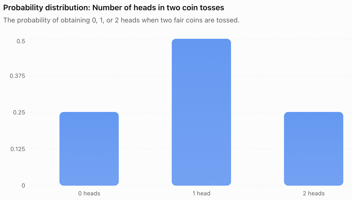
The graph shows that:

• Obtaining one head is the most likely result.

• Obtaining zero heads and two heads are equally likely.

• The probabilities add to 1.

A probability distribution provides more information than a simple list of possible values because it shows how likely each value is.

Calculating Probabilities from a Distribution

Once a probability distribution is known, probabilities involving several values can be calculated.

Suppose a random variable X has the following distribution:

Example: Find P(X = 2)

From the table:

P(X = 2) = 0.40

Example: Find P(X ≥ 2)

The symbol ≥ means greater than or equal to.

P(X ≥ 2) = P(X = 2) + P(X = 3)

= 0.40 + 0.25

P(X ≥ 2) = 0.65

Example: Find P(X < 2)

P(X < 2) = P(X = 0) + P(X = 1)

= 0.10 + 0.25

P(X < 2) = 0.35

Example: Find P(X ≠ 0)

Using complementary probability:

P(X ≠ 0) = 1 − P(X = 0)

= 1 − 0.10

P(X ≠ 0) = 0.90

Expected Value

The expected value of a random variable is the probability-weighted average of its possible values.

It describes the long-run average result that would be obtained if the random experiment were repeated many times under the same conditions.

Expected value is also called the mean of a probability distribution.

The expected value of a discrete random variable X is:

E(X) = ΣxP(X = x)

This means:

1. Multiply each possible value by its probability.

2. Add the resulting products.

Worked Example: Expected Value of a Die

A fair six-sided die is rolled.

Let X represent the number shown.

Each outcome has probability 1/6.

E(X) = 1(1/6) + 2(1/6) + 3(1/6) + 4(1/6) + 5(1/6) + 6(1/6)

= (1 + 2 + 3 + 4 + 5 + 6)/6

= 21/6

E(X) = 3.5

Interpreting the Result

The expected value is 3.5, even though a die cannot show 3.5.

This is not a mistake.

Expected value represents the average result over many rolls, not necessarily a value that can occur in one experiment.

Expected Value from a Probability Table

Worked Example: Number of Customers

A small shop records the number of customers arriving during a particular five-minute period.

Let X represent the number of customers.

Calculate the expected number of customers.

Step 1: Multiply each value by its probability.

Step 2: Add the products.

E(X) = 0 + 0.20 + 0.80 + 0.60 + 0.40

E(X) = 2

Final answer:

The expected number of customers is 2 per five-minute period.

This does not mean exactly two customers will arrive every time. It describes the long-run average.

Expected Value in Games

Expected value is useful when evaluating games involving money, prizes, or risk.

Worked Example: A Prize Game

A game costs $3 to play.

A player rolls a fair six-sided die.

• Rolling a 6 wins a $12 prize.

• Rolling any other number wins nothing.

Let X represent the player's net gain.

The possible outcomes are:

• Win: $12 − $3 = $9

• Lose: $0 − $3 = −$3

The probabilities are:

P(win) = 1/6

P(lose) = 5/6

Expected value:

E(X) = 9(1/6) + (−3)(5/6)

= 9/6 − 15/6

= −6/6

E(X) = −$1

Interpreting the Result

The player loses an average of $1 per game in the long run.

The negative expected value indicates that the game favours the organizer.

A game with an expected net gain of zero is called a fair game in the mathematical sense.

Expected Value and Decision-Making

Expected value can help compare uncertain choices.

Suppose a business is considering two projects.

Project A

• 70% probability of earning $1,000

• 30% probability of losing $200

Expected value:

E(A) = 0.70(1000) + 0.30(−200)

= 700 − 60

E(A) = $640

Project B

• 50% probability of earning $1,500

• 50% probability of losing $100

Expected value:

E(B) = 0.50(1500) + 0.50(−100)

= 750 − 50

E(B) = $700

Project B has the higher expected monetary value.

However, expected value is not the only consideration. Project B also has a greater possible loss? No: its stated loss is smaller, but its outcome variability and uncertainty differ. Decision-makers should also consider risk, available resources, and the consequences of different outcomes.

Missing Probabilities

Sometimes a probability distribution contains an unknown probability.

Because all probabilities must add to 1, the missing value can be calculated.

Worked Example

Suppose X has the following distribution:

Find k.

The probabilities must add to 1:

0.15 + 0.30 + k + 0.20 = 1

0.65 + k = 1

k = 1 − 0.65

k = 0.35

The completed distribution is:

Probability Distributions for Continuous Variables

Continuous random variables are described using probability density functions.

Unlike discrete probability distributions, probabilities are associated with intervals rather than individual exact values.

For a continuous random variable:

P(X = a) = 0

for any exact value a, provided the distribution is continuous.

This does not mean that the value is impossible. It means that a single point has zero probability within a continuous range.

Example: Waiting Time

Suppose X represents the waiting time for a bus.

The waiting time might be:

• 2.5 minutes

• 2.53 minutes

• 2.537 minutes

• 2.5374 minutes

The probability of waiting exactly 2.500000... minutes is zero in a continuous model.

However, the probability of waiting between 2 and 3 minutes can be positive.

Probability as Area

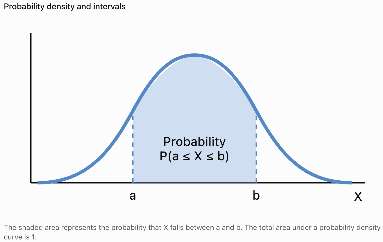
For continuous distributions, probability is represented by the area under a probability density curve.

The total area under the curve equals 1.

The Uniform Distribution

A uniform distribution describes a situation where all outcomes within a specified range are equally likely in the appropriate sense.

For a continuous uniform distribution between a and b, the probability density is constant.

Worked Example: Random Waiting Time

Suppose a bus arrives at a uniformly random time between 0 and 10 minutes after a passenger arrives.

Let X represent the waiting time.

What is the probability that the passenger waits less than 4 minutes?

For a uniform distribution:

P(X < 4) = Length of favourable interval / Total interval length

= 4/10

P(X < 4) = 0.40

There is a 40% probability of waiting less than four minutes.

Expected Value of a Continuous Uniform Distribution

For X uniformly distributed between a and b:

E(X) = (a + b)/2

For the waiting-time example:

E(X) = (0 + 10)/2

E(X) = 5 minutes

The expected waiting time is five minutes.

The Binomial Distribution

The binomial distribution describes the number of successes in a fixed number of independent trials when each trial has the same probability of success.

Examples include:

• The number of heads in ten coin tosses.

• The number of defective items in a sample.

• The number of successful attempts in a series of trials.

The binomial probability formula is:

P(X = r) = C(n, r)pʳ(1 − p)^(n−r)

where:

• n is the number of trials.

• r is the number of successes.

• p is the probability of success on each trial.

Worked Example: Three Coin Tosses

A fair coin is tossed three times.

Find the probability of obtaining exactly two heads.

n = 3

r = 2

p = 0.5

P(X = 2) = C(3, 2)(0.5)²(0.5)¹

= 3 × 0.25 × 0.5

P(X = 2) = 0.375

There is a 37.5% probability of obtaining exactly two heads.

Expected Value of a Binomial Random Variable

For a binomial random variable:

E(X) = np

For ten fair coin tosses:

n = 10

p = 0.5

E(X) = 10 × 0.5

E(X) = 5 heads

The expected number of heads is five.

Interpreting Random Variables in Context

Random variables are useful because they connect mathematical probability to real situations.

However, numerical results must be interpreted carefully.

Example: School Attendance

Let X represent the number of absent students in a class on a particular day.

If:

E(X) = 2.4

this means the long-run average number of absent students is 2.4.

It does not mean exactly 2.4 students can be absent on one day.

Example: Product Defects

Let X represent the number of defective products in a batch.

A probability distribution can help a company estimate:

• The probability of finding no defective products.

• The probability of finding more than five defective products.

• The expected number of defective products.

Example: Travel Time

Let X represent the time required to travel to school.

The probability distribution can help estimate:

• The likelihood of arriving within 20 minutes.

• The chance of a journey taking longer than 30 minutes.

• The expected travel time.

Random Variables and Mathematical Modelling

A mathematical model uses equations and probability distributions to represent a real situation.

For example, a school may model the number of students arriving late each morning.

The model could be used to estimate the probability that more than ten students arrive late.

However, mathematical models depend on assumptions.

Important questions include:

• Are the outcomes independent?

• Are the probabilities constant?

• Is the sample representative?

• Does the distribution match the observed data?

• Are there external factors that affect the results?

A probability model is useful only when its assumptions reasonably represent the situation being studied.

Common Mistakes

Confusing a random variable with an outcome

A random variable assigns a numerical value to an outcome. Different outcomes may produce the same value.

Assuming all random variables are discrete

Random variables may be discrete or continuous.

Assuming discrete variables must always be whole numbers

Discrete variables can take any finite or countably infinite set of numerical values.

Forgetting that probabilities must add to 1

A valid discrete probability distribution must have total probability equal to 1.

Using negative probabilities

Probabilities must always lie between 0 and 1.

Confusing expected value with the most likely value

The expected value is a weighted average, while the most likely value is called the mode.

Assuming expected value must be a possible outcome

A fair die has expected value 3.5, even though 3.5 cannot appear on the die.

Forgetting to multiply values by probabilities

Expected value is calculated using ΣxP(X = x), not by simply adding the possible values.

Treating probability density as probability

For continuous random variables, probabilities are found from areas under a density curve.

Ignoring context

An expected value should always be interpreted using the appropriate units and real-world meaning.

Key Terms

• Random Variable: A variable that assigns a numerical value to each outcome of a random experiment.

• Random Experiment: A process whose outcome cannot be predicted with certainty.

• Sample Space: The set of all possible outcomes of a random experiment.

• Outcome: A possible result of an experiment.

• Discrete Random Variable: A random variable with a finite or countably infinite set of possible values.

• Continuous Random Variable: A random variable that can take values across a continuous interval or collection of intervals.

• Probability Distribution: A description of how probabilities are assigned to the possible values of a random variable.

• Probability Mass Function: A function giving the probability of each possible value of a discrete random variable.

• Probability Density Function: A function describing a continuous distribution, where probabilities are determined from areas under the curve.

• Expected Value: The probability-weighted average of a random variable's possible values.

• Mean: The average value of a distribution.

• Mode: The most likely value of a discrete random variable, or a value where a density reaches a maximum in a continuous distribution.

• Uniform Distribution: A distribution with equal probabilities for discrete outcomes or constant density over a continuous interval.

• Binomial Distribution: A distribution describing the number of successes in a fixed number of independent trials with constant success probability.

• Independent Trials: Trials in which the outcome of one does not affect the probability distribution of another.

• Success Probability: The probability of the outcome designated as a success.

• Complementary Probability: The probability of an event not occurring.

• Probability Model: A mathematical representation of uncertainty in a situation.

• Long-Run Average: The average outcome approached over many repeated experiments under consistent conditions.

• Fair Game: A game with an expected net gain of zero for the player.

Key Takeaways

• A random variable assigns numerical values to the outcomes of a random experiment.

• Random variables allow uncertain situations to be analysed mathematically.

• Discrete random variables have finite or countably infinite possible values.

• Continuous random variables can take values across continuous intervals.

• Discrete random variables are often associated with counting, while continuous random variables are often associated with measurement.

• A probability distribution describes the probabilities associated with the values of a random variable.

• In a valid discrete probability distribution, every probability lies between 0 and 1 and all probabilities sum to 1.

• The expected value of a discrete random variable is calculated using E(X) = ΣxP(X = x).

• Expected value represents a long-run average, not necessarily an outcome that can occur in one experiment.

• A negative expected monetary value indicates an average loss over repeated trials.

• Continuous random variables are described using probability density functions.

• Probabilities for continuous random variables are represented by areas under density curves.

• The binomial distribution models the number of successes in repeated independent trials with constant success probability.

• Random variables are useful in education, business, science, engineering, finance, and everyday decision-making.

• Probability models must be interpreted carefully and evaluated according to their assumptions.

Check Your Understanding

Recall and Understanding

1. Define a random variable and give an example.

2. Explain the difference between discrete and continuous random variables.

3. State the two conditions required for a valid discrete probability distribution.

4. Define expected value and explain what it represents.

5. Explain why the expected value of a random variable does not always correspond to a possible outcome.

Application

6. A fair six-sided die is rolled. Let X represent the number shown. Construct the probability distribution of X.

7. Two fair coins are tossed. Let X represent the number of heads. Construct the probability distribution.

8. A random variable has values 1, 2, and 3 with probabilities 0.2, 0.5, and 0.3. Calculate E(X).

9. A probability distribution contains probabilities 0.15, 0.25, k, and 0.20. Find k.

10. A game costs $2 to play. A player has a 25% chance of receiving a $10 prize and a 75% chance of receiving nothing. Calculate the expected net gain.

Analysis and Challenge

11. Explain why the number of students in a classroom is discrete while their heights are continuous.

12. A shop records the number of customers arriving in a five-minute period. The probabilities for 0, 1, 2, and 3 customers are 0.1, 0.3, 0.4, and 0.2. Calculate the expected number of customers.

13. A fair coin is tossed five times. Use the binomial distribution to calculate the probability of obtaining exactly three heads.

14. A continuous random variable is uniformly distributed between 2 and 12. Calculate the probability that X is greater than 8 and determine E(X).

15. A business is choosing between two projects with different possible profits and losses. Explain how expected value can help compare the projects and why it should not be the only consideration.

Final Summary

Random variables provide a mathematical way to describe uncertain outcomes using numerical values.

By distinguishing between discrete and continuous random variables, students can select appropriate probability models and interpret different types of data.

Probability distributions describe how likely different outcomes are, while expected values provide a measure of the long-run average result.

These concepts form an essential foundation for probability theory, statistics, mathematical modelling, risk assessment, and informed decision-making in real-world situations.