Regression, Correlation, and Statistical Modelling
4. Statistical Modelling
Learning outcomes
- I can develop statistical models.
- I can assess model assumptions.
- I can evaluate model performance.
- I can interpret model outputs.
- I can apply models to real-world situations.
Introduction
How do scientists predict tomorrow's temperature? How do businesses estimate future sales? How can researchers investigate the factors that influence examination scores, disease rates, or population growth?
All these questions involve statistical modelling.
A statistical model is a mathematical representation of patterns and relationships in data. It allows us to describe observed behaviour, investigate relationships between variables, estimate unknown quantities, and make predictions.
Unlike a purely deterministic mathematical formula, a statistical model recognises that real-world data contain variation and uncertainty. Two students who study for the same number of hours may receive different examination scores. Two houses with similar characteristics may sell for different prices.
Statistical models help us understand these differences while identifying useful patterns.
In this lesson, we will explore how to develop statistical models, assess their assumptions, evaluate their performance, interpret their outputs, and apply them to real-world problems.
What Is a Statistical Model?
A statistical model is a mathematical description of how one or more variables are related, often including a component representing random variation.
A simple statistical model can be written as:
Where:
-
Y = observed response variable
-
X = explanatory variable
-
f(X) = systematic relationship between the variables
-
ε = random error or unexplained variation
For example, examination scores may be related to study time.
A possible model is:
This suggests that the expected examination score increases by 8 percentage points for each additional hour of study, within the range where the model is appropriate.
The error term accounts for other influences such as sleep, motivation, previous knowledge, and random variation.
Why do we use statistical models?
Statistical models can serve several purposes.
-
Description: Summarising patterns in a dataset.
-
Explanation: Investigating relationships among variables.
-
Prediction: Estimating future or unknown outcomes.
-
Inference: Drawing conclusions about a population from sample data.
-
Decision-making: Using evidence to compare possible actions.
A model designed for prediction may differ from one designed to estimate causal effects.
Developing a Statistical Model
Statistical modelling involves several connected stages.
The statistical modelling process
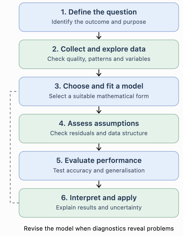
The process is iterative. Researchers often return to earlier stages after discovering problems with their data or model.
Step 1: Define the research question
Begin by identifying the outcome you want to explain or predict.
Example:
"Can examination scores be predicted using the number of hours students study?"
The response variable is examination score, and the explanatory variable is study time.
Step 2: Collect and explore data
Data should be relevant, sufficiently representative, and measured consistently.
Before fitting a model, examine:
-
Missing values and possible recording errors.
-
Unusual observations and outliers.
-
Relationships between variables.
-
Whether the data represent the intended population.
-
Whether the observations are independent or grouped.
Step 3: Choose a suitable model
The model should reflect the type of outcome and the observed pattern.
A straight-line relationship may be appropriate for some datasets, while others require nonlinear or categorical models.
Step 4: Estimate model parameters
Model parameters are numerical values that describe the relationship.
For linear regression, these include the intercept and slope.
They are estimated from data, often using the method of least squares.
Step 5: Check assumptions and performance
A model must be evaluated rather than accepted simply because it produces an equation.
Step 6: Interpret and communicate results
Explain the model in context, including its limitations and uncertainty.
Simple Linear Regression
One of the most common statistical models is simple linear regression.
It models a numerical response using one explanatory variable.
The fitted equation is:
Where:
-
ŷ = predicted response
-
a = intercept
-
b = slope
-
x = explanatory variable
Worked Example: Study Time and Examination Scores
Suppose five students produce the following data.
|
Study hours (x) |
Examination score |
|---|---|
|
1 |
48 |
|
2 |
55 |
|
3 |
61 |
|
4 |
70 |
|
5 |
76 |
We want to develop a linear model predicting examination scores from study time.
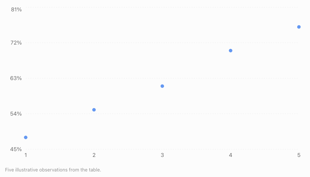
The data show a strong positive, approximately linear relationship.
Calculating the regression line
The least-squares slope is:
First calculate the means.
Now calculate the required quantities.
|
x |
y |
x − 3 |
y − 62 |
Product |
(x − 3)² |
|---|---|---|---|---|---|
|
1 |
48 |
−2 |
−14 |
28 |
4 |
|
2 |
55 |
−1 |
−7 |
7 |
1 |
|
3 |
61 |
0 |
−1 |
0 |
0 |
|
4 |
70 |
1 |
8 |
8 |
1 |
|
5 |
76 |
2 |
14 |
28 |
4 |
|
Total |
71 |
10 |
Therefore:
The intercept is:
Our fitted regression equation is:
Interpreting the model
The slope of 7.1 indicates that each additional study hour is associated with an increase of approximately 7.1 percentage points in the predicted examination score.
The intercept of 40.7 represents the predicted score at zero study hours. Because zero hours lies outside the observed range, this interpretation should be treated cautiously.
Making a prediction
For a student who studies for 4.5 hours:
The model predicts an examination score of approximately 72.7%.
This is an estimate, not a guarantee.
Choosing Different Types of Statistical Models
Different datasets require different modelling approaches.
|
Model |
Appropriate use |
Example |
|---|---|---|
|
Simple linear regression |
One numerical predictor and a numerical response |
Study time and examination score |
|
Multiple linear regression |
Several predictors and a numerical response |
House price based on size, age and location |
|
Polynomial regression |
Curved numerical relationships |
Distance travelled over time under constant acceleration |
|
Exponential regression |
Approximately constant percentage growth or decay |
Population growth |
|
Logistic regression |
Binary response |
Whether a customer makes a purchase |
|
Poisson regression |
Counts of events |
Number of calls arriving per hour |
|
Time-series model |
Data observed sequentially over time |
Monthly electricity demand |
Model selection depends on the research question, variable types, data structure, and assumptions.
Nonlinear Statistical Models
Not all relationships can be described accurately using straight lines.
Quadratic models
A quadratic model has the form:
It may describe relationships that curve upward or downward.
For example, the distance travelled by an accelerating object may follow a quadratic relationship with time.
Exponential models
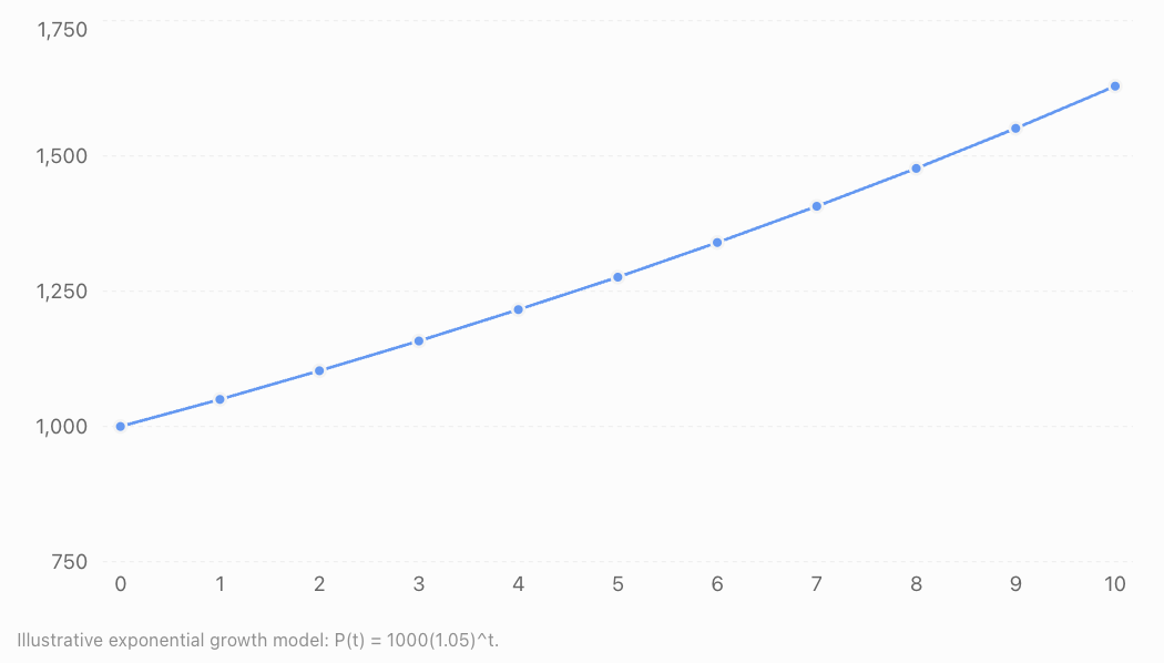
An exponential model can be written as:
Where a is the initial predicted value and b is the multiplicative factor per unit increase in x.
If b is greater than 1, the model represents exponential growth.
If b is between 0 and 1, it represents exponential decay.
Example: Population Growth
Suppose a population initially contains 1,000 organisms and increases by approximately 5% each year.
A possible model is:
After 4 years:
The predicted population is approximately 1,216 organisms.
This assumes the 5% annual growth rate remains appropriate throughout the prediction period.
Assessing Model Assumptions
Every statistical model relies on assumptions.
If important assumptions are violated, predictions, coefficient estimates, or statistical conclusions may become unreliable.
For ordinary linear regression, several assumptions deserve particular attention.
Linearity
The expected response should have an approximately linear relationship with the explanatory variables as represented in the model.
A residual plot showing a systematic curve may suggest that the model needs nonlinear terms.
Independence
Observations or errors should satisfy the independence assumptions required by the analysis.
For example, examination scores from students in the same classroom may be related because they share a teacher and learning environment.
Ignoring this grouping can produce misleading uncertainty estimates.
Constant error variance
In standard linear regression, the spread of errors is assumed to be approximately constant across fitted values.
This is called homoscedasticity.
If the spread increases or decreases systematically, the errors exhibit heteroscedasticity.
Normality of errors
For classical small-sample regression inference, errors are commonly assumed to be normally distributed.
Normality is not required simply to calculate least-squares coefficients, and it is not the same as requiring the observed response variable itself to be normally distributed.
Multicollinearity
In multiple regression, explanatory variables should not be perfectly linearly dependent.
Strong multicollinearity can make individual coefficient estimates unstable.
Model specification
The model should include an appropriate functional form and relevant explanatory information.
Omitting important variables, using inappropriate transformations, or ignoring interactions may weaken a model.
Using Residual Plots to Assess Assumptions
A residual is the difference between an observed response and the model's prediction.
Residual plots help identify patterns that may indicate model problems.
Example A: Residuals randomly scattered around zero
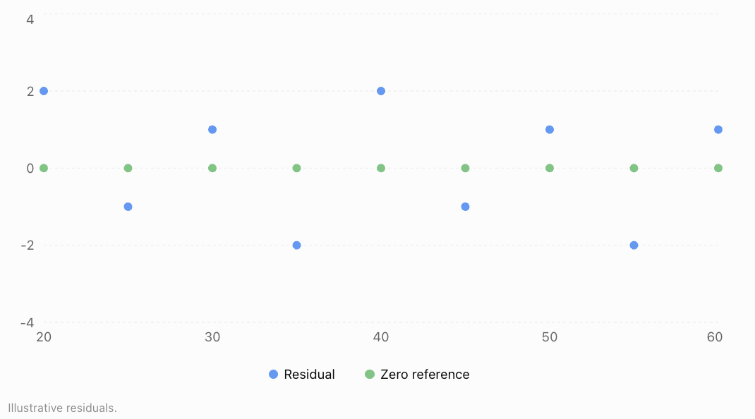
No obvious systematic pattern is visible. This is encouraging, although it does not prove that all assumptions are satisfied.
Example B: Curved residual pattern
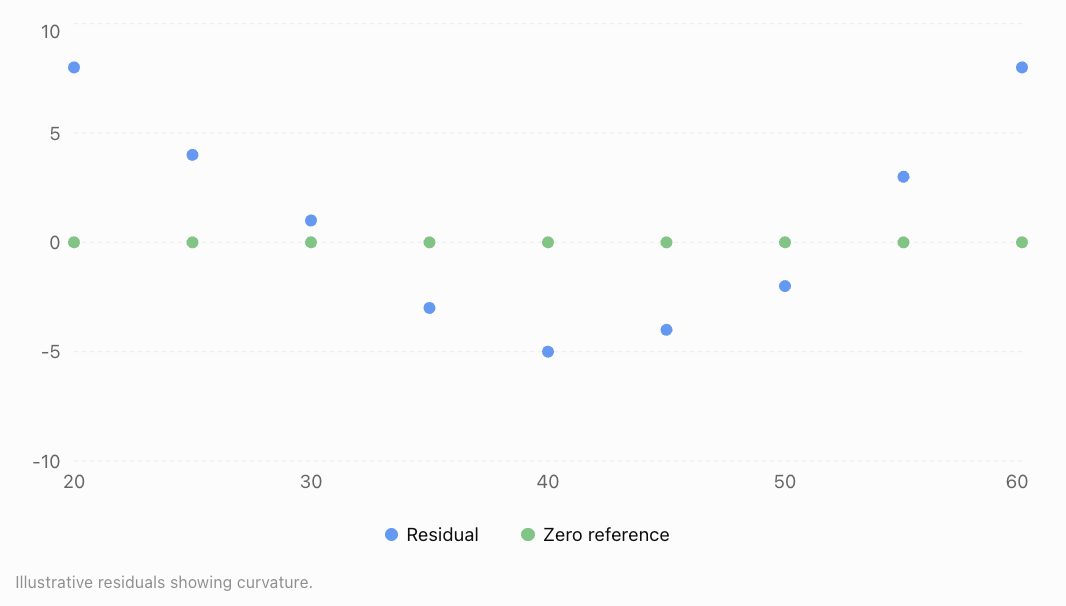
Residual plots can also show a funnel-shaped spread, suggesting nonconstant error variance.
When assumptions appear questionable, researchers may revise the model, use transformations, adopt robust inference methods, or select a different model family.
Evaluating Model Performance
A model should be judged by how well it meets its intended purpose.
For prediction, performance on previously unseen data is especially important.
Mean Absolute Error (MAE)
MAE measures the average absolute difference between observed and predicted values.
Lower values indicate smaller average absolute prediction errors.
Mean Squared Error (MSE)
MSE averages squared prediction errors.
Squaring gives greater weight to large errors.
Root Mean Squared Error (RMSE)
RMSE is the square root of MSE.
RMSE is expressed in the same units as the response variable.
Coefficient of Determination (R²)
For ordinary least-squares regression with an intercept:
Where:
-
SSres = sum of squared residuals
-
SStot = total sum of squared deviations from the observed mean
On the training dataset, R² indicates the proportion of variation explained by the model under this definition.
An R² of 0.90 means that 90% of the observed variation is accounted for by the fitted model, not that its predictions are 90% accurate.
R² on a separate test dataset can be negative when predictions perform worse than the test-set mean benchmark.
Worked Example: Calculating Prediction Errors
Suppose a model produces the following predictions.
|
Observation |
Actual |
Predicted |
Error |
Absolute error |
Squared error |
|---|---|---|---|---|---|
|
A |
50 |
52 |
−2 |
2 |
4 |
|
B |
60 |
57 |
3 |
3 |
9 |
|
C |
70 |
74 |
−4 |
4 |
16 |
|
D |
80 |
78 |
2 |
2 |
4 |
|
E |
90 |
89 |
1 |
1 |
1 |
|
Total |
12 |
34 |
Calculate MAE.
Calculate MSE.
Calculate RMSE.
The model's average absolute error is 2.4 units, while its root mean squared error is approximately 2.61 units.
RMSE is slightly larger because it gives greater weight to larger errors.
Training Data, Test Data, and Overfitting
A model may perform extremely well on the data used to build it but poorly on new observations.
This problem is called overfitting.
Training data
Training data are used to estimate model parameters.
Validation data
Validation data may be used to compare models and select settings.
Test data
Test data are held aside to provide a final assessment of predictive performance.
Example data partition

Underfitting and overfitting
Underfitting occurs when a model is too simple to capture important relationships.
Overfitting occurs when a model captures random fluctuations in training data rather than patterns that generalise.
An appropriate model balances complexity with predictive reliability.
Interpreting Model Outputs
A statistical model produces more than predictions.
It may provide coefficients, standard errors, confidence intervals, statistical tests, and measures of fit.
Consider a hypothetical multiple regression model predicting house prices in thousands of dollars.
Where:
-
A = floor area in square metres
-
G = age of the house in years
-
P = price in thousands of dollars
Interpreting coefficients
The coefficient 4.5 suggests that an additional square metre of floor area is associated with a predicted price increase of $4,500, holding house age constant.
The coefficient −1.2 suggests that each additional year of age is associated with a predicted price decrease of $1,200, holding floor area constant.
The intercept of 80 represents a predicted price of $80,000 for a property with zero floor area and zero age. This is not a realistic property, so the intercept has little practical meaning.
Worked Example: Predicting a House Price
Suppose a house has an area of 120 m² and is 15 years old.
Because the price is measured in thousands of dollars:
This prediction assumes the model is appropriate for houses with these characteristics.
Confidence intervals and prediction intervals
A confidence interval for the mean response estimates the average outcome for observations with particular explanatory-variable values.
A prediction interval estimates a range for a single new observation.
Prediction intervals are generally wider because individual outcomes contain additional variation.
For example, a model might predict a house price of $602,000, with a 95% prediction interval of $540,000 to $664,000.
The interval communicates uncertainty, although its precise interpretation depends on the statistical assumptions and method used.
Real-World Applications of Statistical Modelling
Weather Forecasting
Statistical models use historical and current atmospheric data to estimate temperatures, rainfall probabilities, and other weather conditions. Forecasts include uncertainty because atmospheric systems are complex.
Transport and Traffic
Traffic models use vehicle counts, road capacity, time of day, and weather to predict congestion and support transport planning.
Agriculture
Crop yield models investigate rainfall, soil nutrients, sunlight, temperature, and irrigation to estimate harvests and support agricultural decisions.
Business and Economics
Businesses use statistical models to forecast demand, estimate sales, investigate pricing relationships, and plan inventory.
Evaluating Whether a Model Is Appropriate
A model can have excellent numerical performance while still being unsuitable for its intended purpose.
Consider these questions:
-
Does the model answer the research question? A model that predicts accurately may not explain why a relationship occurs.
-
Are the data representative? A model trained on one population may not work for another.
-
Are important variables missing? Omitted factors may bias interpretations.
-
Are predictions being made within the observed range? Extrapolation can be unreliable.
-
Are the assumptions reasonable? Violations may affect estimates and uncertainty.
-
Does the model perform well on new data? Training performance alone is insufficient.
-
Are uncertainty and limitations communicated? Predictions should not be presented as guaranteed outcomes.
A model is useful when it is appropriate for the data, performs adequately for its purpose, and supports conclusions that can be justified.
Common Mistakes
Mistake 1: Choosing a model only because it produces a high R²
A model may fit the training data well while performing poorly on new data.
Correction: Evaluate out-of-sample performance and examine residuals.
Mistake 2: Ignoring model assumptions
A regression equation may produce misleading inferences if its assumptions are seriously violated.
Correction: Check residual patterns, independence, error variance, and other relevant assumptions.
Mistake 3: Assuming a model proves causation
Regression coefficients usually describe associations, not necessarily causal effects.
Correction: Consider study design, confounding variables, and alternative explanations.
Mistake 4: Extrapolating too far
A model developed using temperatures between 10°C and 30°C may be unreliable when predicting outcomes at 60°C.
Correction: Restrict predictions to reasonable ranges supported by the data.
Mistake 5: Confusing confidence intervals with prediction intervals
A confidence interval for the mean response is not the same as an interval for an individual future observation.
Correction: Identify the quantity whose uncertainty is being estimated.
Mistake 6: Treating predictions as exact values
Real-world observations contain unexplained variation.
Correction: Communicate prediction uncertainty and avoid unnecessary precision.
Mistake 7: Ignoring changes over time
A model based on historical conditions may become inaccurate when the underlying relationships change.
Correction: Monitor model performance and update models when appropriate.
Key Terms
-
Statistical Model: A mathematical representation of relationships and variation in data.
-
Response Variable: The outcome being explained or predicted.
-
Explanatory Variable: A variable used to explain or predict an outcome.
-
Parameter: A numerical quantity describing a statistical model.
-
Linear Regression: A method for modelling a numerical response using a linear relationship.
-
Multiple Regression: Regression involving more than one explanatory variable.
-
Nonlinear Model: A model describing relationships that are not linear in the relevant predictors or parameters.
-
Least Squares: A method that estimates parameters by minimising the sum of squared residuals.
-
Residual: The difference between an observed and predicted value.
-
Model Assumption: A condition underlying a statistical method or interpretation.
-
Homoscedasticity: Approximately constant error variance.
-
Heteroscedasticity: Nonconstant error variance.
-
MAE: Mean Absolute Error.
-
MSE: Mean Squared Error.
-
RMSE: Root Mean Squared Error.
-
R²: Coefficient of determination.
-
Training Data: Data used to fit a model.
-
Validation Data: Data used to compare or tune models.
-
Test Data: Data held aside for final predictive evaluation.
-
Overfitting: Learning random training-data fluctuations that do not generalise.
-
Underfitting: Failing to capture important relationships because a model is too simple or restrictive.
-
Cross-Validation: A technique that evaluates models across multiple training and validation splits.
-
Confidence Interval: An interval procedure used to estimate an unknown parameter or mean response with a stated confidence level.
-
Prediction Interval: An interval estimating the range of a future observation.
-
Extrapolation: Prediction beyond the range of observed data.
Key Takeaways
-
Statistical models represent patterns and relationships while accounting for uncertainty.
-
Model development begins with a clear research question and suitable data.
-
Different types of relationships require different statistical models.
-
Linear regression models numerical outcomes using linear combinations of explanatory variables.
-
Model assumptions must be examined before relying on statistical conclusions.
-
Residual plots help identify curvature, unequal error variance, and unusual observations.
-
MAE, MSE, RMSE, and R² provide different information about model performance.
-
Models should be evaluated using data not used to fit them.
-
Overfitting can produce excellent training results but poor predictions on new data.
-
Model coefficients must be interpreted in context.
-
Confidence intervals and prediction intervals describe different forms of uncertainty.
-
Statistical models support decisions but do not automatically establish causation.
Check Your Understanding
Questions
Question 1: Understanding Models
Explain what a statistical model is and why statistical models include uncertainty.
Question 2: Identifying Variables
A researcher develops a model predicting electricity consumption using outdoor temperature, household size, and the number of electrical appliances.
Identify the response variable and the explanatory variables.
Question 3: Linear Regression
A model predicts examination scores using:
Calculate the predicted score for a student who studies for 5 hours.
Question 4: Interpreting a Slope
Explain what the slope of 9 means in the model from Question 3.
Question 5: Residuals
A model predicts a house price of $450,000, but the actual selling price is $470,000.
Calculate the residual and interpret it.
Question 6: Model Performance
A model produces absolute prediction errors of 2, 4, 3, 5, and 1.
Calculate the Mean Absolute Error.
Question 7: RMSE
A model produces prediction errors of −2, 3, and −4.
Calculate the RMSE.
Question 8: Model Assumptions
A residual plot shows a clear U-shaped pattern.
What does this suggest about the model?
Question 9: Overfitting
A model achieves R² = 0.98 on its training data but R² = 0.35 on its test data.
Explain what this may indicate.
Question 10: Model Selection
A researcher wants to predict whether a student will pass or fail an examination using attendance and study time.
Which type of model would be suitable, and why?
Question 11: Exponential Modelling
A population begins with 500 organisms and grows by 8% annually.
Write an exponential model and predict the population after 3 years.
Question 12: Statistical Reasoning
A statistical model finds a positive relationship between social media use and anxiety scores.
Explain why the researcher should not automatically conclude that social media use causes anxiety.
Fully Worked Answers
Answer 1: Understanding Models
A statistical model is a mathematical representation of patterns or relationships in data.
Statistical models include uncertainty because real-world outcomes are influenced by many factors, including variables not included in the model, measurement error, and random variation.
Therefore, a model usually provides estimates rather than exact outcomes.
Answer 2: Identifying Variables
The response variable is electricity consumption.
The explanatory variables are outdoor temperature, household size, and the number of electrical appliances.
These factors may help explain differences in electricity consumption between households.
Answer 3: Linear Regression
The model is:
Substitute x = 5.
The predicted examination score is 80%.
Answer 4: Interpreting a Slope
The slope is 9.
This means that each additional hour of study is associated with a predicted increase of 9 percentage points in examination score.
This interpretation assumes the linear model is appropriate over the relevant range.
It does not necessarily establish that studying one additional hour causes a nine-point increase.
Answer 5: Residuals
Residual = Actual − Predicted
The residual is positive.
Therefore, the model underestimated the house price by $20,000.
Answer 6: Model Performance
MAE is the mean of the absolute errors.
The average absolute prediction error is 3 units.
Answer 7: RMSE
The errors are −2, 3, and −4.
First square each error.
Calculate the mean squared error.
Take the square root.
The RMSE is approximately 3.11 units.
Answer 8: Model Assumptions
A U-shaped residual pattern suggests that the model may not be capturing a curved relationship.
For example, a straight-line model may have been fitted to data that follow a quadratic pattern.
The researcher should investigate nonlinear terms or a more appropriate model.
Answer 9: Overfitting
The model explains much of the variation in the training data but performs substantially worse on the test data.
This may indicate overfitting.
The model may have captured random fluctuations in the training data rather than generalisable relationships.
Possible improvements include reducing unnecessary complexity, collecting more representative data, and using cross-validation for model selection.
Answer 10: Model Selection
A logistic regression model would be suitable.
The response variable has two possible outcomes:
-
Pass
-
Fail
Logistic regression models the probability of a binary outcome using explanatory variables such as attendance and study time.
It can estimate the probability that a student passes rather than directly predicting an unrestricted numerical examination score.
Answer 11: Exponential Modelling
The initial population is 500.
The annual growth rate is 8%.
The exponential model is:
After 3 years:
The predicted population after three years is approximately 630 organisms.
Answer 12: Statistical Reasoning
A positive association between social media use and anxiety scores does not automatically demonstrate causation.
Other factors, such as stress, sleep patterns, or social circumstances, may influence both variables.
Reverse causation is also possible: people experiencing anxiety may use social media more frequently.
A more appropriate conclusion would be:
"Greater social media use was associated with higher anxiety scores in the observed sample. Further research is needed to determine whether a causal relationship exists."
Final Reflection
Statistical modelling connects mathematical reasoning with real-world evidence. It allows researchers to move beyond simply describing data and begin investigating relationships, making predictions, and evaluating possible explanations.
However, a useful statistical model is not necessarily the most complicated model or the one with the highest training R². It is a model that addresses the research question, makes reasonable assumptions, performs reliably, and produces conclusions that are supported by the evidence.
The most important skill is not simply calculating a regression equation. It is understanding what the model tells us, what it cannot tell us, and how confidently we can use its results.