Regression, Correlation, and Statistical Modelling
| 站点: | Young Education |
| 课程: | Statistics |
| 图书: | Regression, Correlation, and Statistical Modelling |
| 打印: | Guest user |
| 日期: | 2026年11月9日 星期一 16:55 |
1. Scatter Plots and Correlation
Learning outcomes
- I can construct scatter plots.
- I can describe correlation strength and direction.
- I can calculate correlation coefficients.
- I can interpret relationships between variables.
- I can distinguish correlation from causation.
Introduction
Many real-world situations involve relationships between two variables. For example, does spending more time studying lead to higher examination scores? Do taller people tend to have larger shoe sizes? Does the price of a car decrease as it gets older?
Statisticians investigate questions like these using scatter plots and correlation.
A scatter plot is a graph that displays pairs of numerical data. By examining the pattern of points, we can identify relationships, estimate their strength, and make predictions.
However, one of the most important principles in statistics is that correlation does not necessarily mean causation. Two variables may be related without one directly causing the other.
Understanding scatter plots and correlation allows us to analyse data, recognise patterns, evaluate evidence, and avoid misleading conclusions.
What Is a Scatter Plot?
A scatter plot, also called a scatter diagram, displays the relationship between two quantitative variables.
Each observation is represented by a point with coordinates (x, y).
-
The horizontal axis (x-axis) usually represents the explanatory or predictor variable.
-
The vertical axis (y-axis) usually represents the response or outcome variable.
-
Each point represents one pair of measurements.
For example, consider the relationship between hours spent studying and examination scores.
|
Study time (hours) |
Examination score (%) |
|---|---|
|
1 |
42 |
|
2 |
48 |
|
3 |
55 |
|
4 |
63 |
|
5 |
68 |
|
6 |
76 |
|
7 |
82 |
|
8 |
89 |
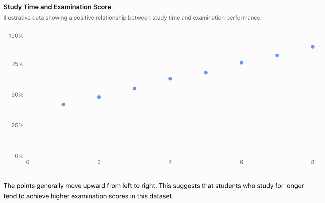
The points generally move upward from left to right. This suggests that students who study for longer tend to achieve higher examination scores in this dataset.
This is an example of positive correlation.
Notice that the graph shows an association. It does not establish that additional study time alone caused the higher scores.
Constructing a Scatter Plot
To construct a scatter plot correctly, follow these steps.
-
Identify the variables. Decide which variable belongs on each axis.
-
Choose suitable scales. Make sure the scales include all the observations and use consistent intervals.
-
Label both axes. Include the variable names and units where appropriate.
-
Plot each coordinate pair. For example, (3, 55) represents 3 hours of study and a score of 55%.
-
Examine the pattern. Look for direction, strength, shape, clusters, and unusual points.
Unlike a line graph showing measurements over time, a scatter plot generally does not connect consecutive points.
Worked Example: Constructing a Scatter Plot
A scientist records the temperature and number of ice creams sold at a shop.
|
Temperature (°C) |
Ice creams sold |
|---|---|
|
20 |
30 |
|
22 |
42 |
|
24 |
50 |
|
26 |
65 |
|
28 |
73 |
|
30 |
88 |
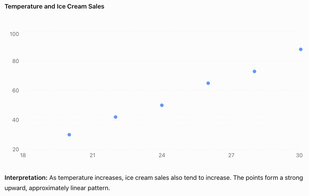
Understanding Correlation
Correlation describes the direction and strength of an association between two variables.
For linear relationships, there are three main directions.
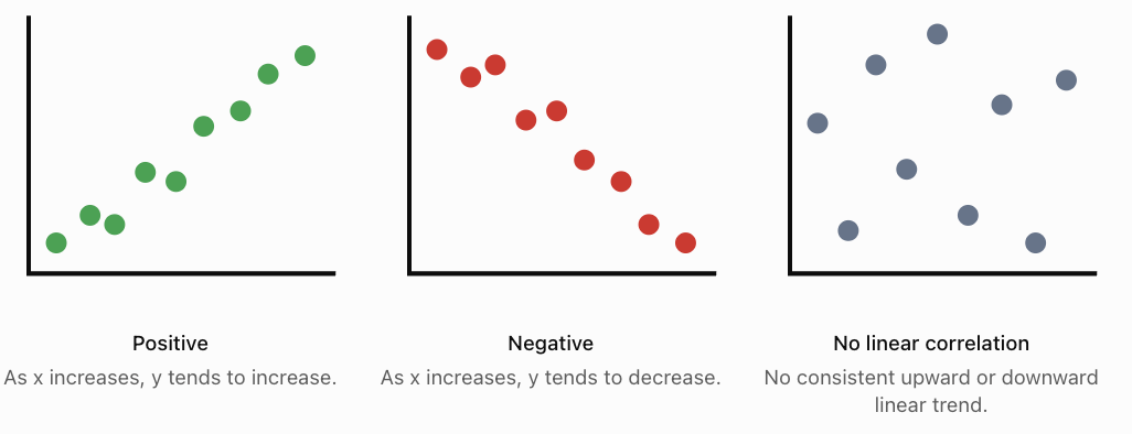
Positive Correlation
Positive correlation occurs when larger values of one variable tend to be associated with larger values of another.
Examples include height and arm span, temperature and ice cream sales, and hours of exercise and calories burned during exercise.
Negative Correlation
Negative correlation occurs when larger values of one variable tend to be associated with smaller values of another.
Examples include vehicle age and resale value, distance remaining and distance travelled along a fixed route, and time spent braking and vehicle speed during a braking event.
No Linear Correlation
Two variables have little or no linear correlation when there is no consistent straight-line trend.
For example, a dataset comparing students' shoe sizes and examination scores might show no meaningful linear association.
Importantly, no linear correlation does not necessarily mean there is no relationship at all. The relationship might be curved.
Strength of Correlation
The strength of linear correlation describes how closely the points follow a straight-line pattern.
-
Strong correlation: Points lie close to a straight line.
-
Moderate correlation: A general trend is visible, but points are more spread out.
-
Weak correlation: Points are widely scattered, with only a slight linear trend.
-
Perfect correlation: Every point lies exactly on a straight line.
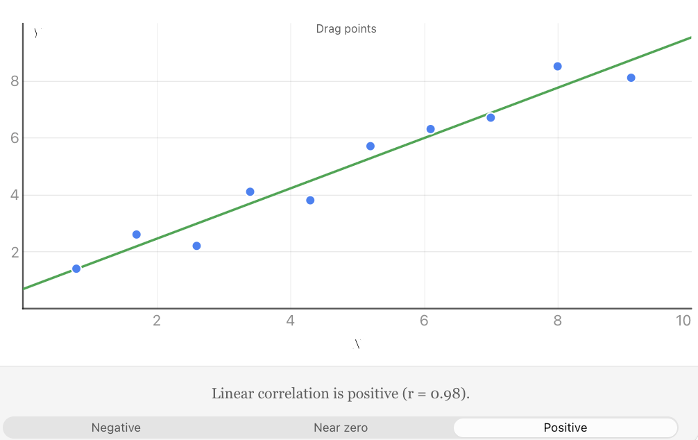
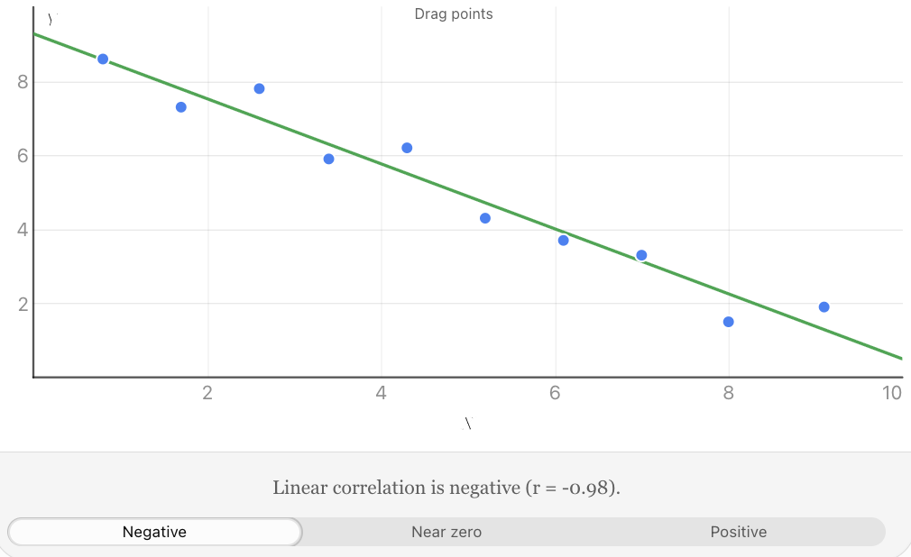
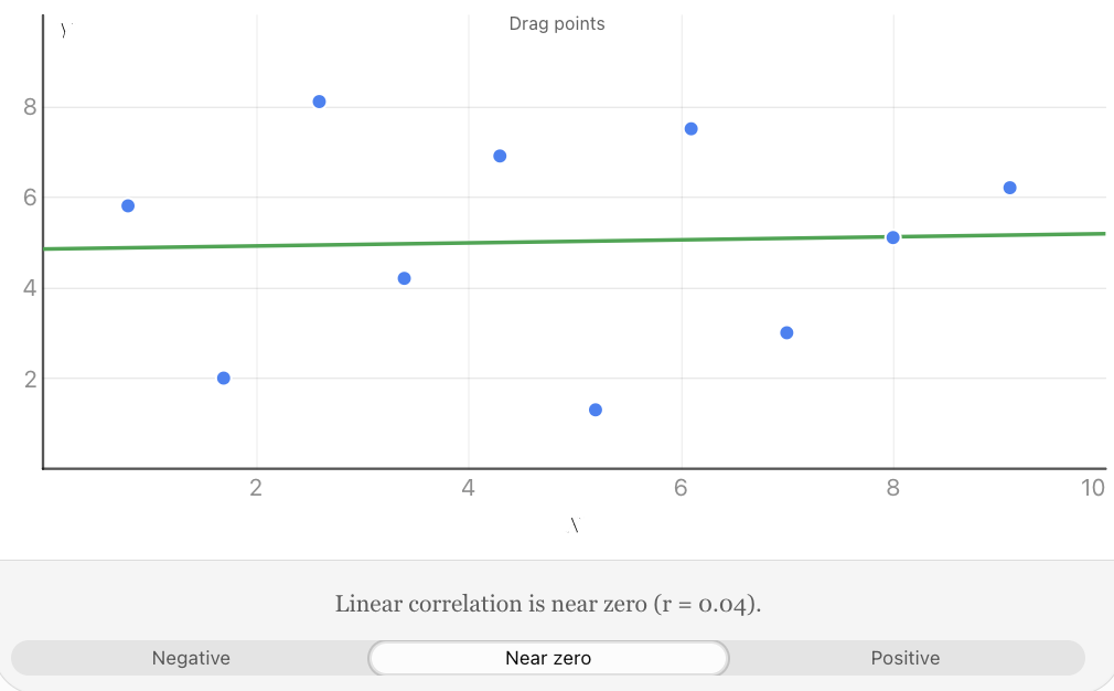
Explore the positive, negative, and uncorrelated patterns. Move individual points and observe how the correlation coefficient changes.
The strength of a relationship is different from its direction. A strong negative correlation can be just as strong as a strong positive correlation.
The Pearson Correlation Coefficient
Visual inspection of a scatter plot is useful, but statisticians often need a numerical measurement.
The Pearson correlation coefficient, represented by r, measures the strength and direction of a linear relationship between two quantitative variables.
Its value is always between −1 and +1.
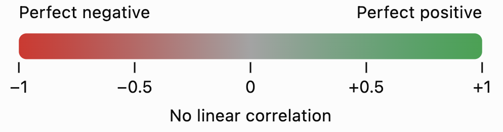
The main interpretations are:
Value of r
Interpretation
+1
Perfect positive linear correlation
+0.8
Strong positive linear correlation
+0.4
Moderate positive linear correlation
0
No linear correlation
−0.4
Moderate negative linear correlation
−0.8
Strong negative linear correlation
−1
Perfect negative linear correlation
These descriptions are approximate. There is no universally accepted boundary between weak, moderate, and strong correlation; interpretations depend on the field and context.
Calculating Pearson's r
The computational formula is:
\[ r=\frac{n\sum xy-(\sum x)(\sum y)} {\sqrt{[n\sum x^2-(\sum x)^2][n\sum y^2-(\sum y)^2]}} \]Where:
-
n = number of paired observations
-
Σx = sum of all x-values
-
Σy = sum of all y-values
-
Σxy = sum of the products of paired values
-
Σx² = sum of the squared x-values
-
Σy² = sum of the squared y-values
The symbol Σ means "sum of."
This formula is suitable when both variables vary and the observations are paired.
Worked Example: Calculating a Correlation Coefficient
Five students complete a practice exercise. Their study time and scores are recorded.
x (hours)
y (score)
x²
y²
xy
1
2
1
4
2
2
3
4
9
6
3
5
9
25
15
4
4
16
16
16
5
6
25
36
30
15
20
55
90
69
Step 1: Identify the totals.
n = 5
Σx = 15
Σy = 20
Σx² = 55
Σy² = 90
Σxy = 69
Step 2: Substitute into the formula.
\[ r=\frac{5(69)-(15)(20)} {\sqrt{[5(55)-15^2][5(90)-20^2]}} \]Step 3: Simplify.
\[ r=\frac{345-300}{\sqrt{(275-225)(450-400)}} \]\[ r=\frac{45}{\sqrt{2500}}=\frac{45}{50} \]\[ \boxed{r=0.90} \]Interpretation: There is a strong positive linear correlation between study time and exercise score in this small dataset.
Students who studied for longer generally achieved higher scores, although the relationship was not perfect.
Calculating Correlation Using Technology
For larger datasets, calculations are usually completed using a spreadsheet, graphing calculator, or statistical software.
In Excel or Google Sheets, if the x-values are in cells A2:A11 and y-values are in B2:B11, enter:
=CORREL(A2:A11,B2:B11)The spreadsheet calculates Pearson's r automatically.
The correlation coefficient measures association; it does not indicate which variable causes the other.
Interpreting Relationships Between Variables
A scatter plot provides more information than simply whether a correlation is positive or negative.
When analysing a scatter plot, consider five important features.
Direction
Does the relationship increase, decrease, or show no consistent linear trend?
Strength
How closely do the points follow the overall pattern?
Form
Is the relationship approximately linear or nonlinear?
A linear relationship follows an approximately straight-line pattern. A nonlinear relationship may follow a curve.
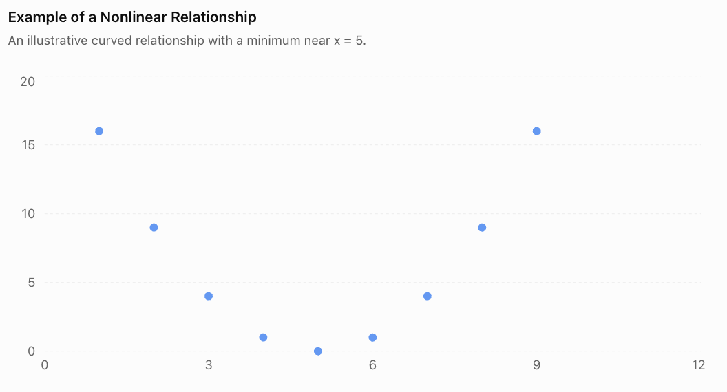
The points form a U-shaped pattern. There is a clear relationship, even though the Pearson correlation coefficient is zero for this symmetric dataset.
This demonstrates why we should inspect the scatter plot before relying on r.
Outliers
An outlier is a point that lies unusually far from the overall pattern.
An outlier may result from measurement error, incorrect data entry, an unusual event, or genuine variation.
Outliers can substantially affect Pearson's correlation coefficient.
Clusters and Subgroups
Sometimes a scatter plot contains separate groups of points.
For example, data from two different age groups might form two clusters. A correlation calculated using all the data may hide important differences within the groups.
When possible, examine the relationship within relevant subgroups as well as across the full dataset.
Lines of Best Fit
A line of best fit, or regression line, summarises an approximately linear relationship between two variables.
It can be used to estimate the value of y for a given x.
A linear model is commonly written as:
\[ y=mx+b \]Where:
-
m = slope of the line
-
b = y-intercept
The slope indicates the predicted change in y for each one-unit increase in x.
Worked Example: Predicting Examination Scores
Suppose a regression model relating study time to examination score is:
\[ y=7x+35 \]Where x represents study time in hours and y represents predicted examination score.
Predict the score for a student who studies for 6 hours.
Substitute x = 6:
\[ y=7(6)+35 \]\[ y=42+35=\boxed{77} \]The predicted score is 77%.
This is a model-based prediction, not a guarantee.
Interpolation and Extrapolation
Interpolation means predicting within the range of observed data.
Extrapolation means predicting beyond the observed range.
For example, if study times were measured from 1 to 8 hours:
-
Predicting the score for 6 hours is interpolation.
-
Predicting the score for 20 hours is extrapolation.
Extrapolation is generally less reliable because the relationship may change outside the observed range. A linear examination-score model, for example, cannot reasonably predict scores above 100%.
Correlation Does Not Imply Causation
One of the most important principles in statistics is that a relationship between two variables does not automatically mean that one variable causes the other.
Correlation means two variables are statistically associated.
Causation means a change in one variable produces a change in another.
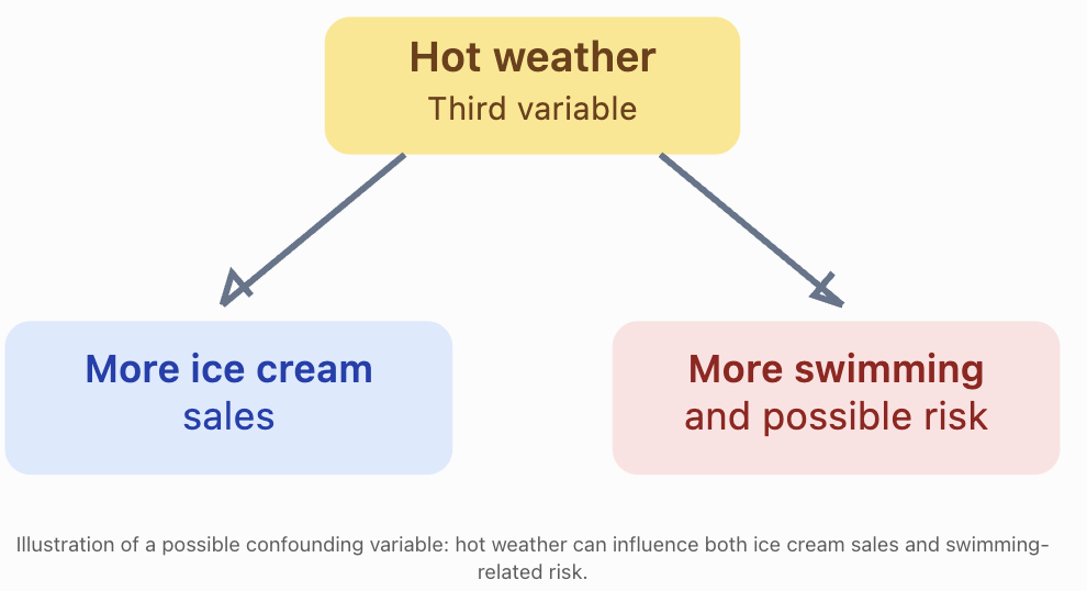
Example: Ice Cream Sales and Drowning Incidents
During hotter weather, both ice cream sales and swimming activity may increase. Drowning incidents may also increase when more people are swimming.
A statistical study might find a positive correlation between ice cream sales and drowning incidents.
Does buying ice cream cause drowning?
No.
A third variable, such as hot weather, may help explain the association.
Other Reasons Correlation May Not Establish Causation
Reverse causation: The proposed direction of cause and effect may be incorrect. For example, a relationship between anxiety and poor sleep could involve effects in both directions.
Confounding variables: A third factor may influence both variables.
Coincidence: Two variables may be correlated by chance, particularly when many comparisons are tested.
Selection bias: The way participants or observations are selected may produce a misleading relationship.
How Can Causation Be Investigated?
Researchers can strengthen causal conclusions by using:
-
Randomised controlled experiments, where appropriate and ethical.
-
Longitudinal studies that examine how variables change over time.
-
Careful measurement and control of confounding variables.
-
Replication of findings in different populations.
-
Plausible scientific explanations supported by additional evidence.
Even a very high correlation coefficient, such as r = 0.99, is not by itself proof of causation.
Real-World Applications
Meteorology
Scientists investigate relationships between temperature, humidity, rainfall, and atmospheric pressure. Scatter plots can help identify patterns and evaluate weather models.
Sports Science
Researchers compare exercise intensity with heart rate, oxygen consumption, and recovery time to understand athletic performance.
Economics and Property
Analysts examine associations between property size, location, age, and selling price. Regression models can support price estimates.
Environmental Science
Scientists investigate relationships between pollution levels, water temperature, and aquatic biodiversity. Correlations can help identify environmental questions requiring further investigation.
Common Mistakes
Common mistake
Correction
Assuming positive correlation means a strong relationship
Positive describes direction, not strength.
Thinking r = −0.9 is weaker than r = +0.5
The absolute value of r determines linear strength; 0.9 is stronger than 0.5.
Assuming r = 0 means there is no relationship
There may be a nonlinear relationship.
Connecting every point in a scatter plot
Generally plot the points separately and examine the overall pattern.
Claiming that correlation proves causation
Consider confounding variables, reverse causation, and other explanations.
Ignoring unusual points
Outliers can greatly change the correlation coefficient.
Making predictions far beyond observed values
Extrapolation may produce unrealistic predictions.
Calculating r from unpaired or incorrectly matched observations
Each x-value must be matched with its corresponding y-value.
Key Terms
-
Scatter plot: A graph showing pairs of numerical observations as points.
-
Bivariate data: Data involving two variables measured together.
-
Explanatory variable: A variable used to help explain or predict another variable.
-
Response variable: The variable being investigated or predicted.
-
Correlation: A statistical association between variables.
-
Positive correlation: An association in which larger values of one variable tend to accompany larger values of another.
-
Negative correlation: An association in which larger values of one variable tend to accompany smaller values of another.
-
Linear correlation: An association described by an approximately straight-line pattern.
-
Pearson correlation coefficient (r): A numerical measure of the direction and strength of a linear relationship.
-
Outlier: An observation that lies unusually far from the overall pattern.
-
Line of best fit: A line used to summarise and predict an approximately linear relationship.
-
Regression: A statistical method for modelling relationships between variables.
-
Interpolation: Prediction within the observed data range.
-
Extrapolation: Prediction outside the observed data range.
-
Causation: A relationship in which one factor produces a change in another.
-
Confounding variable: A variable that can distort the apparent relationship between the variables being studied.
Key Takeaways
-
Scatter plots display paired quantitative data and help reveal relationships between two variables.
-
Correlation can be positive, negative, or show little or no linear association.
-
Correlation strength depends on how closely the points follow a linear pattern.
-
Pearson's correlation coefficient, r, ranges from −1 to +1.
-
Values of r close to −1 or +1 indicate strong linear correlation; values near zero indicate weak linear correlation.
-
A scatter plot should be inspected for outliers, clusters, and nonlinear patterns before interpreting r.
-
Regression lines can be used to make predictions, but predictions outside the observed range require caution.
-
Correlation alone cannot establish a cause-and-effect relationship.
Check Your Understanding
Question 1: Identifying Correlation
A dataset shows that as the age of a car increases, its resale value generally decreases.
What type of correlation does this represent?
Question 2: Interpreting Strength
Three datasets have correlation coefficients:
-
Dataset A: r = 0.92
-
Dataset B: r = −0.75
-
Dataset C: r = 0.18
Which dataset has the strongest linear correlation? Which has the weakest?
Question 3: Constructing a Scatter Plot
The table shows the number of hours students spend exercising each week and their resting heart rates.
Exercise (hours)
Resting heart rate (bpm)
1
82
2
79
3
75
4
73
5
69
6
66
Construct a scatter plot, identify the correlation direction, and describe its strength.
Question 4: Calculating Pearson's r
Calculate the Pearson correlation coefficient for the following dataset.
x
y
1
3
2
5
3
4
4
7
Interpret your result.
Question 5: Correlation and Causation
A researcher discovers that cities with more firefighters tend to experience greater total property damage from fires.
A newspaper concludes that employing more firefighters causes greater property damage.
Explain why this conclusion is not justified.
Question 6: Evaluating a Statistical Relationship
A scatter plot of x and y shows a clear U-shaped pattern.
The Pearson correlation coefficient is r = 0.02.
A student concludes that x and y are unrelated.
Explain the problem with this conclusion.
Question 7: Making Predictions
A regression model predicts electricity consumption using:
y = 12x + 150
Where x is the average daily temperature in °C and y is daily electricity consumption in kWh.
Calculate the predicted electricity consumption at 25°C.
Explain why using this model to predict consumption at 70°C might be unreliable if the observed temperatures ranged from 15°C to 35°C.
Fully Worked Answers
Answer 1
The relationship is a negative correlation.
As car age increases, resale value generally decreases.
Answer 2
Compare the absolute values:
Dataset
r
Absolute value
A
0.92
0.92
B
−0.75
0.75
C
0.18
0.18
Dataset A has the strongest linear correlation.
Dataset C has the weakest linear correlation.
The negative sign for Dataset B describes direction, not weakness.
Answer 3
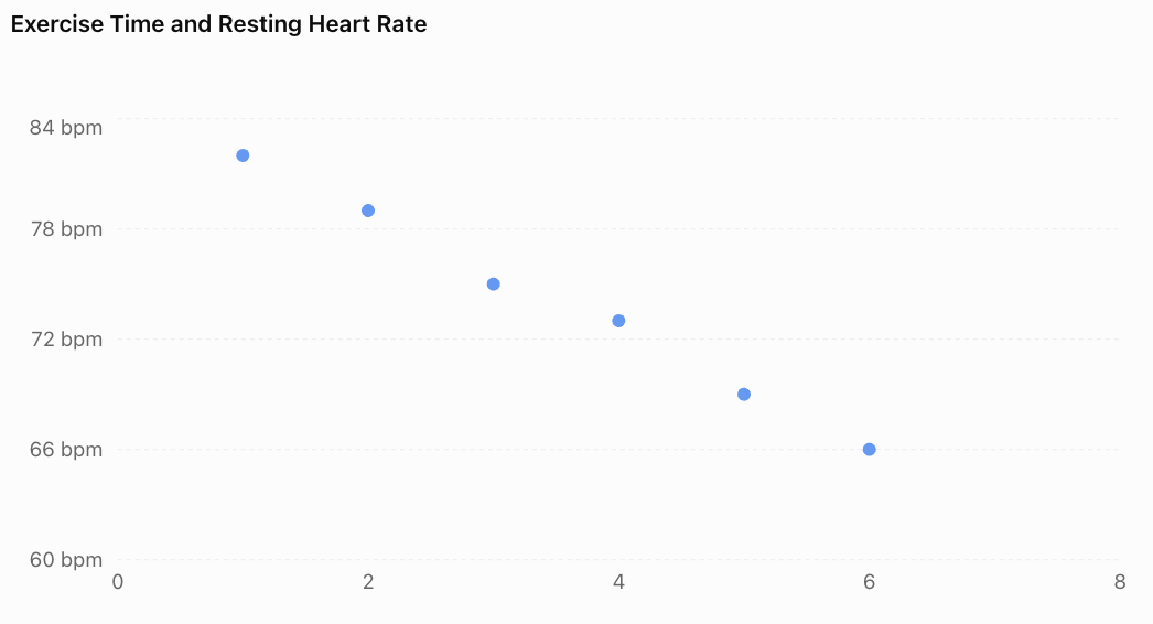
The graph shows a strong negative linear correlation.
As weekly exercise time increases, resting heart rate tends to decrease in this dataset.
This does not establish that exercise time alone caused the differences in resting heart rate.
Answer 4
First calculate the required totals.
x
y
x²
y²
xy
1
3
1
9
3
2
5
4
25
10
3
4
9
16
12
4
7
16
49
28
10
16
30
99
53
n = 4
Substitute:
\[ r=\frac{4(53)-(10)(16)} {\sqrt{[4(30)-10^2][4(99)-16^2]}} \]\[ r=\frac{212-160}{\sqrt{(120-100)(396-256)}} \]\[ r=\frac{52}{\sqrt{2800}} \]\[ \boxed{r\approx0.983} \]The result indicates a very strong positive linear correlation.
Answer 5
Cities with more firefighters may be larger or experience more fires, including more serious fires.
These factors could explain why they also experience greater total property damage.
The correlation does not demonstrate that firefighters cause damage.
A better investigation would consider city size, number of fires, fire severity, building density, and other relevant variables.
Answer 6
Pearson's r measures linear correlation.
A U-shaped relationship is nonlinear. Therefore, r can be close to zero even when the variables have a clear mathematical relationship.
The student should examine the scatter plot and consider a nonlinear model rather than concluding that the variables are unrelated.
Answer 7
Given:
y = 12x + 150
Substitute x = 25:
y = 12(25) + 150
y = 300 + 150
Predicted electricity consumption = 450 kWh.
Predicting at 70°C would be extrapolation because 70°C lies far outside the observed range of 15°C to 35°C.
The original linear relationship may not continue at extreme temperatures, making the prediction unreliable.
Final Reflection
Scatter plots and correlation provide powerful tools for exploring relationships in data. They help us identify patterns, describe the strength and direction of associations, and make informed predictions.
However, responsible statistical reasoning requires more than calculating a correlation coefficient. We must examine the shape of the data, recognise unusual observations, evaluate the reliability of predictions, and consider alternative explanations.
The most important distinction is that a statistical relationship is evidence of association, not automatic proof of cause and effect.
-
2. Linear Regression
Learning outcomes
- I can determine a line of best fit.
- I can interpret regression equations.
- I can make predictions using regression.
- I can analyse residuals.
- I can evaluate model accuracy.
Introduction
Imagine that a school wants to investigate whether the number of hours students spend studying can help predict their examination scores. After collecting data, the school notices that students who study longer generally achieve higher scores. However, the points on a scatter plot do not form a perfectly straight line.
How can we describe this relationship mathematically? How can we use it to predict examination results? And how can we determine whether our predictions are reliable?
Linear regression provides a method for answering these questions.
Linear regression is a statistical technique that models the relationship between a numerical explanatory variable and a numerical response variable using a straight line. It allows us to identify trends, make predictions, measure prediction errors, and evaluate how well a mathematical model represents real data.
Linear regression is widely used in science, economics, engineering, medicine, environmental research, and business.
What Is Linear Regression?
Linear regression is a method of finding a straight line that best describes the relationship between two quantitative variables.
This line is called the regression line, or line of best fit.
A scatter plot displays the original observations, while the regression line summarises their overall linear trend.
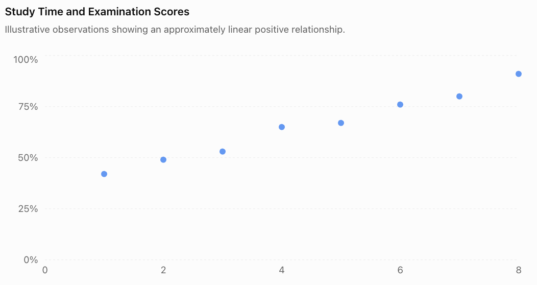
The points generally rise from left to right, indicating a positive linear association.
A regression line allows us to represent this trend with an equation rather than simply describing it visually.
The Regression Equation
A simple linear regression equation is commonly written as:
Where:
-
ŷ (y-hat) = predicted value of the response variable
-
x = explanatory or predictor variable
-
a = y-intercept of the regression line
-
b = slope or regression coefficient
The symbol ŷ is used instead of y because the regression equation produces a prediction, which may differ from the observed value.
Understanding the Slope
The slope, b, describes how much the predicted response changes for each one-unit increase in x.
-
If b is positive, the predicted response increases as x increases.
-
If b is negative, the predicted response decreases as x increases.
-
If b is zero, the model predicts the same response regardless of x.
Understanding the Intercept
The intercept, a, is the predicted response when x = 0.
However, the intercept is not always meaningful in a real-world context. If zero lies outside the observed range, interpreting the intercept may involve unreliable extrapolation.
Determining a Line of Best Fit
A line of best fit can be estimated visually or calculated mathematically.
Method 1: Drawing a Line of Best Fit by Eye
When using a scatter plot:
-
Plot all paired observations accurately.
-
Identify the overall direction of the points.
-
Draw a straight line through the centre of the pattern.
-
Try to balance the points above and below the line.
-
Choose two well-separated points on the line to estimate its slope and intercept.
A visually estimated line is useful for understanding trends, but different people may draw slightly different lines.
For precise statistical analysis, we use the least-squares method.
Method 2: The Least-Squares Regression Line
The least-squares method finds the line that minimises the sum of the squared vertical differences between observed and predicted values.
These vertical differences are called residuals.
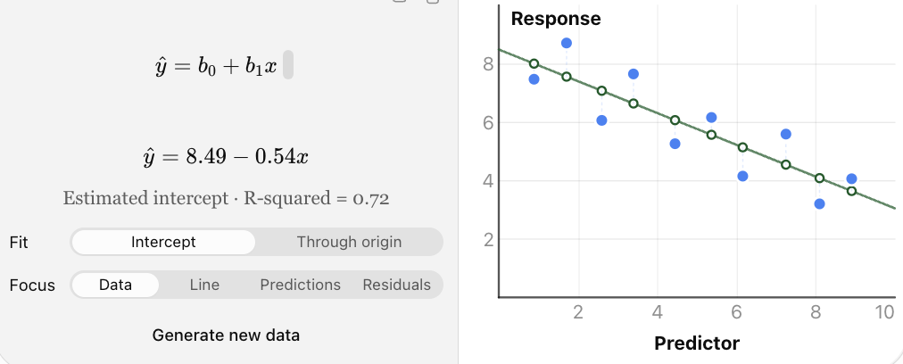
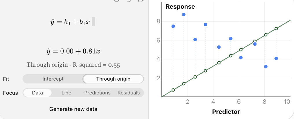
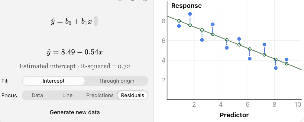
Interactive regression model: move the observed points to see how the least-squares line changes. The vertical gaps between points and the fitted line represent residuals.
Why square the residuals?
Squaring ensures that positive and negative errors do not cancel each other. It also gives greater weight to large errors.
The quantity minimised is called the sum of squared errors, or SSE:
The least-squares line has the smallest possible SSE among straight lines with an intercept fitted to the same dataset.
Calculating the Least-Squares Regression Line
For simple linear regression, the slope is:
The intercept is:
Where:
-
n = number of paired observations
-
Σxy = sum of products of corresponding x- and y-values
-
Σx = sum of x-values
-
Σy = sum of y-values
-
Σx² = sum of squared x-values
-
x̄ = mean of x-values
-
ȳ = mean of y-values
The slope formula requires variation in x; if all x-values are identical, the usual least-squares slope cannot be calculated.
Worked Example 1: Finding a Regression Equation
A teacher records the number of hours five students spend studying and their scores on a short assessment.
|
Study time, x |
Score, y |
|---|---|
|
1 |
2 |
|
2 |
3 |
|
3 |
5 |
|
4 |
4 |
|
5 |
6 |
Determine the least-squares regression equation.
Step 1: Construct a calculation table.
|
x |
y |
x² |
xy |
|---|---|---|---|
|
1 |
2 |
1 |
2 |
|
2 |
3 |
4 |
6 |
|
3 |
5 |
9 |
15 |
|
4 |
4 |
16 |
16 |
|
5 |
6 |
25 |
30 |
|
15 |
20 |
55 |
69 |
Therefore:
n = 5
Σx = 15
Σy = 20
Σx² = 55
Σxy = 69
Step 2: Calculate the slope.
Step 3: Calculate the means.
Step 4: Calculate the intercept.
Step 5: Write the regression equation.
This equation represents the least-squares line of best fit.
Interpreting the Equation
The slope of 0.9 means that each additional hour of study is associated with an increase of 0.9 points in the predicted assessment score.
The intercept of 1.3 means that the model predicts a score of 1.3 points when study time is zero hours.
Because zero hours is outside the observed study-time range of 1–5 hours, the intercept should be interpreted cautiously.
Making Predictions Using Regression
Once a regression equation has been determined, it can be used to estimate the response variable for a particular explanatory-variable value.
Worked Example 2: Predicting an Assessment Score
Using the regression equation:
ŷ = 1.3 + 0.9x
Predict the assessment score for a student who studies for 4 hours.
Step 1: Substitute x = 4.
ŷ = 1.3 + 0.9(4)
Step 2: Simplify.
ŷ = 1.3 + 3.6
The predicted score is 4.9 points.
The actual score of the student who studied for 4 hours was 4 points, illustrating that a regression prediction does not necessarily match an observation exactly.
Worked Example 3: Predicting House Prices
Suppose a property analyst develops the model:
ŷ = 80,000 + 2,500x
Where:
-
x = floor area in square metres
-
ŷ = predicted house price in dollars
Predict the price of a house with a floor area of 120 m².
ŷ = 80,000 + 2,500(120)
ŷ = 80,000 + 300,000
The model predicts a price of $380,000.
The slope indicates an additional $2,500 in predicted price per square metre of floor area.
This does not mean that increasing a particular house's area by one square metre would necessarily cause its price to rise by exactly $2,500. Other factors, such as location and condition, also matter.
Interpolation and Extrapolation
Regression predictions are not equally reliable for all values of x.
Interpolation
Interpolation occurs when a prediction is made within the range of x-values used to develop the model.
For example, if study times range from 1 to 8 hours, predicting a score for 5 hours is interpolation.
Extrapolation
Extrapolation occurs when a prediction is made outside the observed range.
Predicting the score for a student who studies for 20 hours would be extrapolation.
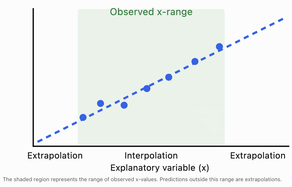
Extrapolation is often less reliable because the relationship may change outside the observed range.
For example, a model relating study time to examination score cannot reasonably predict examination scores greater than 100% indefinitely.
Understanding Residuals
A regression line does not usually pass through every observation.
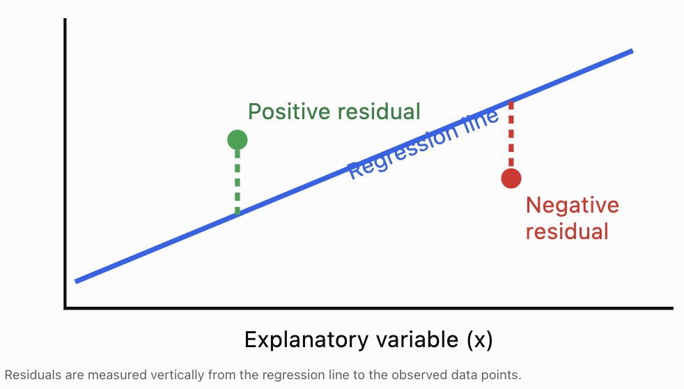
The difference between an observed value and its predicted value is called a residual.
The residual formula is:
Where:
-
e = residual
-
y = observed value
-
ŷ = predicted value
A residual measures the prediction error for one observation.
Interpreting Residual Signs
-
Positive residual: The observed value is greater than predicted; the point lies above the regression line.
-
Negative residual: The observed value is less than predicted; the point lies below the regression line.
-
Zero residual: The observed value equals the predicted value; the point lies on the regression line.
Worked Example 4: Calculating Residuals
Use the regression equation from Worked Example 1:
ŷ = 1.3 + 0.9x
Calculate the predicted values and residuals for all five students.
x
Observed y
Predicted ŷ
Residual (y − ŷ)
1
2
2.2
−0.2
2
3
3.1
−0.1
3
5
4.0
+1.0
4
4
4.9
−0.9
5
6
5.8
+0.2
For the third student:
e = 5 − 4.0 = +1.0
The actual score was 1 point higher than predicted.
For the fourth student:
e = 4 − 4.9 = −0.9
The actual score was 0.9 points lower than predicted.
For an ordinary least-squares regression with an intercept, the residuals sum to zero, apart from rounding.
Here:
−0.2 − 0.1 + 1.0 − 0.9 + 0.2 = 0
This property does not mean the predictions are perfect; positive and negative residuals can cancel.
Residual Plots
A residual plot displays residuals on the vertical axis and the explanatory variable (or fitted values) on the horizontal axis.
Residual plots are useful for checking whether a linear model is appropriate.
For the five-student example:
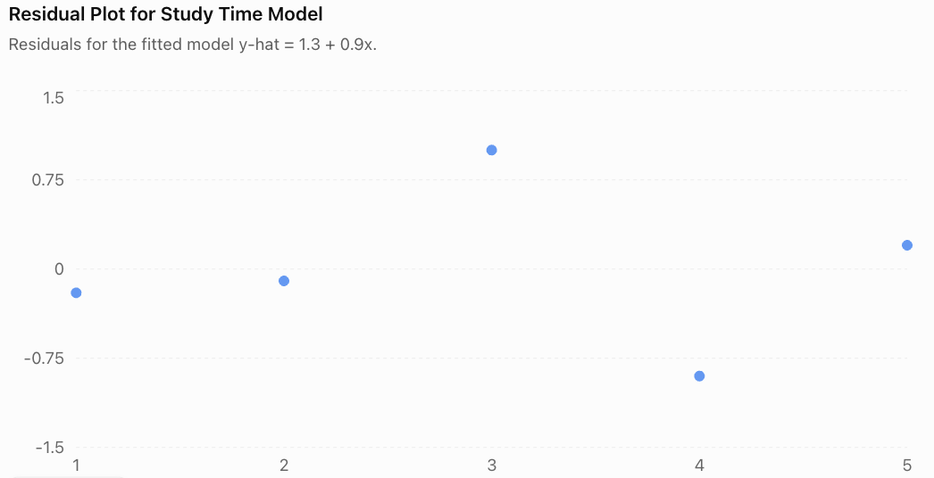
The residuals appear on both sides of zero without a clear curved trend. This is consistent with a linear model, although five observations are too few to assess model assumptions confidently.
Recognising Residual Patterns
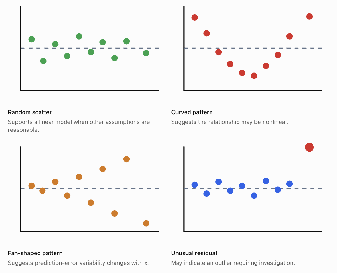
A good residual plot should generally show points scattered around zero without an obvious systematic pattern.
A curved pattern suggests that a straight line may not adequately describe the relationship.
A fan-shaped pattern suggests heteroscedasticity, meaning that the variability of errors changes across the predictor range.
Residual plots can also help identify unusual observations, although additional diagnostics may be needed.
Evaluating Model Accuracy
Finding a regression equation is only the beginning. We must also determine how accurately the model describes the data and how useful its predictions are.
Several statistical measures help us evaluate model performance.
Sum of Squared Errors (SSE)
SSE measures the total squared prediction error:
\[ SSE=\sum (y-\hat y)^2 \]Smaller SSE values indicate a closer fit for models evaluated on the same observations and response scale.
Using the five-student dataset:
Residual
Residual²
−0.2
0.04
−0.1
0.01
+1.0
1.00
−0.9
0.81
+0.2
0.04
Total
1.90
Therefore:
\[ \boxed{SSE=1.90} \]Mean Squared Error (MSE)
MSE is the average squared prediction error.
For descriptive or predictive evaluation of n observations:
\[ MSE=\frac{SSE}{n} \]For our dataset:
\[ MSE=\frac{1.90}{5}=\boxed{0.38} \]Smaller MSE values generally indicate better predictions on comparable data.
In statistical inference, a related estimate of residual error variance uses SSE/(n − 2) for simple linear regression with an intercept. This accounts for the two fitted parameters.
Root Mean Squared Error (RMSE)
RMSE is the square root of MSE.
\[ RMSE=\sqrt{\frac{SSE}{n}} \]For the five-student dataset:
\[ RMSE=\sqrt{0.38} \]\[ \boxed{RMSE\approx0.616} \]The RMSE is approximately 0.616 assessment points.
Unlike MSE, RMSE is expressed in the same units as the response variable, making it easier to interpret.
Mean Absolute Error (MAE)
MAE measures the average absolute prediction error.
\[ MAE=\frac{\sum |y-\hat y|}{n} \]For our dataset:
\[ MAE=\frac{0.2+0.1+1.0+0.9+0.2}{5} \]\[ MAE=\frac{2.4}{5}=\boxed{0.48} \]The average absolute prediction error is 0.48 points.
Unlike MSE and RMSE, MAE does not square errors, so it is less sensitive to a small number of very large errors.
The Coefficient of Determination: R²
The coefficient of determination, written R², describes the proportion of variation in the response variable explained by the fitted regression model relative to a model that always predicts the sample mean.
For ordinary least-squares regression with an intercept:
\[ R^2=1-\frac{SSE}{SST} \]Where:
-
SSE = sum of squared residuals
-
SST = total sum of squares
-
SST = Σ(y − ȳ)²
For simple linear regression with an intercept, R² is also equal to the square of the Pearson correlation coefficient.
\[ R^2=r^2 \]Worked Example 5: Calculating R²
For our five-student dataset:
y-values: 2, 3, 5, 4, 6
Mean score:
ȳ = 4
Calculate SST:
SST = (2 − 4)² + (3 − 4)² + (5 − 4)² + (4 − 4)² + (6 − 4)²
SST = 4 + 1 + 1 + 0 + 4
SST = 10
We previously calculated SSE = 1.90.
Therefore:
\[ R^2=1-\frac{1.90}{10} \]\[ \boxed{R^2=0.81} \]The model accounts for 81% of the variation in assessment scores within this dataset, relative to predicting the mean score.
The remaining 19% is not explained by the fitted line.
This does not mean that study time causes exactly 81% of examination performance. R² measures model fit, not causation.

Interpreting R² Carefully
A high R² indicates that the fitted model explains a large proportion of the observed variation.
However, a high R² does not guarantee that:
-
The relationship is causal.
-
The model is appropriate for every situation.
-
The model will predict new observations accurately.
-
There are no influential outliers.
-
The model's assumptions are satisfied.
Similarly, a low R² does not automatically make a model useless. In fields involving highly variable human behaviour, even modest predictive relationships may be informative.
Comparing Measures of Model Accuracy
Measure
What it measures
Preferred direction
SSE
Total squared residual error
Lower
MSE
Average squared prediction error
Lower
RMSE
Typical error scale, with large errors emphasised
Lower
MAE
Average absolute prediction error
Lower
R²
Proportion of sample variation explained by the model
Higher
These measures should be compared only when appropriate. For example, SSE depends on the number of observations, while MSE and RMSE depend on the scale of the response variable.
A model should also be tested on data that were not used to fit it.
Training Data and Test Data
A regression model may fit the observations used to construct it very well but perform poorly on new data.
This is called overfitting when the model captures patterns or noise that do not generalise.
To evaluate predictive performance, statisticians often divide data into:
-
Training data: Used to calculate the regression equation.
-
Test data: Used to evaluate predictions on observations not used to fit the model.
For smaller datasets, cross-validation may provide a more informative assessment than a single train–test split.
Worked Example 6: Comparing Two Models
Two regression models are evaluated on the same unseen test dataset.
Measure
Model A
Model B
Training RMSE
2.1
1.2
Test RMSE
2.4
5.8
Training R²
0.88
0.97
Model B fits the training data more closely, but Model A makes substantially smaller errors on the test data.
Therefore, Model A is the better predictive choice based on these test results.
Model B may have overfitted the training observations.
This example illustrates why model evaluation should not rely only on training accuracy.
Assumptions of Linear Regression
Linear regression is most reliable when its underlying assumptions are reasonably satisfied.
Linearity
The mean response should have an approximately linear relationship with the explanatory variable.
A curved residual pattern suggests that a linear model may be inappropriate.
Independence
Observations or model errors should be independent where required by the study design.
For example, measurements collected repeatedly from the same person may be related and require specialised methods.
Constant Error Variance
The spread of errors should remain approximately constant across fitted values for standard regression inference.
A fan-shaped residual plot may indicate that this assumption is violated.
Approximately Normal Errors for Certain Inference Procedures
Normality of errors is particularly relevant for exact small-sample confidence intervals and hypothesis tests.
Normality is not required simply to calculate the least-squares line.
Absence of Highly Influential Observations
An extreme observation can substantially change the slope and intercept.
Researchers should investigate unusual observations rather than automatically deleting them.
Other Important Considerations
Even if these assumptions are reasonably satisfied, omitted variables, measurement errors, biased sampling, or inappropriate extrapolation can limit a model's usefulness.
Using Technology for Linear Regression
Regression calculations can be performed using spreadsheets, graphing calculators, and statistical software.
In Excel or Google Sheets, suppose the x-values are in A2:A11 and y-values are in B2:B11.
Purpose
Formula
Calculate slope
=SLOPE(B2:B11,A2:A11)Calculate intercept
=INTERCEPT(B2:B11,A2:A11)Calculate R²
=RSQ(B2:B11,A2:A11)Calculate Pearson's r
=CORREL(A2:A11,B2:B11)To make a prediction, use:
=INTERCEPT(B2:B11,A2:A11)+SLOPE(B2:B11,A2:A11)*D2Where D2 contains the x-value for which a prediction is required.
For a visual approach, create a scatter plot and add a linear trendline, selecting the options to display the equation and R² value.
Remember that spreadsheet software may round the displayed equation. Calculations using full-precision coefficients are generally more accurate.
Real-World Applications of Linear Regression
Climate and Environmental Science
Researchers use regression to investigate temperature trends, rainfall patterns, pollution concentrations, and environmental changes over time.
Engineering
Engineers model relationships between applied force and deformation, electrical current and voltage, or material properties and performance.
Business and Economics
Analysts use regression to predict sales, examine relationships between advertising and revenue, and estimate how prices vary with product characteristics.
Medicine and Health Research
Researchers investigate relationships between age, physical measurements, exercise, and health outcomes. Regression helps quantify associations while accounting for uncertainty.
Common Mistakes
Common mistake
Correction
Assuming a regression line passes through every observation
The line minimises total squared residuals; individual residuals are usually nonzero.
Confusing observed y with predicted ŷ
Use y for actual measurements and ŷ for predictions.
Calculating residuals as ŷ − y
Residual = observed − predicted.
Interpreting the intercept without considering context
The intercept may be meaningless if x = 0 is outside the observed range.
Assuming a high R² proves causation
R² describes model fit, not cause and effect.
Ignoring residual patterns
Curved or fan-shaped patterns can reveal model problems.
Extrapolating far beyond the data
The relationship may change outside the observed range.
Comparing SSE values from different-sized datasets without caution
SSE depends on sample size and response scale.
Assuming low training error guarantees accurate predictions
Evaluate the model on unseen data.
Automatically removing outliers
Investigate unusual observations and their influence before deciding how to handle them.
Key Terms
-
Linear regression: A statistical method that models a relationship between numerical variables using a straight line.
-
Regression line: A fitted line used to summarise a linear relationship and make predictions.
-
Line of best fit: A line that represents the overall trend in a scatter plot.
-
Least-squares method: A method that minimises the sum of squared residuals.
-
Explanatory variable: A variable used to predict or explain another variable.
-
Response variable: The variable being predicted or studied.
-
Predicted value (ŷ): The response value calculated using the regression equation.
-
Regression coefficient: A parameter of a regression model, such as its slope.
-
Slope: The predicted change in y for a one-unit increase in x.
-
Intercept: The predicted y-value when x = 0.
-
Residual: The difference between an observed and predicted value.
-
Residual plot: A graph used to investigate patterns in regression errors.
-
SSE: Sum of squared errors.
-
MSE: Mean squared error.
-
RMSE: Root mean squared error.
-
MAE: Mean absolute error.
-
R²: Coefficient of determination; a measure of the proportion of variation explained by the fitted model.
-
Interpolation: Prediction within the observed range.
-
Extrapolation: Prediction beyond the observed range.
-
Heteroscedasticity: Unequal error variance across the predictor or fitted-value range.
-
Overfitting: Fitting a model too closely to training data in a way that harms generalisation.
-
Cross-validation: A method for evaluating predictive performance using repeated training and validation partitions.
-
Influential observation: An observation that substantially affects the fitted model.
Key Takeaways
-
Linear regression models the relationship between an explanatory variable and a response variable using a straight line.
-
The least-squares method finds the line that minimises the sum of squared residuals.
-
The slope describes the predicted change in the response for a one-unit increase in the explanatory variable.
-
The intercept represents the predicted response when the explanatory variable is zero, although it may not always be meaningful.
-
Regression equations allow us to make predictions, but extrapolation is less reliable than interpolation.
-
A residual is the difference between an observed value and its predicted value.
-
Residual plots help identify nonlinearity, unequal error variance, and unusual observations.
-
SSE, MSE, RMSE, MAE, and R² provide different ways of evaluating model performance.
-
A high R² does not prove causation or guarantee accurate future predictions.
-
Reliable regression analysis requires appropriate assumptions, careful interpretation, and evaluation using new data.
Check Your Understanding
Question 1: Understanding Regression Equations
A regression equation is:
ŷ = 15 + 4x
Identify the slope and intercept.
Explain what each represents.
Question 2: Making Predictions
A business uses the regression equation:
ŷ = 120 + 35x
Where x is advertising expenditure in hundreds of dollars and ŷ is predicted sales revenue in hundreds of dollars.
Predict the sales revenue when advertising expenditure is $500.
Question 3: Calculating Residuals
A regression model predicts a student's score to be 72 points.
The student actually scores 78 points.
Calculate the residual and interpret its sign.
Question 4: Finding a Regression Line
Use the following data to calculate the least-squares regression equation.
x
y
1
3
2
5
3
4
4
8
Calculate the slope and intercept.
Question 5: Evaluating R²
A regression model has R² = 0.64.
Explain what this means and identify one conclusion that cannot be justified from R² alone.
Question 6: Interpreting a Residual Plot
A residual plot shows a clear U-shaped pattern.
What does this suggest about the regression model?
Question 7: Comparing Models
Two regression models predict the same response variable on the same test dataset.
Measure
Model A
Model B
RMSE
4.2
2.7
MAE
3.6
2.1
Which model has better predictive accuracy according to these measures? Explain.
Question 8: Extrapolation
A scientist develops a regression model using temperatures between 10°C and 40°C.
The model is then used to predict a response at 85°C.
Explain why this prediction may be unreliable.
Fully Worked Answers
Answer 1
The equation is:
ŷ = 15 + 4x
The slope is 4.
This means the predicted response increases by 4 units for each one-unit increase in x.
The intercept is 15.
This means the predicted response is 15 when x = 0.
Whether this intercept has practical meaning depends on the context and observed x-range.
Answer 2
Advertising expenditure is $500.
Since x is measured in hundreds of dollars:
x = 5
Substitute:
ŷ = 120 + 35(5)
ŷ = 120 + 175
ŷ = 295
Since revenue is also measured in hundreds of dollars:
295 × 100 = 29,500
Predicted sales revenue = $29,500.
Answer 3
Residual = observed − predicted
e = 78 − 72
\[ \boxed{e=+6} \]The positive residual means the student's actual score was 6 points higher than the model predicted.
Answer 4
Construct the calculation table.
x
y
x²
xy
1
3
1
3
2
5
4
10
3
4
9
12
4
8
16
32
10
20
30
57
n = 4
Calculate the slope:
\[ b=\frac{4(57)-(10)(20)}{4(30)-10^2} \]\[ b=\frac{228-200}{120-100} =\frac{28}{20} \]\[ b=1.4 \]Calculate the means:
x̄ = 10/4 = 2.5
ȳ = 20/4 = 5
Calculate the intercept:
a = 5 − 1.4(2.5)
a = 5 − 3.5
a = 1.5
Therefore:
\[ \boxed{\hat y=1.5+1.4x} \]Answer 5
R² = 0.64 means the fitted model explains 64% of the variation in the observed response variable, relative to predicting its sample mean.
The remaining 36% is not explained by the model.
This does not prove that the explanatory variable causes changes in the response variable, nor does it guarantee accurate predictions on new data.
Answer 6
A U-shaped residual pattern suggests that the underlying relationship may be nonlinear.
A straight-line model is systematically overpredicting or underpredicting in different regions.
A nonlinear model, such as a quadratic regression model, may describe the relationship more appropriately.
Answer 7
Model B has the lower RMSE and MAE.
RMSE:
-
Model A = 4.2
-
Model B = 2.7
MAE:
-
Model A = 3.6
-
Model B = 2.1
Both measures favour Model B.
Therefore, Model B has better predictive accuracy on the given test dataset according to these measures.
Answer 8
The prediction at 85°C is extrapolation because 85°C lies outside the observed temperature range of 10°C to 40°C.
The relationship may not remain linear at higher temperatures.
The model may therefore produce an inaccurate or unrealistic prediction.
Additional observations at higher temperatures would be needed to evaluate the relationship more reliably.
Final Reflection
Linear regression transforms patterns in scatter plots into mathematical models that can be interpreted, tested, and used for predictions.
However, calculating a line of best fit is only part of a complete statistical investigation. We must also examine residuals, measure prediction errors, check model assumptions, and determine whether predictions are being made within a reasonable range.
A useful regression model is not simply one that fits existing data closely. It is one that represents the relationship appropriately and makes sufficiently reliable predictions for its intended purpose.
-
3. Multiple Variable Analysis
Learning outcomes
- I can identify relationships among multiple variables.
- I can recognise confounding variables.
- I can interpret multivariable data.
- I can evaluate statistical models.
- I can communicate statistical reasoning.
Introduction
In many real-world situations, an outcome is influenced by several factors at the same time. A student's examination score might depend on study time, attendance, sleep, and previous knowledge. The price of a house might depend on its size, location, age, and condition. Scientists studying plant growth might investigate sunlight, water, temperature, and soil nutrients.
Multiple variable analysis is the process of investigating relationships among three or more variables. Rather than examining only one possible influence, we consider how several variables interact and contribute to an outcome.
This approach helps us identify important relationships, recognise misleading conclusions, make predictions, and evaluate statistical evidence.
By the end of this lesson, you will be able to identify relationships among multiple variables, recognise confounding variables, interpret multivariable data, evaluate statistical models, and communicate statistical reasoning clearly.
Understanding Multiple Variables
A variable is a characteristic or quantity that can change or take different values.
In a statistical investigation, variables often have different roles.
-
Response variable (dependent variable): The outcome we want to explain or predict.
-
Explanatory variable (independent variable): A variable that may help explain changes in the response.
-
Control variable: A variable deliberately kept constant in an experiment.
-
Confounding variable: A variable that complicates the interpretation of a relationship because it is associated with both the explanatory variable and the outcome.
Consider a study investigating examination performance.
|
Variable |
Possible role |
|---|---|
|
Examination score |
Response variable |
|
Hours spent studying |
Explanatory variable |
|
Attendance percentage |
Additional explanatory variable |
|
Hours of sleep |
Additional explanatory variable |
|
Previous academic achievement |
Potential confounding variable |
A simple analysis might compare examination scores with study time.
A multiple variable analysis considers study time, attendance, sleep, and previous achievement together.
This provides a more complete picture of student performance.
Identifying Relationships Among Multiple Variables
When analysing multiple variables, we look for patterns that explain how variables are related.
Positive relationships
A positive relationship occurs when higher values of one variable tend to be associated with higher values of another.
For example:
-
More study time may be associated with higher examination scores.
-
Greater work experience may be associated with higher salaries.
-
Higher temperatures may be associated with greater electricity use for cooling.
Negative relationships
A negative relationship occurs when higher values of one variable tend to be associated with lower values of another.
For example:
-
Greater distance from a city centre may be associated with lower property prices.
-
More hours of exercise may be associated with a lower resting heart rate.
-
Higher product prices may be associated with lower demand.
Nonlinear relationships
Not all relationships follow straight lines.
For example, examination scores may improve rapidly with additional study time initially, but the benefits may become smaller after many hours.
A model that assumes a constant increase might therefore be inappropriate.
Relationships involving interactions
Sometimes the relationship between two variables depends on a third variable.
For example, the effect of study time on examination scores might depend on sleep duration.
Students who study for four hours but sleep very little may perform differently from students who study for four hours and get sufficient sleep.
This is called an interaction effect.
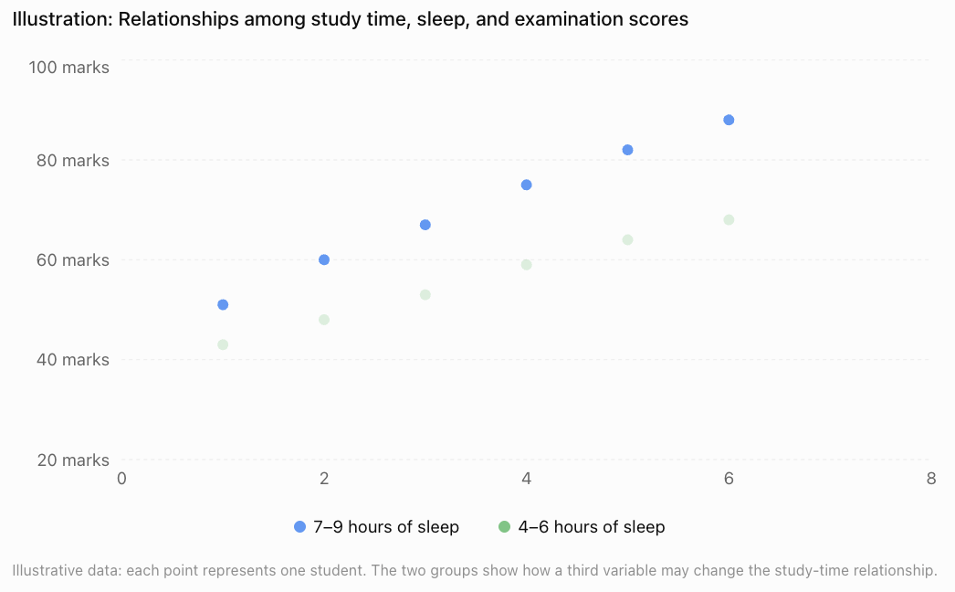
The graph suggests that both study time and sleep may be related to performance. However, it does not prove that either variable causes the differences.
Recognising Confounding Variables
A confounding variable is an additional variable that can distort the apparent relationship between an explanatory variable and an outcome.
Confounding is particularly important in observational studies.
Example: Ice cream sales and drowning incidents
Suppose a researcher discovers that months with high ice cream sales also have more drowning incidents.
Does eating ice cream cause drowning?
No.
A possible explanation is that both variables are influenced by temperature.
A confounding relationship
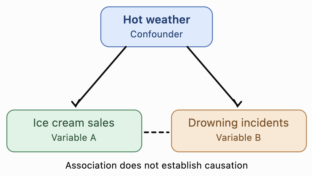
Hot weather may lead to increased ice cream purchases and more swimming activity, which can increase exposure to drowning risk.
Temperature and related seasonal conditions can therefore help explain the observed association.
Other examples of confounding
|
Observed relationship |
Possible confounding variable |
|---|---|
|
Coffee consumption and heart disease |
Smoking habits |
|
Exercise and academic performance |
General health or family resources |
|
Screen time and poor sleep |
Stress levels |
|
Education and income |
Family socioeconomic background |
|
Shoe size and reading ability in children |
Age |
These variables are possible confounders, not necessarily confirmed ones. Researchers must investigate whether they are actually associated with both variables.
How can confounding be addressed?
Researchers may use several techniques:
-
Randomisation: Randomly assign treatments to help balance confounding factors between groups.
-
Stratification: Analyse data separately within categories, such as different age groups.
-
Statistical adjustment: Include measured confounding variables in a regression model.
-
Matching: Compare individuals with similar relevant characteristics.
These methods can reduce confounding, but statistical adjustment cannot guarantee that all confounding has been eliminated.
Interpreting Multivariable Data
Multivariable datasets contain observations on several variables for each individual or object.
Consider the following hypothetical dataset.
|
Student |
Study hours |
Sleep hours |
Attendance (%) |
Exam score (%) |
|---|---|---|---|---|
|
A |
2 |
6 |
75 |
55 |
|
B |
3 |
7 |
80 |
63 |
|
C |
4 |
8 |
85 |
72 |
|
D |
5 |
7 |
90 |
78 |
|
E |
6 |
8 |
95 |
88 |
Several patterns are visible:
-
Students who study more tend to have higher examination scores.
-
Students with higher attendance also tend to have higher scores.
-
Sleep duration varies and may contribute to differences in performance.
However, the explanatory variables are themselves related. Students who study more also have higher attendance in this dataset.
This makes it difficult to determine how much each variable contributes independently.
Pairwise correlation
A correlation matrix shows the strength and direction of linear relationships between pairs of numerical variables.
Correlation coefficients range from −1 to +1.
-
r = +1: Perfect positive linear correlation.
-
r = 0: No linear correlation.
-
r = −1: Perfect negative linear correlation.
For illustration, consider this hypothetical correlation matrix.
|
Variable |
Study hours |
Sleep hours |
Attendance |
Exam score |
|---|---|---|---|---|
|
Study hours |
1.00 |
0.30 |
0.75 |
0.85 |
|
Sleep hours |
0.30 |
1.00 |
0.20 |
0.45 |
|
Attendance |
0.75 |
0.20 |
1.00 |
0.80 |
|
Exam score |
0.85 |
0.45 |
0.80 |
1.00 |
This example suggests that study hours have a strong positive linear association with examination scores.
Attendance also has a strong positive association with examination scores.
However, study hours and attendance are themselves strongly correlated.
This creates a challenge when estimating their separate contributions.
Important: A correlation matrix shows pairwise associations. It does not, by itself, account for the simultaneous effects of other variables.
Multiple Linear Regression
Multiple linear regression is a statistical technique used to model a numerical response variable using two or more explanatory variables.
The general equation is:
Where:
-
ŷ = predicted response value
-
b₀ = intercept
-
b₁, b₂, …, bₖ = regression coefficients
-
x₁, x₂, …, xₖ = explanatory variables
Each coefficient estimates the change in the predicted response associated with a one-unit increase in its explanatory variable, holding the other included explanatory variables constant.
Worked Example: Predicting Examination Scores
Suppose a statistical model predicts examination scores using study hours, sleep hours, and attendance.
The fitted equation is:
Where:
-
x₁ = study hours
-
x₂ = sleep hours
-
x₃ = attendance percentage
-
ŷ = predicted examination score
A student studies for 4 hours, sleeps for 7 hours, and has an attendance rate of 90%.
Calculate the predicted examination score.
Step 1: Write the model.
Step 2: Substitute the values.
Step 3: Calculate.
The predicted examination score is 76%.
Interpreting the coefficients
The model can also tell us how the variables are associated with examination scores.
-
Study hours (5): One additional study hour is associated with an increase of 5 percentage points in predicted score, holding sleep and attendance constant.
-
Sleep hours (2): One additional hour of sleep is associated with an increase of 2 percentage points, holding the other variables constant.
-
Attendance (0.3): A one-percentage-point increase in attendance is associated with an increase of 0.3 percentage points in predicted score, holding the other variables constant.
The intercept of 15 is the predicted score when all three explanatory variables are zero. This combination may be unrealistic, so the intercept might not have a meaningful practical interpretation.
These are model-based associations, not necessarily causal effects.
Comparing Models with Different Numbers of Variables
Adding more variables does not automatically produce a better model for prediction.
Suppose two models are available.
Model A:
This model uses only study hours.
Model B:
This model uses study hours, sleep hours, and attendance.
Model B considers more information and may provide better predictions, but this must be tested.
Adding variables can also introduce unnecessary complexity or cause the model to fit random fluctuations rather than meaningful patterns.
Evaluating model performance
Several measures help us compare statistical models.
Coefficient of determination (R²)
R² describes the proportion of variation in the observed response explained by a regression model, relative to predicting the sample mean in an ordinary least-squares model with an intercept.
For example:
R² = 0.82
This indicates that the model explains approximately 82% of the variation in examination scores within the fitted dataset.
It does not mean that the model is 82% accurate or that 82% of scores are predicted correctly.
Adjusted R²
Adjusted R² modifies R² to account for the number of explanatory variables in the model.
Unlike ordinary R², it can decrease when a new variable adds little useful explanatory information.
Root Mean Squared Error (RMSE)
RMSE measures the typical size of prediction errors, giving relatively greater weight to large errors.
Here, n is the number of observations used to calculate the errors.
A lower RMSE generally indicates smaller prediction errors when comparing models on the same outcome and evaluation dataset.
Worked Example: Comparing Model Performance
Suppose two models produce the following results on a held-out test dataset.
|
Measure |
Model A |
Model B |
|---|---|---|
|
Number of explanatory variables |
1 |
3 |
|
Test R² |
0.65 |
0.84 |
|
Test RMSE |
9.2 |
5.6 |
Model B has a higher R² and a lower RMSE.
Therefore, Model B provides better predictions on this test dataset.
However, we should still consider whether Model B is appropriate for future students, whether its relationships are stable, and whether the additional data are practical to collect.
Understanding Residuals
A residual is the difference between an observed value and the value predicted by a model.
Where:
-
y = actual value
-
ŷ = predicted value
Worked Example: Calculating Residuals
A regression model predicts the following examination scores.
|
Student |
Actual score |
Predicted score |
Residual |
|---|---|---|---|
|
A |
65 |
62 |
+3 |
|
B |
70 |
74 |
−4 |
|
C |
80 |
78 |
+2 |
|
D |
85 |
87 |
−2 |
|
E |
90 |
89 |
+1 |
For Student B:
Residual = 70 − 74 = −4
The model overestimated Student B's score by 4 percentage points.
For Student A:
Residual = 65 − 62 = +3
The model underestimated Student A's score by 3 percentage points.
Interpreting residual plots
A residual plot can reveal problems that are not obvious from R² alone.
Example of residuals with no obvious systematic pattern
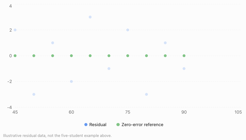
Residual patterns may reveal:
-
Curvature, suggesting that a linear model is inappropriate.
-
Increasing spread, suggesting nonconstant error variance.
-
Unusually large residuals, indicating possible outliers.
-
Clusters or trends, suggesting missing explanatory variables or other model problems.
A residual plot is useful, but it cannot prove that every model assumption is satisfied.
Multicollinearity
Multicollinearity occurs when two or more explanatory variables in a regression model are strongly linearly related.
For example, suppose a model predicts house prices using both floor area in square metres and floor area in square feet.
These variables contain essentially the same information.
This creates perfect multicollinearity, making it impossible to estimate separate coefficients for both variables in an ordinary multiple regression model.
Less extreme multicollinearity can also occur.
For example, study hours and attendance may be strongly correlated.
This can make individual coefficient estimates unstable and difficult to interpret.
Possible solutions
Researchers may:
-
Remove redundant explanatory variables.
-
Combine related variables into a meaningful index.
-
Collect additional observations with more varied combinations of predictors.
-
Use methods such as ridge regression when appropriate.
Multicollinearity is especially problematic when interpreting individual coefficients. It does not always make predictions poor.
Interaction Effects in Statistical Models
Sometimes one variable changes the relationship between another variable and the response.
This is called an interaction.
Suppose examination performance depends on both study time and access to tutoring.
A model might be:
Where:
-
x₁ = study hours
-
x₂ = tutoring status (0 = no tutoring, 1 = tutoring)
-
x₁x₂ = interaction term
Worked Example: Interpreting an Interaction
For a student without tutoring:
x₂ = 0
For a student with tutoring:
x₂ = 1
Simplifying:
The model predicts:
-
Without tutoring, each additional study hour is associated with a 5-point increase.
-
With tutoring, each additional study hour is associated with a 7-point increase.
This suggests that the relationship between study time and examination performance differs depending on tutoring status.
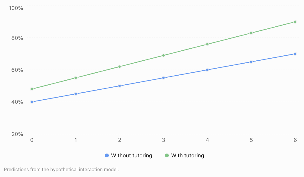
The different slopes indicate an interaction effect.
However, this hypothetical model does not establish that tutoring causes the improvement.
Choosing an Appropriate Statistical Model
Different statistical models are suitable for different types of data.
|
Situation |
Possible statistical model |
|---|---|
|
Predicting a numerical outcome from several variables |
Multiple linear regression |
|
Predicting a yes/no outcome |
Logistic regression |
|
Modelling curved relationships |
Polynomial regression or other nonlinear models |
|
Predicting counts of events |
Poisson regression |
|
Investigating time-dependent data |
Time-series models |
|
Examining repeated observations from the same individuals |
Mixed-effects models |
The choice depends on the response variable, data structure, research question, and assumptions.
Questions to ask when evaluating a model
-
Is the model suitable for the type of response variable?
-
Are the explanatory variables relevant?
-
Have important confounding variables been considered?
-
Are there strong relationships among explanatory variables?
-
Are the model assumptions reasonable?
-
Are the predictions accurate on data not used to fit the model?
-
Is the model being used within a sensible range of values?
A statistically complex model is not automatically more useful than a simpler one.
Communicating Statistical Reasoning
Statistical conclusions should be clear, accurate, and supported by evidence.
A strong statistical explanation includes the following elements.
Research question
State what the investigation is trying to determine.
Example:
"How are study time, attendance, and sleep duration associated with examination scores?"
Methods
Explain how the data were collected and analysed.
Example:
"Data from 150 students were analysed using multiple linear regression."
Results
Report relevant numerical evidence.
Example:
"The model explained 78% of the variation in examination scores in the sample (R² = 0.78)."
Interpretation
Explain what the results mean.
Example:
"After adjusting for attendance and sleep duration, study time remained positively associated with examination performance."
Limitations
Identify reasons for caution.
Example:
"The study was observational, so the results do not establish that increasing study time will cause higher examination scores. Previous achievement and motivation were not measured."
Conclusion
Provide a balanced statement that answers the original research question.
Example:
"Study time, attendance, and sleep duration were useful predictors of examination performance in this sample. Further investigation would be needed to establish causal relationships."
Avoiding misleading language
Compare the following statements.
Misleading: "Studying longer causes higher examination scores."
Better: "Students who studied longer tended to achieve higher examination scores, after accounting for the other variables included in the model."
The second statement is more appropriate when the evidence comes from an observational study.
Real-World Applications
Agriculture
Researchers investigate how sunlight, rainfall, temperature, fertiliser, and soil quality relate to crop yields. Multivariable models can help identify growing conditions associated with better harvests.
Economics and Property
Property prices can be modelled using floor area, location, age, accessibility, and nearby amenities. Analysts must consider how these predictors relate to one another.
Transport Planning
Traffic congestion can be analysed using vehicle numbers, road capacity, weather, public transport availability, and time of day.
Environmental Science
Scientists study relationships between pollution, rainfall, land use, industrial activity, and water quality to understand environmental changes.
Common Mistakes
Mistake 1: Assuming correlation proves causation
Two variables may be associated because of confounding, reverse causation, or other explanations.
Correction: Use language such as "associated with" unless the evidence supports a causal conclusion.
Mistake 2: Ignoring confounding variables
A relationship between two variables may change after accounting for a third variable.
Correction: Consider other factors that may influence both the explanatory variable and the response.
Mistake 3: Interpreting regression coefficients without considering other predictors
In multiple regression, a coefficient represents an adjusted relationship, not simply the overall pairwise association.
Correction: Interpret each coefficient while holding the other included variables constant.
Mistake 4: Assuming a higher R² always means a better model
Adding variables usually increases or preserves training R², even if the additional variables are not useful.
Correction: Consider adjusted R², residuals, and prediction performance on new data.
Mistake 5: Ignoring multicollinearity
Strong relationships among explanatory variables can make individual coefficients unstable.
Correction: Investigate redundant variables and interpret coefficients cautiously.
Mistake 6: Extrapolating beyond the observed data
A model fitted using students who study between one and six hours may produce unrealistic predictions for someone studying twenty hours.
Correction: Make predictions within the range and conditions supported by the data.
Mistake 7: Reporting statistical results without limitations
A model may work well for one dataset but poorly for another population.
Correction: Explain the sample, assumptions, uncertainty, and limitations of the conclusions.
Key Terms
-
Multiple Variable Analysis: Statistical investigation involving several variables simultaneously.
-
Response Variable: The outcome being explained or predicted.
-
Explanatory Variable: A variable used to explain or predict a response.
-
Confounding Variable: A variable associated with both the explanatory variable and the outcome that can distort their apparent relationship.
-
Correlation: A measure of the direction and strength of a relationship between variables.
-
Correlation Matrix: A table displaying pairwise correlation coefficients.
-
Multiple Linear Regression: A method for modelling a numerical response using two or more explanatory variables.
-
Regression Coefficient: A numerical value describing an estimated relationship between a predictor and the response.
-
Residual: The difference between an observed value and a predicted value.
-
R²: The coefficient of determination, measuring the proportion of variation explained by a regression model under the usual least-squares definition.
-
Adjusted R²: A version of R² that accounts for the number of explanatory variables.
-
RMSE: Root Mean Squared Error, a measure of prediction error.
-
Multicollinearity: Strong linear relationships among explanatory variables.
-
Interaction Effect: A situation where the relationship between one predictor and the response depends on another predictor.
-
Statistical Model: A mathematical representation of relationships or patterns in data.
-
Causation: A relationship in which changing one factor produces a change in another.
-
Extrapolation: Using a model to predict outside the range of the observed data.
-
Overfitting: When a model captures random features of training data rather than patterns that generalise well.
Key Takeaways
-
Real-world outcomes are often related to several variables simultaneously.
-
Multiple variable analysis helps researchers investigate these relationships more completely.
-
Confounding variables can create or distort apparent associations.
-
Correlation matrices describe pairwise relationships but do not fully account for other variables.
-
Multiple regression models estimate relationships between an outcome and several predictors.
-
Regression coefficients must be interpreted while holding other included variables constant.
-
Interaction effects occur when the relationship between one variable and the outcome depends on another variable.
-
Statistical models should be evaluated using appropriate measures of fit, prediction errors, assumptions, and residuals.
-
Multicollinearity can make individual regression coefficients difficult to interpret.
-
Strong statistical reasoning includes evidence, appropriate conclusions, and clear discussion of limitations.
Check Your Understanding
Try the following questions before examining the worked answers.
Questions
Question 1: Identifying Variables
A researcher investigates how exercise duration, sleep, and age are related to resting heart rate.
Identify the response variable and three explanatory variables.
Question 2: Confounding Variables
A study finds that people who own more books tend to achieve higher examination scores.
Identify a possible confounding variable and explain why it might influence the relationship.
Question 3: Interpreting Correlation
A dataset gives the following correlations with examination score:
-
Study hours: r = 0.82
-
Sleep duration: r = 0.35
-
Absences: r = −0.71
Which variable has the strongest linear association with examination score? Which relationship is negative?
Question 4: Multiple Regression
A model predicts examination scores using:
Where:
-
x₁ = study hours
-
x₂ = sleep hours
Calculate the predicted score for a student who studies for 5 hours and sleeps for 8 hours.
Question 5: Interpreting Coefficients
Using the model in Question 4, explain the meaning of the coefficient 6.
Question 6: Residuals
A statistical model predicts a score of 78, but the actual score is 72.
Calculate the residual and explain what it means.
Question 7: Comparing Models
Two models produce these results on the same test dataset.
|
Measure |
Model A |
Model B |
|---|---|---|
|
Test R² |
0.68 |
0.81 |
|
Test RMSE |
8.5 |
6.1 |
Which model performs better on the test dataset? Explain.
Question 8: Multicollinearity
A house-price model includes floor area measured in square metres and floor area measured in square feet.
Explain why this creates a problem.
Question 9: Interaction Effects
A model is:
Where x₂ is either 0 or 1.
Determine the relationship between ŷ and x₁ when x₂ = 0 and when x₂ = 1.
Question 10: Statistical Communication
A researcher finds that students who exercise more frequently tend to achieve higher examination scores.
Explain why the statement "Exercise causes higher examination scores" may be misleading. Write a more appropriate conclusion.
Fully Worked Answers
Answer 1: Identifying Variables
The response variable is resting heart rate, because it is the outcome being investigated.
The explanatory variables are exercise duration, sleep duration, and age.
These variables may help explain variation in resting heart rate.
Answer 2: Confounding Variables
A possible confounding variable is family socioeconomic background.
Families with greater financial resources may be able to purchase more books and provide additional educational opportunities.
This could influence both book ownership and examination performance.
Therefore, the relationship between book ownership and examination scores does not necessarily mean that owning more books causes higher scores.
Answer 3: Interpreting Correlation
Compare the absolute values of the correlation coefficients.
-
Study hours: |0.82| = 0.82
-
Sleep duration: |0.35| = 0.35
-
Absences: |−0.71| = 0.71
The strongest linear association is between study hours and examination score, because 0.82 has the greatest absolute value.
Absences have a negative correlation with examination scores.
This means students with more absences tend to have lower examination scores.
Answer 4: Multiple Regression
Given:
Substitute x₁ = 5 and x₂ = 8.
The predicted examination score is 74%.
Answer 5: Interpreting Coefficients
The coefficient 6 represents the estimated change in examination score associated with one additional hour of study, holding sleep duration constant.
Therefore, the model predicts a 6-percentage-point increase in examination score for each additional study hour, assuming the linear model is appropriate.
This does not necessarily imply that increasing study time causes the score to rise by six points.
Answer 6: Residuals
Residual = Actual − Predicted
Residual = 72 − 78
The residual is −6.
This means the model overestimated the student's examination score by 6 percentage points.
Answer 7: Comparing Models
Model B has:
-
A higher test R² (0.81 compared with 0.68).
-
A lower test RMSE (6.1 compared with 8.5).
Therefore, Model B performs better on the test dataset according to both measures.
However, we would still examine whether its assumptions are reasonable and whether its performance generalises to other students.
Answer 8: Multicollinearity
Floor area in square metres and floor area in square feet represent exactly the same physical quantity.
Their relationship is:
Area in square feet ≈ 10.764 × Area in square metres
Therefore, the two explanatory variables are perfectly linearly related.
This creates perfect multicollinearity, so an ordinary multiple regression model cannot uniquely estimate separate coefficients for both.
A sensible solution is to use only one floor-area measurement.
Answer 9: Interaction Effects
The model is:
When x₂ = 0:
The slope with respect to x₁ is 4.
When x₂ = 1:
The slope with respect to x₁ is 7.
Therefore, the relationship between x₁ and the predicted outcome differs according to the value of x₂.
This is an interaction effect.
Answer 10: Statistical Communication
The original statement is misleading because an association does not necessarily demonstrate causation.
Other factors, such as sleep, motivation, family resources, or general health, might influence both exercise habits and academic performance.
A more appropriate conclusion is:
"Students who exercised more frequently tended to achieve higher examination scores in the observed sample. However, the study does not establish that exercise directly caused the higher scores."
This conclusion accurately describes the evidence while acknowledging its limitations.
Final Reflection
Multiple variable analysis is an essential part of modern statistics because most real-world situations involve several connected factors.
A useful statistical investigation does more than identify patterns. It considers possible confounding variables, interprets the contributions of multiple predictors, evaluates model performance, and communicates conclusions without overstating what the evidence demonstrates.
The central principle is that statistical relationships must be interpreted in context. A strong model is not simply one that fits the data well, but one that produces meaningful, reliable, and appropriately qualified conclusions.
4. Statistical Modelling
Learning outcomes
- I can develop statistical models.
- I can assess model assumptions.
- I can evaluate model performance.
- I can interpret model outputs.
- I can apply models to real-world situations.
Introduction
How do scientists predict tomorrow's temperature? How do businesses estimate future sales? How can researchers investigate the factors that influence examination scores, disease rates, or population growth?
All these questions involve statistical modelling.
A statistical model is a mathematical representation of patterns and relationships in data. It allows us to describe observed behaviour, investigate relationships between variables, estimate unknown quantities, and make predictions.
Unlike a purely deterministic mathematical formula, a statistical model recognises that real-world data contain variation and uncertainty. Two students who study for the same number of hours may receive different examination scores. Two houses with similar characteristics may sell for different prices.
Statistical models help us understand these differences while identifying useful patterns.
In this lesson, we will explore how to develop statistical models, assess their assumptions, evaluate their performance, interpret their outputs, and apply them to real-world problems.
What Is a Statistical Model?
A statistical model is a mathematical description of how one or more variables are related, often including a component representing random variation.
A simple statistical model can be written as:
Where:
-
Y = observed response variable
-
X = explanatory variable
-
f(X) = systematic relationship between the variables
-
ε = random error or unexplained variation
For example, examination scores may be related to study time.
A possible model is:
This suggests that the expected examination score increases by 8 percentage points for each additional hour of study, within the range where the model is appropriate.
The error term accounts for other influences such as sleep, motivation, previous knowledge, and random variation.
Why do we use statistical models?
Statistical models can serve several purposes.
-
Description: Summarising patterns in a dataset.
-
Explanation: Investigating relationships among variables.
-
Prediction: Estimating future or unknown outcomes.
-
Inference: Drawing conclusions about a population from sample data.
-
Decision-making: Using evidence to compare possible actions.
A model designed for prediction may differ from one designed to estimate causal effects.
Developing a Statistical Model
Statistical modelling involves several connected stages.
The statistical modelling process
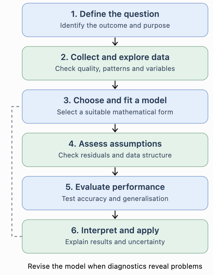
The process is iterative. Researchers often return to earlier stages after discovering problems with their data or model.
Step 1: Define the research question
Begin by identifying the outcome you want to explain or predict.
Example:
"Can examination scores be predicted using the number of hours students study?"
The response variable is examination score, and the explanatory variable is study time.
Step 2: Collect and explore data
Data should be relevant, sufficiently representative, and measured consistently.
Before fitting a model, examine:
-
Missing values and possible recording errors.
-
Unusual observations and outliers.
-
Relationships between variables.
-
Whether the data represent the intended population.
-
Whether the observations are independent or grouped.
Step 3: Choose a suitable model
The model should reflect the type of outcome and the observed pattern.
A straight-line relationship may be appropriate for some datasets, while others require nonlinear or categorical models.
Step 4: Estimate model parameters
Model parameters are numerical values that describe the relationship.
For linear regression, these include the intercept and slope.
They are estimated from data, often using the method of least squares.
Step 5: Check assumptions and performance
A model must be evaluated rather than accepted simply because it produces an equation.
Step 6: Interpret and communicate results
Explain the model in context, including its limitations and uncertainty.
Simple Linear Regression
One of the most common statistical models is simple linear regression.
It models a numerical response using one explanatory variable.
The fitted equation is:
Where:
-
ŷ = predicted response
-
a = intercept
-
b = slope
-
x = explanatory variable
Worked Example: Study Time and Examination Scores
Suppose five students produce the following data.
|
Study hours (x) |
Examination score |
|---|---|
|
1 |
48 |
|
2 |
55 |
|
3 |
61 |
|
4 |
70 |
|
5 |
76 |
We want to develop a linear model predicting examination scores from study time.
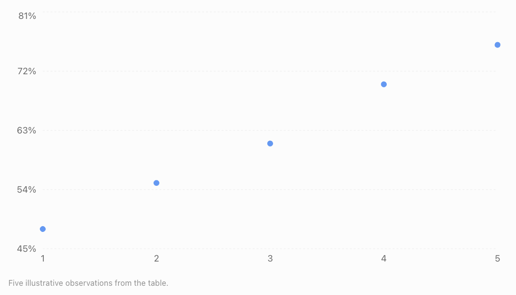
The data show a strong positive, approximately linear relationship.
Calculating the regression line
The least-squares slope is:
First calculate the means.
Now calculate the required quantities.
|
x |
y |
x − 3 |
y − 62 |
Product |
(x − 3)² |
|---|---|---|---|---|---|
|
1 |
48 |
−2 |
−14 |
28 |
4 |
|
2 |
55 |
−1 |
−7 |
7 |
1 |
|
3 |
61 |
0 |
−1 |
0 |
0 |
|
4 |
70 |
1 |
8 |
8 |
1 |
|
5 |
76 |
2 |
14 |
28 |
4 |
|
Total |
71 |
10 |
Therefore:
The intercept is:
Our fitted regression equation is:
Interpreting the model
The slope of 7.1 indicates that each additional study hour is associated with an increase of approximately 7.1 percentage points in the predicted examination score.
The intercept of 40.7 represents the predicted score at zero study hours. Because zero hours lies outside the observed range, this interpretation should be treated cautiously.
Making a prediction
For a student who studies for 4.5 hours:
The model predicts an examination score of approximately 72.7%.
This is an estimate, not a guarantee.
Choosing Different Types of Statistical Models
Different datasets require different modelling approaches.
|
Model |
Appropriate use |
Example |
|---|---|---|
|
Simple linear regression |
One numerical predictor and a numerical response |
Study time and examination score |
|
Multiple linear regression |
Several predictors and a numerical response |
House price based on size, age and location |
|
Polynomial regression |
Curved numerical relationships |
Distance travelled over time under constant acceleration |
|
Exponential regression |
Approximately constant percentage growth or decay |
Population growth |
|
Logistic regression |
Binary response |
Whether a customer makes a purchase |
|
Poisson regression |
Counts of events |
Number of calls arriving per hour |
|
Time-series model |
Data observed sequentially over time |
Monthly electricity demand |
Model selection depends on the research question, variable types, data structure, and assumptions.
Nonlinear Statistical Models
Not all relationships can be described accurately using straight lines.
Quadratic models
A quadratic model has the form:
It may describe relationships that curve upward or downward.
For example, the distance travelled by an accelerating object may follow a quadratic relationship with time.
Exponential models
An exponential model can be written as:
Where a is the initial predicted value and b is the multiplicative factor per unit increase in x.
If b is greater than 1, the model represents exponential growth.
If b is between 0 and 1, it represents exponential decay.
Example: Population Growth
Suppose a population initially contains 1,000 organisms and increases by approximately 5% each year.
A possible model is:
After 4 years:
The predicted population is approximately 1,216 organisms.
This assumes the 5% annual growth rate remains appropriate throughout the prediction period.
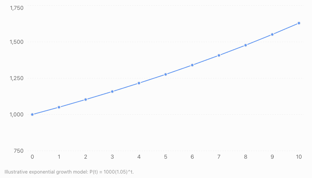
Assessing Model Assumptions
Every statistical model relies on assumptions.
If important assumptions are violated, predictions, coefficient estimates, or statistical conclusions may become unreliable.
For ordinary linear regression, several assumptions deserve particular attention.
Linearity
The expected response should have an approximately linear relationship with the explanatory variables as represented in the model.
A residual plot showing a systematic curve may suggest that the model needs nonlinear terms.
Independence
Observations or errors should satisfy the independence assumptions required by the analysis.
For example, examination scores from students in the same classroom may be related because they share a teacher and learning environment.
Ignoring this grouping can produce misleading uncertainty estimates.
Constant error variance
In standard linear regression, the spread of errors is assumed to be approximately constant across fitted values.
This is called homoscedasticity.
If the spread increases or decreases systematically, the errors exhibit heteroscedasticity.
Normality of errors
For classical small-sample regression inference, errors are commonly assumed to be normally distributed.
Normality is not required simply to calculate least-squares coefficients, and it is not the same as requiring the observed response variable itself to be normally distributed.
Multicollinearity
In multiple regression, explanatory variables should not be perfectly linearly dependent.
Strong multicollinearity can make individual coefficient estimates unstable.
Model specification
The model should include an appropriate functional form and relevant explanatory information.
Omitting important variables, using inappropriate transformations, or ignoring interactions may weaken a model.
Using Residual Plots to Assess Assumptions
A residual is the difference between an observed response and the model's prediction.
Residual plots help identify patterns that may indicate model problems.
Example A: Residuals randomly scattered around zero
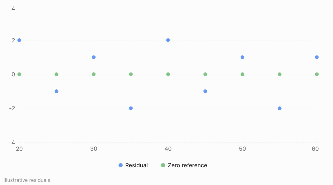
No obvious systematic pattern is visible. This is encouraging, although it does not prove that all assumptions are satisfied.
Example B: Curved residual pattern
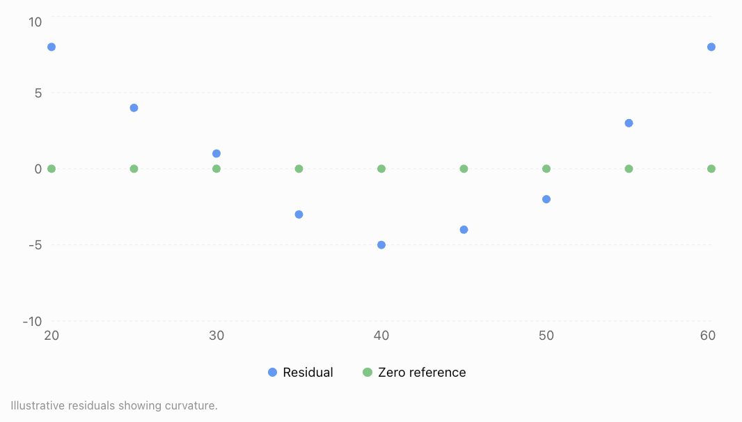
Residual plots can also show a funnel-shaped spread, suggesting nonconstant error variance.
When assumptions appear questionable, researchers may revise the model, use transformations, adopt robust inference methods, or select a different model family.
Evaluating Model Performance
A model should be judged by how well it meets its intended purpose.
For prediction, performance on previously unseen data is especially important.
Mean Absolute Error (MAE)
MAE measures the average absolute difference between observed and predicted values.
Lower values indicate smaller average absolute prediction errors.
Mean Squared Error (MSE)
MSE averages squared prediction errors.
Squaring gives greater weight to large errors.
Root Mean Squared Error (RMSE)
RMSE is the square root of MSE.
RMSE is expressed in the same units as the response variable.
Coefficient of Determination (R²)
For ordinary least-squares regression with an intercept:
Where:
-
SSres = sum of squared residuals
-
SStot = total sum of squared deviations from the observed mean
On the training dataset, R² indicates the proportion of variation explained by the model under this definition.
An R² of 0.90 means that 90% of the observed variation is accounted for by the fitted model, not that its predictions are 90% accurate.
R² on a separate test dataset can be negative when predictions perform worse than the test-set mean benchmark.
Worked Example: Calculating Prediction Errors
Suppose a model produces the following predictions.
|
Observation |
Actual |
Predicted |
Error |
Absolute error |
Squared error |
|---|---|---|---|---|---|
|
A |
50 |
52 |
−2 |
2 |
4 |
|
B |
60 |
57 |
3 |
3 |
9 |
|
C |
70 |
74 |
−4 |
4 |
16 |
|
D |
80 |
78 |
2 |
2 |
4 |
|
E |
90 |
89 |
1 |
1 |
1 |
|
Total |
12 |
34 |
Calculate MAE.
Calculate MSE.
Calculate RMSE.
The model's average absolute error is 2.4 units, while its root mean squared error is approximately 2.61 units.
RMSE is slightly larger because it gives greater weight to larger errors.
Training Data, Test Data, and Overfitting
A model may perform extremely well on the data used to build it but poorly on new observations.
This problem is called overfitting.
Training data
Training data are used to estimate model parameters.
Validation data
Validation data may be used to compare models and select settings.
Test data
Test data are held aside to provide a final assessment of predictive performance.
Example data partition

Underfitting and overfitting
Underfitting occurs when a model is too simple to capture important relationships.
Overfitting occurs when a model captures random fluctuations in training data rather than patterns that generalise.
An appropriate model balances complexity with predictive reliability.
Interpreting Model Outputs
A statistical model produces more than predictions.
It may provide coefficients, standard errors, confidence intervals, statistical tests, and measures of fit.
Consider a hypothetical multiple regression model predicting house prices in thousands of dollars.
Where:
-
A = floor area in square metres
-
G = age of the house in years
-
P = price in thousands of dollars
Interpreting coefficients
The coefficient 4.5 suggests that an additional square metre of floor area is associated with a predicted price increase of $4,500, holding house age constant.
The coefficient −1.2 suggests that each additional year of age is associated with a predicted price decrease of $1,200, holding floor area constant.
The intercept of 80 represents a predicted price of $80,000 for a property with zero floor area and zero age. This is not a realistic property, so the intercept has little practical meaning.
Worked Example: Predicting a House Price
Suppose a house has an area of 120 m² and is 15 years old.
Because the price is measured in thousands of dollars:
This prediction assumes the model is appropriate for houses with these characteristics.
Confidence intervals and prediction intervals
A confidence interval for the mean response estimates the average outcome for observations with particular explanatory-variable values.
A prediction interval estimates a range for a single new observation.
Prediction intervals are generally wider because individual outcomes contain additional variation.
For example, a model might predict a house price of $602,000, with a 95% prediction interval of $540,000 to $664,000.
The interval communicates uncertainty, although its precise interpretation depends on the statistical assumptions and method used.
Real-World Applications of Statistical Modelling
Weather Forecasting
Statistical models use historical and current atmospheric data to estimate temperatures, rainfall probabilities, and other weather conditions. Forecasts include uncertainty because atmospheric systems are complex.
Transport and Traffic
Traffic models use vehicle counts, road capacity, time of day, and weather to predict congestion and support transport planning.
Agriculture
Crop yield models investigate rainfall, soil nutrients, sunlight, temperature, and irrigation to estimate harvests and support agricultural decisions.
Business and Economics
Businesses use statistical models to forecast demand, estimate sales, investigate pricing relationships, and plan inventory.
Evaluating Whether a Model Is Appropriate
A model can have excellent numerical performance while still being unsuitable for its intended purpose.
Consider these questions:
-
Does the model answer the research question? A model that predicts accurately may not explain why a relationship occurs.
-
Are the data representative? A model trained on one population may not work for another.
-
Are important variables missing? Omitted factors may bias interpretations.
-
Are predictions being made within the observed range? Extrapolation can be unreliable.
-
Are the assumptions reasonable? Violations may affect estimates and uncertainty.
-
Does the model perform well on new data? Training performance alone is insufficient.
-
Are uncertainty and limitations communicated? Predictions should not be presented as guaranteed outcomes.
A model is useful when it is appropriate for the data, performs adequately for its purpose, and supports conclusions that can be justified.
Common Mistakes
Mistake 1: Choosing a model only because it produces a high R²
A model may fit the training data well while performing poorly on new data.
Correction: Evaluate out-of-sample performance and examine residuals.
Mistake 2: Ignoring model assumptions
A regression equation may produce misleading inferences if its assumptions are seriously violated.
Correction: Check residual patterns, independence, error variance, and other relevant assumptions.
Mistake 3: Assuming a model proves causation
Regression coefficients usually describe associations, not necessarily causal effects.
Correction: Consider study design, confounding variables, and alternative explanations.
Mistake 4: Extrapolating too far
A model developed using temperatures between 10°C and 30°C may be unreliable when predicting outcomes at 60°C.
Correction: Restrict predictions to reasonable ranges supported by the data.
Mistake 5: Confusing confidence intervals with prediction intervals
A confidence interval for the mean response is not the same as an interval for an individual future observation.
Correction: Identify the quantity whose uncertainty is being estimated.
Mistake 6: Treating predictions as exact values
Real-world observations contain unexplained variation.
Correction: Communicate prediction uncertainty and avoid unnecessary precision.
Mistake 7: Ignoring changes over time
A model based on historical conditions may become inaccurate when the underlying relationships change.
Correction: Monitor model performance and update models when appropriate.
Key Terms
-
Statistical Model: A mathematical representation of relationships and variation in data.
-
Response Variable: The outcome being explained or predicted.
-
Explanatory Variable: A variable used to explain or predict an outcome.
-
Parameter: A numerical quantity describing a statistical model.
-
Linear Regression: A method for modelling a numerical response using a linear relationship.
-
Multiple Regression: Regression involving more than one explanatory variable.
-
Nonlinear Model: A model describing relationships that are not linear in the relevant predictors or parameters.
-
Least Squares: A method that estimates parameters by minimising the sum of squared residuals.
-
Residual: The difference between an observed and predicted value.
-
Model Assumption: A condition underlying a statistical method or interpretation.
-
Homoscedasticity: Approximately constant error variance.
-
Heteroscedasticity: Nonconstant error variance.
-
MAE: Mean Absolute Error.
-
MSE: Mean Squared Error.
-
RMSE: Root Mean Squared Error.
-
R²: Coefficient of determination.
-
Training Data: Data used to fit a model.
-
Validation Data: Data used to compare or tune models.
-
Test Data: Data held aside for final predictive evaluation.
-
Overfitting: Learning random training-data fluctuations that do not generalise.
-
Underfitting: Failing to capture important relationships because a model is too simple or restrictive.
-
Cross-Validation: A technique that evaluates models across multiple training and validation splits.
-
Confidence Interval: An interval procedure used to estimate an unknown parameter or mean response with a stated confidence level.
-
Prediction Interval: An interval estimating the range of a future observation.
-
Extrapolation: Prediction beyond the range of observed data.
Key Takeaways
-
Statistical models represent patterns and relationships while accounting for uncertainty.
-
Model development begins with a clear research question and suitable data.
-
Different types of relationships require different statistical models.
-
Linear regression models numerical outcomes using linear combinations of explanatory variables.
-
Model assumptions must be examined before relying on statistical conclusions.
-
Residual plots help identify curvature, unequal error variance, and unusual observations.
-
MAE, MSE, RMSE, and R² provide different information about model performance.
-
Models should be evaluated using data not used to fit them.
-
Overfitting can produce excellent training results but poor predictions on new data.
-
Model coefficients must be interpreted in context.
-
Confidence intervals and prediction intervals describe different forms of uncertainty.
-
Statistical models support decisions but do not automatically establish causation.
Check Your Understanding
Questions
Question 1: Understanding Models
Explain what a statistical model is and why statistical models include uncertainty.
Question 2: Identifying Variables
A researcher develops a model predicting electricity consumption using outdoor temperature, household size, and the number of electrical appliances.
Identify the response variable and the explanatory variables.
Question 3: Linear Regression
A model predicts examination scores using:
Calculate the predicted score for a student who studies for 5 hours.
Question 4: Interpreting a Slope
Explain what the slope of 9 means in the model from Question 3.
Question 5: Residuals
A model predicts a house price of $450,000, but the actual selling price is $470,000.
Calculate the residual and interpret it.
Question 6: Model Performance
A model produces absolute prediction errors of 2, 4, 3, 5, and 1.
Calculate the Mean Absolute Error.
Question 7: RMSE
A model produces prediction errors of −2, 3, and −4.
Calculate the RMSE.
Question 8: Model Assumptions
A residual plot shows a clear U-shaped pattern.
What does this suggest about the model?
Question 9: Overfitting
A model achieves R² = 0.98 on its training data but R² = 0.35 on its test data.
Explain what this may indicate.
Question 10: Model Selection
A researcher wants to predict whether a student will pass or fail an examination using attendance and study time.
Which type of model would be suitable, and why?
Question 11: Exponential Modelling
A population begins with 500 organisms and grows by 8% annually.
Write an exponential model and predict the population after 3 years.
Question 12: Statistical Reasoning
A statistical model finds a positive relationship between social media use and anxiety scores.
Explain why the researcher should not automatically conclude that social media use causes anxiety.
Fully Worked Answers
Answer 1: Understanding Models
A statistical model is a mathematical representation of patterns or relationships in data.
Statistical models include uncertainty because real-world outcomes are influenced by many factors, including variables not included in the model, measurement error, and random variation.
Therefore, a model usually provides estimates rather than exact outcomes.
Answer 2: Identifying Variables
The response variable is electricity consumption.
The explanatory variables are outdoor temperature, household size, and the number of electrical appliances.
These factors may help explain differences in electricity consumption between households.
Answer 3: Linear Regression
The model is:
Substitute x = 5.
The predicted examination score is 80%.
Answer 4: Interpreting a Slope
The slope is 9.
This means that each additional hour of study is associated with a predicted increase of 9 percentage points in examination score.
This interpretation assumes the linear model is appropriate over the relevant range.
It does not necessarily establish that studying one additional hour causes a nine-point increase.
Answer 5: Residuals
Residual = Actual − Predicted
The residual is positive.
Therefore, the model underestimated the house price by $20,000.
Answer 6: Model Performance
MAE is the mean of the absolute errors.
The average absolute prediction error is 3 units.
Answer 7: RMSE
The errors are −2, 3, and −4.
First square each error.
Calculate the mean squared error.
Take the square root.
The RMSE is approximately 3.11 units.
Answer 8: Model Assumptions
A U-shaped residual pattern suggests that the model may not be capturing a curved relationship.
For example, a straight-line model may have been fitted to data that follow a quadratic pattern.
The researcher should investigate nonlinear terms or a more appropriate model.
Answer 9: Overfitting
The model explains much of the variation in the training data but performs substantially worse on the test data.
This may indicate overfitting.
The model may have captured random fluctuations in the training data rather than generalisable relationships.
Possible improvements include reducing unnecessary complexity, collecting more representative data, and using cross-validation for model selection.
Answer 10: Model Selection
A logistic regression model would be suitable.
The response variable has two possible outcomes:
-
Pass
-
Fail
Logistic regression models the probability of a binary outcome using explanatory variables such as attendance and study time.
It can estimate the probability that a student passes rather than directly predicting an unrestricted numerical examination score.
Answer 11: Exponential Modelling
The initial population is 500.
The annual growth rate is 8%.
The exponential model is:
After 3 years:
The predicted population after three years is approximately 630 organisms.
Answer 12: Statistical Reasoning
A positive association between social media use and anxiety scores does not automatically demonstrate causation.
Other factors, such as stress, sleep patterns, or social circumstances, may influence both variables.
Reverse causation is also possible: people experiencing anxiety may use social media more frequently.
A more appropriate conclusion would be:
"Greater social media use was associated with higher anxiety scores in the observed sample. Further research is needed to determine whether a causal relationship exists."
Final Reflection
Statistical modelling connects mathematical reasoning with real-world evidence. It allows researchers to move beyond simply describing data and begin investigating relationships, making predictions, and evaluating possible explanations.
However, a useful statistical model is not necessarily the most complicated model or the one with the highest training R². It is a model that addresses the research question, makes reasonable assumptions, performs reliably, and produces conclusions that are supported by the evidence.
The most important skill is not simply calculating a regression equation. It is understanding what the model tells us, what it cannot tell us, and how confidently we can use its results.
5. Communicating Statistical Results
Learning outcomes
- I can present statistical findings clearly.
- I can justify conclusions using evidence.
- I can create effective statistical reports.
- I can evaluate the quality of statistical investigations.
- I can apply statistical thinking to solve authentic problems.
Introduction
Imagine that a school conducts a survey to investigate whether students who sleep longer achieve higher examination scores. After collecting data from 200 students, the researchers discover a positive relationship between sleep duration and academic performance.
But how should they communicate this discovery?
Should they simply announce that students who sleep longer achieve better grades? Should they present a table containing all 200 observations? Or should they use graphs, statistical summaries, and carefully explained conclusions?
Collecting and analysing data are only part of a statistical investigation. The results must also be communicated in ways that are clear, accurate, meaningful, and supported by evidence.
Statistical communication involves selecting appropriate graphs and numerical summaries, explaining patterns, justifying conclusions, acknowledging uncertainty, and making recommendations based on reliable evidence.
These skills are essential in science, business, education, medicine, economics, environmental research, and public policy.
A well-communicated statistical investigation allows readers to understand not only what the data suggest, but also how the conclusions were reached and how much confidence should be placed in them.
The Purpose of Statistical Communication
Statistical communication is the process of presenting data, analyses, interpretations, and conclusions so that an audience can understand and evaluate them.
Effective statistical communication answers five important questions:
-
What was investigated? State the research question and purpose.
-
How was the investigation conducted? Explain the data collection and analysis methods.
-
What did the data show? Present important numerical results and visualisations.
-
What do the results mean? Interpret the findings in context.
-
How reliable are the conclusions? Discuss uncertainty, limitations, and possible sources of error.
Statistical communication should be understandable without oversimplifying or misrepresenting the evidence.
Description, interpretation, and conclusion
These three elements serve different purposes.
Consider a hypothetical investigation of study time and examination performance.
|
Element |
Example |
|---|---|
|
Description |
The correlation between study hours and examination scores was r = 0.78. |
|
Interpretation |
Students who studied longer tended to achieve higher examination scores. |
|
Conclusion |
Study time was strongly associated with examination performance, although the investigation does not establish causation. |
A statistical report should distinguish clearly between what was observed and what can reasonably be concluded.
Presenting Statistical Findings Clearly
The most effective way to present statistical information depends on the type of data, the purpose of the analysis, and the intended audience.
Choosing appropriate graphs
|
Graph type |
Best used for |
|---|---|
|
Bar chart |
Comparing frequencies or values across categories |
|
Histogram |
Showing the distribution of continuous numerical data |
|
Box plot |
Comparing medians, quartiles, and spread |
|
Scatter plot |
Investigating relationships between two numerical variables |
|
Line graph |
Showing changes over time |
|
Dot plot |
Displaying individual numerical observations |
|
Error-bar graph |
Showing estimates together with variability or uncertainty |
Graphs should make important relationships easier to understand, not simply make a report more colourful.
Example: Comparing examination results
Suppose two classes complete the same examination.
|
Statistic |
Class A |
Class B |
|---|---|---|
|
Number of students |
30 |
30 |
|
Mean score |
72 |
78 |
|
Median score |
73 |
79 |
|
Standard deviation |
10 |
7 |
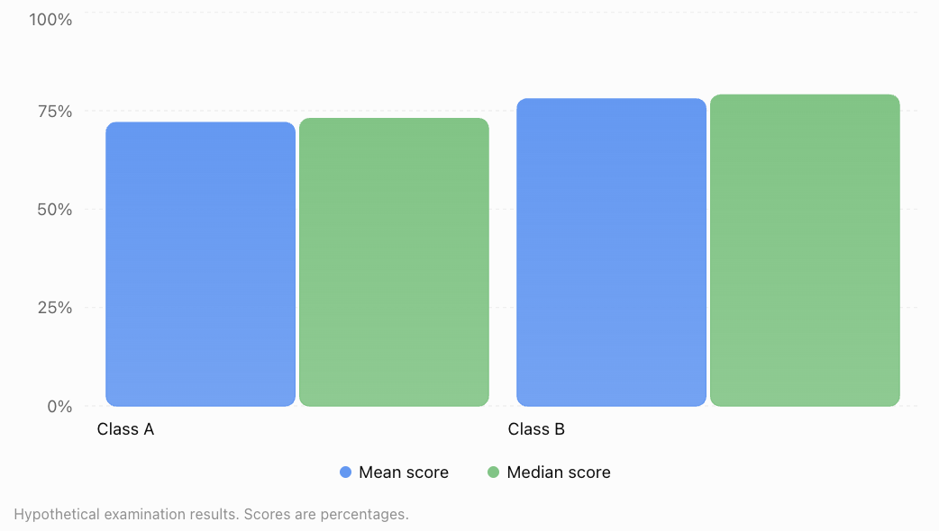
A suitable description is:
"Class B achieved a higher mean examination score (78%) than Class A (72%). Class B also had a lower standard deviation (7 compared with 10 percentage points), indicating less variation in scores as measured by standard deviation."
This statement identifies both the difference in average performance and the difference in variability.
It does not claim that Class B's teacher or teaching method caused the difference.
Principles of effective graphs
A well-designed statistical graph should:
-
Have a clear, informative title.
-
Label axes and include measurement units.
-
Use an appropriate scale.
-
Distinguish groups clearly.
-
Avoid unnecessary decoration.
-
Include sample sizes when relevant.
-
Explain uncertainty where appropriate.
-
Accurately represent the underlying data.
For bar charts, a zero baseline is generally important because bar length represents magnitude. Scatter plots and line graphs may use narrower scales when clearly labelled and appropriate.
Avoiding Misleading Statistical Visualisations
Graphs can influence how an audience interprets results.
Poor graph design may exaggerate differences, hide variation, or suggest relationships that are not supported by the data.
Example: Misleading axis scales
Suppose a company's sales increase from $100,000 to $110,000.
The actual percentage increase is:
A bar chart beginning at $95,000 could make the difference appear enormous because the second bar would be three times the visible height of the first.
A bar chart beginning at zero represents the relative magnitudes more faithfully.
Same data, different visual impressions
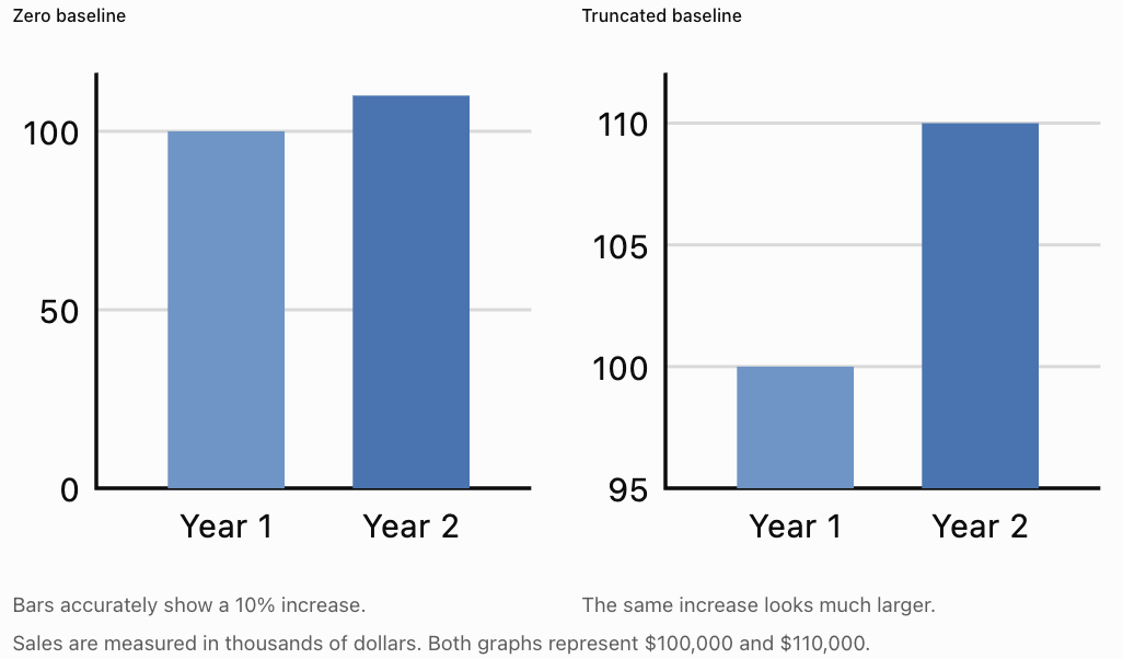
Other misleading practices include using unequal intervals on axes without explanation, presenting percentages without sample sizes, omitting relevant categories, and using three-dimensional effects that distort visual comparisons.
Justifying Conclusions Using Statistical Evidence
A statistical conclusion should follow logically from the evidence.
A strong conclusion combines:
Claim + Evidence + Statistical Reasoning + Qualification
Worked Example: Does Study Time Relate to Examination Performance?
A researcher collects data from 80 students and reports:
-
Mean study time: 4.2 hours per week.
-
Mean examination score: 74%.
-
Pearson correlation coefficient: r = 0.76.
-
Fitted regression equation: ŷ = 48 + 6.2x.
The correlation of 0.76 indicates a strong positive linear association.
The regression slope suggests that each additional study hour per week is associated with an increase of approximately 6.2 percentage points in the predicted examination score, within the model's relevant range.
A justified conclusion is:
"The investigation found a strong positive linear association between weekly study time and examination performance (r = 0.76). The fitted regression model predicted an increase of approximately 6.2 percentage points in examination score for each additional study hour per week. However, the observational study cannot establish that increasing study time causes higher scores."
This conclusion is stronger than simply stating that studying improves grades because it reports evidence and acknowledges limitations.
Statistical significance and practical significance
Statistical significance and practical importance are not the same.
A very small difference may be statistically significant in a large sample but have little real-world importance.
For example, a new teaching method might increase average examination scores by 0.4 percentage points.
Even if the difference is statistically significant, a school must consider whether such a small improvement justifies the additional cost or effort.
A good report therefore considers:
-
The estimated size of the effect.
-
The uncertainty surrounding the estimate.
-
Statistical significance where appropriate.
-
Practical importance.
-
The context in which decisions will be made.
Communicating Uncertainty
Statistical conclusions are rarely completely certain.
Data are affected by sampling variation, measurement error, missing information, and other sources of uncertainty.
Confidence intervals
A confidence interval provides a range of plausible values for an unknown population parameter using a procedure with a stated long-run coverage rate.
For example, suppose a survey estimates that 62% of students prefer online homework, with a 95% confidence interval from 57% to 67%.
A suitable interpretation is:
"The estimated proportion of students who prefer online homework is 62%, with a 95% confidence interval from 57% to 67%."
The 95% confidence level describes the long-run performance of the interval procedure, not a 95% probability assigned to the fixed population proportion after the interval has been calculated.
Margin of error
For a symmetric interval:
Using the example:
The margin of error is 5 percentage points.
The result can be presented as:
This uncertainty measure addresses sampling variability under the relevant assumptions. It does not automatically account for selection bias or inaccurate responses.
Creating Effective Statistical Reports
A statistical report should present an investigation in a logical sequence so that another person can understand and evaluate it.
Recommended report structure
|
Section |
Purpose |
|---|---|
|
Title |
Identifies the investigation |
|
Executive summary or abstract |
Summarises the purpose, methods, findings, and conclusions |
|
Introduction |
Explains the research question and context |
|
Methodology |
Describes sampling, data collection, and analysis |
|
Results |
Presents graphs, tables, and statistical calculations |
|
Discussion |
Interprets findings and compares possible explanations |
|
Limitations |
Identifies uncertainty, bias, and weaknesses |
|
Conclusion |
Answers the research question using evidence |
|
Recommendations |
Suggests justified actions or further research |
|
References and appendix |
Documents sources and supporting calculations |
Example: A short statistical report
Student Sleep and Academic Performance
Illustrative statistical investigation
Research Question
Is sleep duration associated with examination performance among secondary school students?
Methodology
A hypothetical sample of 120 students reported their average nightly sleep duration. Examination scores were obtained from a common assessment. The relationship was investigated using a scatter plot and Pearson correlation.
Results
The mean sleep duration was 7.1 hours, and the mean examination score was 73%. The correlation coefficient was r = 0.48, indicating a moderate positive linear association.
Discussion
Students reporting longer sleep duration tended to achieve higher examination scores. However, study habits, stress, health, and previous achievement may also influence academic performance.
Limitations
Sleep duration was self-reported, and the sample may not represent all secondary school students. The observational design does not establish causation.
Conclusion
The results suggest a positive association between sleep duration and examination performance in the sample. Further investigation would be needed before making causal claims.
This example illustrates how a report can communicate useful findings without overstating the evidence.
Writing Clear Statistical Explanations
Statistical language should be precise but accessible.
Compare these statements.
|
Less effective statement |
Improved statement |
|---|---|
|
Scores were better. |
The mean score increased from 68% to 75%. |
|
There was a big relationship. |
The variables showed a strong positive linear correlation (r = 0.84). |
|
The new method worked. |
Students using the new method achieved a higher mean score, although other explanations remain possible. |
|
The model was very accurate. |
The model achieved a test-set RMSE of 4.2 percentage points. |
|
The result proves the hypothesis. |
The findings provide evidence consistent with the hypothesis. |
Adapting communication to the audience
Different audiences require different levels of detail.
A school principal may want a brief explanation of examination trends and recommendations.
A statistics teacher may want the sampling method, calculations, graphs, and assumptions.
A scientific researcher may require confidence intervals, model diagnostics, and detailed methodology.
The underlying results should remain consistent, even when the level of explanation changes.
Evaluating the Quality of Statistical Investigations
A statistical investigation must be evaluated before its conclusions are accepted.
Several factors determine its quality.
Sampling quality
A representative sample should reflect the population being studied.
For example, a survey about all students at a school should not rely exclusively on members of one sports team.
Sample size
Larger samples often reduce random sampling uncertainty, but a large biased sample can still produce misleading conclusions.
Sample size alone does not guarantee quality.
Measurement reliability
Measurements should be consistent and sufficiently accurate.
A survey asking students to estimate their sleep duration from memory may contain reporting errors.
Confounding variables
A third variable may influence both the explanatory variable and the outcome.
For example, family resources might be related to both access to tutoring and examination performance.
Appropriate statistical methods
Researchers should use methods suited to the variables, sampling design, and research question.
For example, Pearson correlation measures linear association between numerical variables. It is not automatically appropriate for every type of dataset.
Transparency and reproducibility
A good investigation explains how data were collected, cleaned, analysed, and interpreted.
Another researcher should be able to understand and, where practical, reproduce the analysis.
Worked Example: Evaluating a Survey
A company claims:
"Nine out of ten customers prefer our new product."
The claim is based on an online survey completed by 20 customers who voluntarily responded after receiving a promotional email.
Evaluate the investigation.
Step 1: Examine the sample size.
Only 20 people responded. This is a small sample for making broad claims about all customers.
Step 2: Consider sampling bias.
Customers who chose to respond may have stronger opinions than those who did not.
Step 3: Examine representativeness.
The respondents may not represent the company's entire customer base.
Step 4: Consider the wording of the question.
A leading question could influence responses.
Step 5: Form a justified conclusion.
The survey shows that 18 of the 20 respondents preferred the new product.
It does not provide strong evidence that 90% of all customers prefer it.
A better statement would be:
"Of the 20 customers who responded to our voluntary survey, 18 preferred the new product. A larger, more representative survey is needed to estimate preferences across the full customer population."
Applying Statistical Thinking to Authentic Problems
Statistical thinking involves using evidence and uncertainty to investigate problems and make informed decisions.
Application 1: Reducing electricity consumption
A school wants to reduce electricity use.
Researchers collect data on daily electricity consumption, outdoor temperature, classroom occupancy, and air-conditioning hours.
They may use multiple regression to investigate which variables are associated with higher electricity consumption.
A useful recommendation might be to test adjusted air-conditioning schedules, but the school should evaluate the effects of the changes rather than assume that observed associations establish causation.
Application 2: Improving transport efficiency
A city wants to reduce traffic congestion.
Researchers examine traffic volume, travel time, weather, road capacity, and public transport use.
Statistical models can identify recurring congestion patterns and support comparisons of transport strategies.
However, predictions should be evaluated against observed traffic conditions, particularly after major road or policy changes.
Application 3: Improving crop production
An agricultural researcher investigates how rainfall, fertiliser, temperature, and soil quality relate to crop yield.
A statistical model may reveal that fertiliser is positively associated with crop yield up to a certain point, after which the benefits become smaller.
This could support further experiments to identify an effective fertiliser application rate.
A Complete Statistical Investigation: Worked Case Study
A school wants to determine whether a new revision programme is associated with improved mathematics results.
Two groups of 40 students take the same final assessment.
|
Statistic |
Revision programme |
Standard revision |
|---|---|---|
|
Sample size |
40 |
40 |
|
Mean score |
78 |
72 |
|
Standard deviation |
8 |
10 |
Assume the students were independently sampled and that the groups are independent.
Step 1: Identify the research question
Is there evidence that average mathematics performance differs between students using the new revision programme and those using standard revision?
Step 2: Calculate the difference in sample means
The revision-programme group achieved a mean score 6 percentage points higher.
Step 3: Estimate the standard error
For independent groups, the estimated standard error of the difference in means is:
Substitute:
Step 4: Calculate an approximate 95% confidence interval
Using a Welch two-sample t approach, the degrees of freedom are approximately 74 and the 95% critical value is approximately 1.99.
The estimated difference in population mean scores is approximately 2.0 to 10.0 percentage points, with a 95% confidence interval under the stated sampling assumptions.
Step 5: Interpret the evidence
The confidence interval does not contain zero, suggesting evidence of a difference in population mean examination scores under the model assumptions.
However, the investigation has not stated whether students were randomly assigned to the revision methods.
If the groups differed in prior achievement, motivation, or other factors, these differences could partly explain the result.
Step 6: Communicate the conclusion
"The revision-programme group achieved a mean examination score of 78%, compared with 72% for the standard-revision group. The estimated mean difference was 6 percentage points, with an approximate 95% confidence interval of 2.0 to 10.0 percentage points. The results provide evidence of higher average performance in the revision-programme group, although further information about group assignment and possible confounding variables is needed before attributing the difference to the programme itself."
This is an evidence-based conclusion because it includes the effect size, uncertainty, and limitations.
Common Mistakes
Mistake 1: Presenting results without context
A statistic such as "r = 0.72" is not meaningful to every reader.
Correction: Explain what the statistic measures and what it suggests in the investigation.
Mistake 2: Using inappropriate or misleading graphs
Truncated bar charts, missing labels, or unsuitable graph types may distort interpretation.
Correction: Choose visualisations that represent the data accurately.
Mistake 3: Confusing correlation with causation
An observed association does not automatically demonstrate that one variable causes another.
Correction: Consider confounding, reverse causation, and study design.
Mistake 4: Ignoring uncertainty
Reporting a sample estimate as though it were the exact population value can mislead readers.
Correction: Include confidence intervals, margins of error, or other appropriate uncertainty measures.
Mistake 5: Reporting statistical significance without effect size
A statistically significant result may have little practical importance.
Correction: Report the size and context of the effect.
Mistake 6: Overgeneralising from a biased sample
Results from a convenience sample may not represent the wider population.
Correction: Explain how the sample was selected and who the conclusions apply to.
Mistake 7: Making recommendations stronger than the evidence supports
A small observational study may identify a possible relationship without proving an intervention will work.
Correction: Match recommendations to the strength and limitations of the evidence.
Mistake 8: Omitting methodology
Readers cannot adequately evaluate an investigation if they do not know how the data were obtained.
Correction: Clearly describe sampling, measurements, analysis, and assumptions.
Key Terms
-
Statistical Communication: Presenting statistical information clearly, accurately, and meaningfully.
-
Statistical Report: A structured document explaining a statistical investigation and its findings.
-
Research Question: The question an investigation aims to answer.
-
Descriptive Statistics: Numerical summaries such as means, medians, and standard deviations.
-
Statistical Inference: Drawing conclusions about populations using sample data.
-
Evidence-Based Conclusion: A conclusion supported by relevant data and statistical reasoning.
-
Effect Size: A measure of the magnitude of a relationship or difference.
-
Statistical Significance: Evidence against a null hypothesis assessed using a statistical test and significance criterion.
-
Practical Significance: The real-world importance of a statistical result.
-
Confidence Interval: An interval estimate constructed using a procedure with a stated long-run coverage probability.
-
Margin of Error: A quantity describing the half-width of a symmetric interval estimate.
-
Sampling Bias: Systematic distortion caused by how observations are selected.
-
Response Bias: Systematic distortion caused by inaccurate or influenced responses.
-
Confounding Variable: A variable that can distort an apparent relationship between other variables.
-
Correlation: A measure of association between variables.
-
Causation: A relationship in which changing one factor produces a change in another.
-
Representativeness: The extent to which a sample reflects its intended population.
-
Reliability: The consistency of a measurement or procedure.
-
Validity: The extent to which a method measures or supports what it is intended to measure or infer.
-
Reproducibility: The ability to obtain consistent results by repeating an analysis using the same data and methods.
-
Data Visualisation: Graphical representation of information and statistical patterns.
Key Takeaways
-
Statistical findings must be communicated clearly and accurately.
-
Effective communication includes the research question, methods, results, interpretation, and limitations.
-
Graphs should be chosen according to the data and should avoid misleading scales or representations.
-
Statistical conclusions must be justified using numerical evidence and sound reasoning.
-
Description, interpretation, and causal conclusions are different.
-
Confidence intervals and other uncertainty measures help communicate the precision of estimates.
-
Statistical significance does not automatically imply practical importance.
-
Effective statistical reports are structured, transparent, and understandable to their intended audience.
-
Investigations should be evaluated for sampling quality, measurement reliability, appropriate analysis, and potential bias.
-
Statistical thinking supports authentic decision-making by combining evidence with uncertainty and context.
Check Your Understanding
Questions
Question 1: Statistical Communication
Explain why presenting a statistical result without context can be misleading.
Question 2: Choosing a Graph
Choose the most appropriate graph for each situation.
a) Comparing the number of students in four school clubs.
b) Investigating the relationship between study hours and examination scores.
c) Showing monthly electricity consumption over two years.
d) Comparing the distribution of examination scores across three classes.
Question 3: Interpreting Evidence
A study finds a correlation of r = −0.82 between the number of absences and examination scores.
Describe the relationship and explain what cannot be concluded from this result alone.
Question 4: Percentage Change
A school increases its recycling rate from 40% to 50%.
Calculate:
a) The increase in percentage points.
b) The percentage increase relative to the original recycling rate.
Question 5: Confidence Intervals
A survey estimates that 64% of students support a new school timetable, with a 95% confidence interval from 59% to 69%.
State the estimated proportion, calculate the margin of error, and explain the interval appropriately.
Question 6: Evaluating a Survey
A school surveys 25 students from its mathematics club to estimate how many students across the school enjoy mathematics.
Identify two weaknesses in this investigation.
Question 7: Justifying a Conclusion
Two classes complete the same examination.
Class A has a mean score of 75%, while Class B has a mean score of 69%.
Write a justified conclusion and explain what additional information would help evaluate the difference.
Question 8: Statistical Significance
A new teaching method increases the average examination score by 0.3 percentage points in a very large study, and the difference is statistically significant.
Explain why the school should still consider practical significance.
Question 9: Evaluating a Claim
A company reports that its product is preferred by 90% of customers, based on 18 positive responses from 20 volunteers.
Explain why this claim may be misleading.
Question 10: Authentic Problem Solving
A school wants to reduce food waste in its cafeteria.
Describe a statistical investigation that could help the school make an evidence-based decision. Include the research question, data collection, analysis, and communication of findings.
Fully Worked Answers
Answer 1: Statistical Communication
A statistical result without context may be difficult to interpret or may create a misleading impression.
For example, saying "Scores increased by 10%" does not explain the original score, the final score, the sample size, or how the data were collected.
A clearer statement would be:
"The mean examination score increased from 60% to 66%, representing a relative increase of 10%, or 6 percentage points."
Context allows readers to understand the magnitude and meaning of the result.
Answer 2: Choosing a Graph
a) Bar chart, because the data involve categories of school clubs.
b) Scatter plot, because the investigation examines a relationship between two numerical variables.
c) Line graph, because electricity consumption is measured sequentially over time.
d) Side-by-side box plots, because these allow comparison of medians, quartiles, spread, and possible outliers across classes.
Answer 3: Interpreting Evidence
The correlation coefficient is r = −0.82.
This indicates a strong negative linear association.
Students with more absences tend to have lower examination scores.
However, the result does not establish that absences cause lower scores.
Other factors, such as illness, family circumstances, or learning difficulties, may influence both attendance and performance.
Answer 4: Percentage Change
Part a: Percentage-point increase
Part b: Relative percentage increase
The recycling rate increased by 10 percentage points, representing a 25% relative increase.
These two measures describe different aspects of the same change.
Answer 5: Confidence Intervals
The estimated proportion is 64%.
The confidence interval is 59% to 69%.
Calculate the margin of error:
The margin of error is 5 percentage points.
The result can be expressed as:
The 95% confidence level means that, under the statistical assumptions, the interval-building procedure would contain the true population proportion in approximately 95% of repeated samples.
It does not guarantee that the particular interval is correct, nor does it account for all possible sampling biases.
Answer 6: Evaluating a Survey
Two weaknesses are:
Selection bias: Students in the mathematics club are likely to have a greater interest in mathematics than the average student.
Small and potentially unrepresentative sample: Only 25 students were surveyed, and they were all selected from one particular group.
A better investigation would use a larger, appropriately selected sample from across the school.
Answer 7: Justifying a Conclusion
A suitable conclusion is:
"Class A achieved a mean examination score of 75%, compared with 69% for Class B. The observed difference was 6 percentage points."
To evaluate the difference more fully, we would need information about sample sizes, variation in scores, previous achievement, and whether the classes were comparable.
The difference in sample means alone does not establish statistical significance or explain why the groups performed differently.
Answer 8: Statistical Significance
Statistical significance indicates that the observed result is inconsistent with the null hypothesis to a degree specified by the statistical test and significance level.
However, an increase of only 0.3 percentage points may have little educational importance.
The school should consider whether the improvement justifies the time, cost, and resources required by the new teaching method.
Therefore, statistical significance and practical significance must be evaluated separately.
Answer 9: Evaluating a Claim
The calculation is:
The numerical statement is correct for the 20 respondents.
However, the sample is small and consists of volunteers, who may not represent the wider customer population.
Therefore, the company should not confidently generalise the 90% figure to all customers.
A more accurate statement would be:
"Of the 20 volunteers surveyed, 18 preferred the product."
Answer 10: Authentic Problem Solving
Research question
"How much food is wasted in the school cafeteria, and which factors are associated with higher waste levels?"
Data collection
Measure the mass of food waste each day over several weeks. Record the menu, number of meals served, portion sizes, and relevant student feedback.
Analysis
Calculate average food waste per meal, compare waste across different menu types, and investigate relationships between portion size and waste.
Graphs could show daily waste trends and comparisons between meal categories.
Communication
Prepare a report including the research question, methodology, numerical summaries, graphs, conclusions, and limitations.
Recommendation
If larger portions are consistently associated with more waste, the school could trial optional smaller portions.
The school should then collect new data to evaluate whether the change actually reduces food waste.
This is an example of using statistical thinking to investigate a practical problem, develop a possible solution, and evaluate its effectiveness.
Final Reflection
Communicating statistical results is more than presenting numbers or drawing graphs. It involves transforming data into evidence that people can understand, question, and use.
An effective statistical investigation should make it possible for readers to identify the research question, understand the methods, evaluate the results, and judge whether the conclusions are justified.
The most important principle is that the strength of a statistical conclusion must never exceed the strength of the evidence supporting it.
When statistical findings are communicated clearly, accurately, and responsibly, they become powerful tools for solving problems and making informed decisions.