Regression, Correlation, and Statistical Modelling
3. Multiple Variable Analysis
Learning outcomes
- I can identify relationships among multiple variables.
- I can recognise confounding variables.
- I can interpret multivariable data.
- I can evaluate statistical models.
- I can communicate statistical reasoning.
Introduction
In many real-world situations, an outcome is influenced by several factors at the same time. A student's examination score might depend on study time, attendance, sleep, and previous knowledge. The price of a house might depend on its size, location, age, and condition. Scientists studying plant growth might investigate sunlight, water, temperature, and soil nutrients.
Multiple variable analysis is the process of investigating relationships among three or more variables. Rather than examining only one possible influence, we consider how several variables interact and contribute to an outcome.
This approach helps us identify important relationships, recognise misleading conclusions, make predictions, and evaluate statistical evidence.
By the end of this lesson, you will be able to identify relationships among multiple variables, recognise confounding variables, interpret multivariable data, evaluate statistical models, and communicate statistical reasoning clearly.
Understanding Multiple Variables
A variable is a characteristic or quantity that can change or take different values.
In a statistical investigation, variables often have different roles.
-
Response variable (dependent variable): The outcome we want to explain or predict.
-
Explanatory variable (independent variable): A variable that may help explain changes in the response.
-
Control variable: A variable deliberately kept constant in an experiment.
-
Confounding variable: A variable that complicates the interpretation of a relationship because it is associated with both the explanatory variable and the outcome.
Consider a study investigating examination performance.
|
Variable |
Possible role |
|---|---|
|
Examination score |
Response variable |
|
Hours spent studying |
Explanatory variable |
|
Attendance percentage |
Additional explanatory variable |
|
Hours of sleep |
Additional explanatory variable |
|
Previous academic achievement |
Potential confounding variable |
A simple analysis might compare examination scores with study time.
A multiple variable analysis considers study time, attendance, sleep, and previous achievement together.
This provides a more complete picture of student performance.
Identifying Relationships Among Multiple Variables
When analysing multiple variables, we look for patterns that explain how variables are related.
Positive relationships
A positive relationship occurs when higher values of one variable tend to be associated with higher values of another.
For example:
-
More study time may be associated with higher examination scores.
-
Greater work experience may be associated with higher salaries.
-
Higher temperatures may be associated with greater electricity use for cooling.
Negative relationships
A negative relationship occurs when higher values of one variable tend to be associated with lower values of another.
For example:
-
Greater distance from a city centre may be associated with lower property prices.
-
More hours of exercise may be associated with a lower resting heart rate.
-
Higher product prices may be associated with lower demand.
Nonlinear relationships
Not all relationships follow straight lines.
For example, examination scores may improve rapidly with additional study time initially, but the benefits may become smaller after many hours.
A model that assumes a constant increase might therefore be inappropriate.
Relationships involving interactions
Sometimes the relationship between two variables depends on a third variable.
For example, the effect of study time on examination scores might depend on sleep duration.
Students who study for four hours but sleep very little may perform differently from students who study for four hours and get sufficient sleep.
This is called an interaction effect.
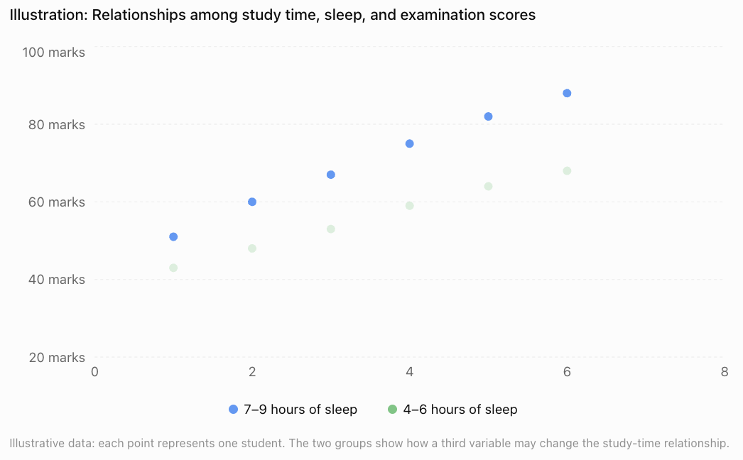
The graph suggests that both study time and sleep may be related to performance. However, it does not prove that either variable causes the differences.
Recognising Confounding Variables
A confounding variable is an additional variable that can distort the apparent relationship between an explanatory variable and an outcome.
Confounding is particularly important in observational studies.
Example: Ice cream sales and drowning incidents
Suppose a researcher discovers that months with high ice cream sales also have more drowning incidents.
Does eating ice cream cause drowning?
No.
A possible explanation is that both variables are influenced by temperature.
A confounding relationship
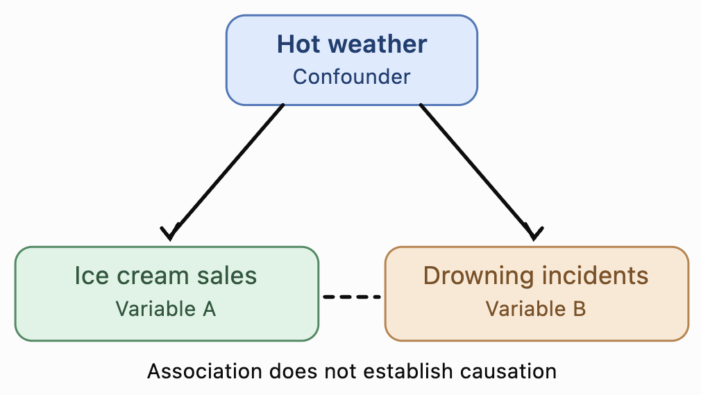
Hot weather may lead to increased ice cream purchases and more swimming activity, which can increase exposure to drowning risk.
Temperature and related seasonal conditions can therefore help explain the observed association.
Other examples of confounding
|
Observed relationship |
Possible confounding variable |
|---|---|
|
Coffee consumption and heart disease |
Smoking habits |
|
Exercise and academic performance |
General health or family resources |
|
Screen time and poor sleep |
Stress levels |
|
Education and income |
Family socioeconomic background |
|
Shoe size and reading ability in children |
Age |
These variables are possible confounders, not necessarily confirmed ones. Researchers must investigate whether they are actually associated with both variables.
How can confounding be addressed?
Researchers may use several techniques:
-
Randomisation: Randomly assign treatments to help balance confounding factors between groups.
-
Stratification: Analyse data separately within categories, such as different age groups.
-
Statistical adjustment: Include measured confounding variables in a regression model.
-
Matching: Compare individuals with similar relevant characteristics.
These methods can reduce confounding, but statistical adjustment cannot guarantee that all confounding has been eliminated.
Interpreting Multivariable Data
Multivariable datasets contain observations on several variables for each individual or object.
Consider the following hypothetical dataset.
|
Student |
Study hours |
Sleep hours |
Attendance (%) |
Exam score (%) |
|---|---|---|---|---|
|
A |
2 |
6 |
75 |
55 |
|
B |
3 |
7 |
80 |
63 |
|
C |
4 |
8 |
85 |
72 |
|
D |
5 |
7 |
90 |
78 |
|
E |
6 |
8 |
95 |
88 |
Several patterns are visible:
-
Students who study more tend to have higher examination scores.
-
Students with higher attendance also tend to have higher scores.
-
Sleep duration varies and may contribute to differences in performance.
However, the explanatory variables are themselves related. Students who study more also have higher attendance in this dataset.
This makes it difficult to determine how much each variable contributes independently.
Pairwise correlation
A correlation matrix shows the strength and direction of linear relationships between pairs of numerical variables.
Correlation coefficients range from −1 to +1.
-
r = +1: Perfect positive linear correlation.
-
r = 0: No linear correlation.
-
r = −1: Perfect negative linear correlation.
For illustration, consider this hypothetical correlation matrix.
|
Variable |
Study hours |
Sleep hours |
Attendance |
Exam score |
|---|---|---|---|---|
|
Study hours |
1.00 |
0.30 |
0.75 |
0.85 |
|
Sleep hours |
0.30 |
1.00 |
0.20 |
0.45 |
|
Attendance |
0.75 |
0.20 |
1.00 |
0.80 |
|
Exam score |
0.85 |
0.45 |
0.80 |
1.00 |
This example suggests that study hours have a strong positive linear association with examination scores.
Attendance also has a strong positive association with examination scores.
However, study hours and attendance are themselves strongly correlated.
This creates a challenge when estimating their separate contributions.
Important: A correlation matrix shows pairwise associations. It does not, by itself, account for the simultaneous effects of other variables.
Multiple Linear Regression
Multiple linear regression is a statistical technique used to model a numerical response variable using two or more explanatory variables.
The general equation is:
Where:
-
ŷ = predicted response value
-
b₀ = intercept
-
b₁, b₂, …, bₖ = regression coefficients
-
x₁, x₂, …, xₖ = explanatory variables
Each coefficient estimates the change in the predicted response associated with a one-unit increase in its explanatory variable, holding the other included explanatory variables constant.
Worked Example: Predicting Examination Scores
Suppose a statistical model predicts examination scores using study hours, sleep hours, and attendance.
The fitted equation is:
Where:
-
x₁ = study hours
-
x₂ = sleep hours
-
x₃ = attendance percentage
-
ŷ = predicted examination score
A student studies for 4 hours, sleeps for 7 hours, and has an attendance rate of 90%.
Calculate the predicted examination score.
Step 1: Write the model.
Step 2: Substitute the values.
Step 3: Calculate.
The predicted examination score is 76%.
Interpreting the coefficients
The model can also tell us how the variables are associated with examination scores.
-
Study hours (5): One additional study hour is associated with an increase of 5 percentage points in predicted score, holding sleep and attendance constant.
-
Sleep hours (2): One additional hour of sleep is associated with an increase of 2 percentage points, holding the other variables constant.
-
Attendance (0.3): A one-percentage-point increase in attendance is associated with an increase of 0.3 percentage points in predicted score, holding the other variables constant.
The intercept of 15 is the predicted score when all three explanatory variables are zero. This combination may be unrealistic, so the intercept might not have a meaningful practical interpretation.
These are model-based associations, not necessarily causal effects.
Comparing Models with Different Numbers of Variables
Adding more variables does not automatically produce a better model for prediction.
Suppose two models are available.
Model A:
This model uses only study hours.
Model B:
This model uses study hours, sleep hours, and attendance.
Model B considers more information and may provide better predictions, but this must be tested.
Adding variables can also introduce unnecessary complexity or cause the model to fit random fluctuations rather than meaningful patterns.
Evaluating model performance
Several measures help us compare statistical models.
Coefficient of determination (R²)
R² describes the proportion of variation in the observed response explained by a regression model, relative to predicting the sample mean in an ordinary least-squares model with an intercept.
For example:
R² = 0.82
This indicates that the model explains approximately 82% of the variation in examination scores within the fitted dataset.
It does not mean that the model is 82% accurate or that 82% of scores are predicted correctly.
Adjusted R²
Adjusted R² modifies R² to account for the number of explanatory variables in the model.
Unlike ordinary R², it can decrease when a new variable adds little useful explanatory information.
Root Mean Squared Error (RMSE)
RMSE measures the typical size of prediction errors, giving relatively greater weight to large errors.
Here, n is the number of observations used to calculate the errors.
A lower RMSE generally indicates smaller prediction errors when comparing models on the same outcome and evaluation dataset.
Worked Example: Comparing Model Performance
Suppose two models produce the following results on a held-out test dataset.
|
Measure |
Model A |
Model B |
|---|---|---|
|
Number of explanatory variables |
1 |
3 |
|
Test R² |
0.65 |
0.84 |
|
Test RMSE |
9.2 |
5.6 |
Model B has a higher R² and a lower RMSE.
Therefore, Model B provides better predictions on this test dataset.
However, we should still consider whether Model B is appropriate for future students, whether its relationships are stable, and whether the additional data are practical to collect.
Understanding Residuals
A residual is the difference between an observed value and the value predicted by a model.
Where:
-
y = actual value
-
ŷ = predicted value
Worked Example: Calculating Residuals
A regression model predicts the following examination scores.
|
Student |
Actual score |
Predicted score |
Residual |
|---|---|---|---|
|
A |
65 |
62 |
+3 |
|
B |
70 |
74 |
−4 |
|
C |
80 |
78 |
+2 |
|
D |
85 |
87 |
−2 |
|
E |
90 |
89 |
+1 |
For Student B:
Residual = 70 − 74 = −4
The model overestimated Student B's score by 4 percentage points.
For Student A:
Residual = 65 − 62 = +3
The model underestimated Student A's score by 3 percentage points.
Interpreting residual plots
A residual plot can reveal problems that are not obvious from R² alone.
Example of residuals with no obvious systematic pattern
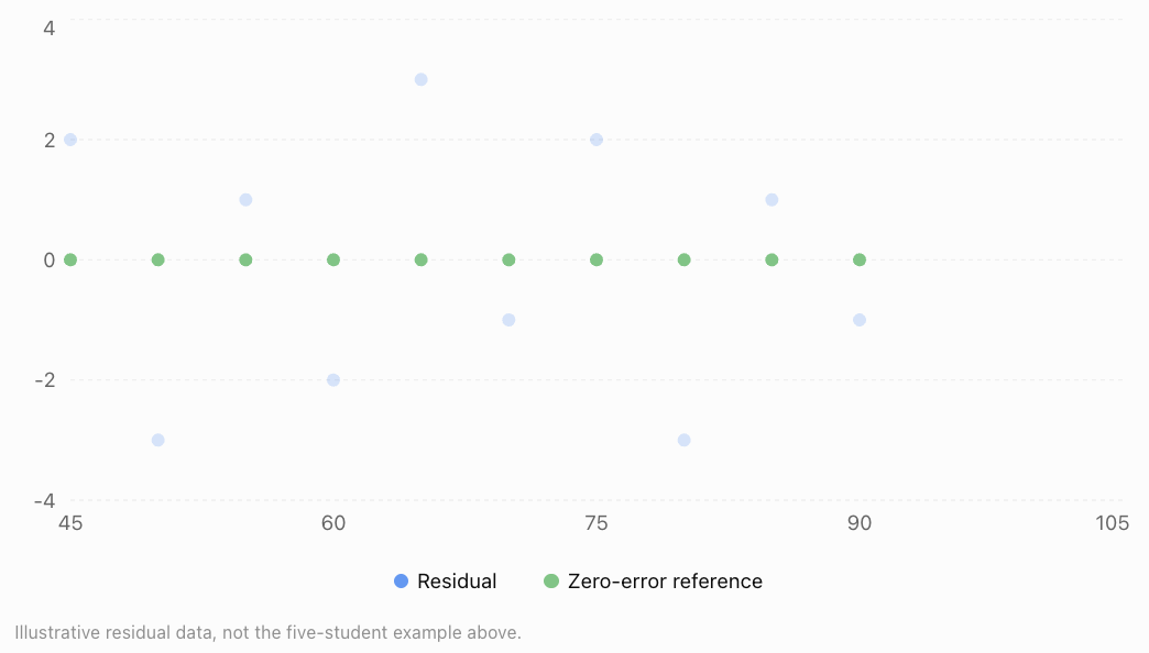
Residual patterns may reveal:
-
Curvature, suggesting that a linear model is inappropriate.
-
Increasing spread, suggesting nonconstant error variance.
-
Unusually large residuals, indicating possible outliers.
-
Clusters or trends, suggesting missing explanatory variables or other model problems.
A residual plot is useful, but it cannot prove that every model assumption is satisfied.
Multicollinearity
Multicollinearity occurs when two or more explanatory variables in a regression model are strongly linearly related.
For example, suppose a model predicts house prices using both floor area in square metres and floor area in square feet.
These variables contain essentially the same information.
This creates perfect multicollinearity, making it impossible to estimate separate coefficients for both variables in an ordinary multiple regression model.
Less extreme multicollinearity can also occur.
For example, study hours and attendance may be strongly correlated.
This can make individual coefficient estimates unstable and difficult to interpret.
Possible solutions
Researchers may:
-
Remove redundant explanatory variables.
-
Combine related variables into a meaningful index.
-
Collect additional observations with more varied combinations of predictors.
-
Use methods such as ridge regression when appropriate.
Multicollinearity is especially problematic when interpreting individual coefficients. It does not always make predictions poor.
Interaction Effects in Statistical Models
Sometimes one variable changes the relationship between another variable and the response.
This is called an interaction.
Suppose examination performance depends on both study time and access to tutoring.
A model might be:
Where:
-
x₁ = study hours
-
x₂ = tutoring status (0 = no tutoring, 1 = tutoring)
-
x₁x₂ = interaction term
Worked Example: Interpreting an Interaction
For a student without tutoring:
x₂ = 0
For a student with tutoring:
x₂ = 1
Simplifying:
The model predicts:
-
Without tutoring, each additional study hour is associated with a 5-point increase.
-
With tutoring, each additional study hour is associated with a 7-point increase.
This suggests that the relationship between study time and examination performance differs depending on tutoring status.
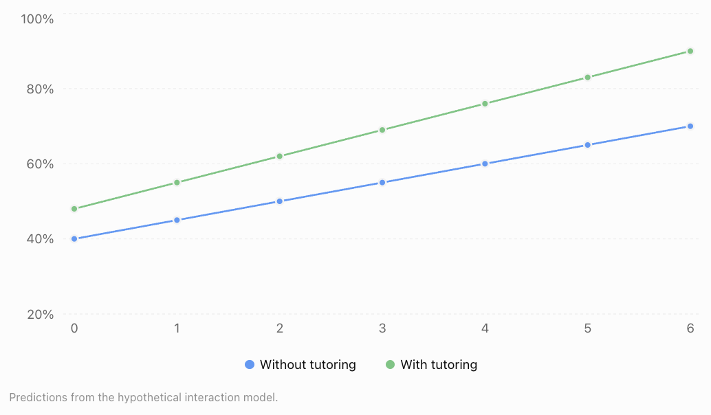
The different slopes indicate an interaction effect.
However, this hypothetical model does not establish that tutoring causes the improvement.
Choosing an Appropriate Statistical Model
Different statistical models are suitable for different types of data.
|
Situation |
Possible statistical model |
|---|---|
|
Predicting a numerical outcome from several variables |
Multiple linear regression |
|
Predicting a yes/no outcome |
Logistic regression |
|
Modelling curved relationships |
Polynomial regression or other nonlinear models |
|
Predicting counts of events |
Poisson regression |
|
Investigating time-dependent data |
Time-series models |
|
Examining repeated observations from the same individuals |
Mixed-effects models |
The choice depends on the response variable, data structure, research question, and assumptions.
Questions to ask when evaluating a model
-
Is the model suitable for the type of response variable?
-
Are the explanatory variables relevant?
-
Have important confounding variables been considered?
-
Are there strong relationships among explanatory variables?
-
Are the model assumptions reasonable?
-
Are the predictions accurate on data not used to fit the model?
-
Is the model being used within a sensible range of values?
A statistically complex model is not automatically more useful than a simpler one.
Communicating Statistical Reasoning
Statistical conclusions should be clear, accurate, and supported by evidence.
A strong statistical explanation includes the following elements.
Research question
State what the investigation is trying to determine.
Example:
"How are study time, attendance, and sleep duration associated with examination scores?"
Methods
Explain how the data were collected and analysed.
Example:
"Data from 150 students were analysed using multiple linear regression."
Results
Report relevant numerical evidence.
Example:
"The model explained 78% of the variation in examination scores in the sample (R² = 0.78)."
Interpretation
Explain what the results mean.
Example:
"After adjusting for attendance and sleep duration, study time remained positively associated with examination performance."
Limitations
Identify reasons for caution.
Example:
"The study was observational, so the results do not establish that increasing study time will cause higher examination scores. Previous achievement and motivation were not measured."
Conclusion
Provide a balanced statement that answers the original research question.
Example:
"Study time, attendance, and sleep duration were useful predictors of examination performance in this sample. Further investigation would be needed to establish causal relationships."
Avoiding misleading language
Compare the following statements.
Misleading: "Studying longer causes higher examination scores."
Better: "Students who studied longer tended to achieve higher examination scores, after accounting for the other variables included in the model."
The second statement is more appropriate when the evidence comes from an observational study.
Real-World Applications
Agriculture
Researchers investigate how sunlight, rainfall, temperature, fertiliser, and soil quality relate to crop yields. Multivariable models can help identify growing conditions associated with better harvests.
Economics and Property
Property prices can be modelled using floor area, location, age, accessibility, and nearby amenities. Analysts must consider how these predictors relate to one another.
Transport Planning
Traffic congestion can be analysed using vehicle numbers, road capacity, weather, public transport availability, and time of day.
Environmental Science
Scientists study relationships between pollution, rainfall, land use, industrial activity, and water quality to understand environmental changes.
Common Mistakes
Mistake 1: Assuming correlation proves causation
Two variables may be associated because of confounding, reverse causation, or other explanations.
Correction: Use language such as "associated with" unless the evidence supports a causal conclusion.
Mistake 2: Ignoring confounding variables
A relationship between two variables may change after accounting for a third variable.
Correction: Consider other factors that may influence both the explanatory variable and the response.
Mistake 3: Interpreting regression coefficients without considering other predictors
In multiple regression, a coefficient represents an adjusted relationship, not simply the overall pairwise association.
Correction: Interpret each coefficient while holding the other included variables constant.
Mistake 4: Assuming a higher R² always means a better model
Adding variables usually increases or preserves training R², even if the additional variables are not useful.
Correction: Consider adjusted R², residuals, and prediction performance on new data.
Mistake 5: Ignoring multicollinearity
Strong relationships among explanatory variables can make individual coefficients unstable.
Correction: Investigate redundant variables and interpret coefficients cautiously.
Mistake 6: Extrapolating beyond the observed data
A model fitted using students who study between one and six hours may produce unrealistic predictions for someone studying twenty hours.
Correction: Make predictions within the range and conditions supported by the data.
Mistake 7: Reporting statistical results without limitations
A model may work well for one dataset but poorly for another population.
Correction: Explain the sample, assumptions, uncertainty, and limitations of the conclusions.
Key Terms
-
Multiple Variable Analysis: Statistical investigation involving several variables simultaneously.
-
Response Variable: The outcome being explained or predicted.
-
Explanatory Variable: A variable used to explain or predict a response.
-
Confounding Variable: A variable associated with both the explanatory variable and the outcome that can distort their apparent relationship.
-
Correlation: A measure of the direction and strength of a relationship between variables.
-
Correlation Matrix: A table displaying pairwise correlation coefficients.
-
Multiple Linear Regression: A method for modelling a numerical response using two or more explanatory variables.
-
Regression Coefficient: A numerical value describing an estimated relationship between a predictor and the response.
-
Residual: The difference between an observed value and a predicted value.
-
R²: The coefficient of determination, measuring the proportion of variation explained by a regression model under the usual least-squares definition.
-
Adjusted R²: A version of R² that accounts for the number of explanatory variables.
-
RMSE: Root Mean Squared Error, a measure of prediction error.
-
Multicollinearity: Strong linear relationships among explanatory variables.
-
Interaction Effect: A situation where the relationship between one predictor and the response depends on another predictor.
-
Statistical Model: A mathematical representation of relationships or patterns in data.
-
Causation: A relationship in which changing one factor produces a change in another.
-
Extrapolation: Using a model to predict outside the range of the observed data.
-
Overfitting: When a model captures random features of training data rather than patterns that generalise well.
Key Takeaways
-
Real-world outcomes are often related to several variables simultaneously.
-
Multiple variable analysis helps researchers investigate these relationships more completely.
-
Confounding variables can create or distort apparent associations.
-
Correlation matrices describe pairwise relationships but do not fully account for other variables.
-
Multiple regression models estimate relationships between an outcome and several predictors.
-
Regression coefficients must be interpreted while holding other included variables constant.
-
Interaction effects occur when the relationship between one variable and the outcome depends on another variable.
-
Statistical models should be evaluated using appropriate measures of fit, prediction errors, assumptions, and residuals.
-
Multicollinearity can make individual regression coefficients difficult to interpret.
-
Strong statistical reasoning includes evidence, appropriate conclusions, and clear discussion of limitations.
Check Your Understanding
Try the following questions before examining the worked answers.
Questions
Question 1: Identifying Variables
A researcher investigates how exercise duration, sleep, and age are related to resting heart rate.
Identify the response variable and three explanatory variables.
Question 2: Confounding Variables
A study finds that people who own more books tend to achieve higher examination scores.
Identify a possible confounding variable and explain why it might influence the relationship.
Question 3: Interpreting Correlation
A dataset gives the following correlations with examination score:
-
Study hours: r = 0.82
-
Sleep duration: r = 0.35
-
Absences: r = −0.71
Which variable has the strongest linear association with examination score? Which relationship is negative?
Question 4: Multiple Regression
A model predicts examination scores using:
Where:
-
x₁ = study hours
-
x₂ = sleep hours
Calculate the predicted score for a student who studies for 5 hours and sleeps for 8 hours.
Question 5: Interpreting Coefficients
Using the model in Question 4, explain the meaning of the coefficient 6.
Question 6: Residuals
A statistical model predicts a score of 78, but the actual score is 72.
Calculate the residual and explain what it means.
Question 7: Comparing Models
Two models produce these results on the same test dataset.
|
Measure |
Model A |
Model B |
|---|---|---|
|
Test R² |
0.68 |
0.81 |
|
Test RMSE |
8.5 |
6.1 |
Which model performs better on the test dataset? Explain.
Question 8: Multicollinearity
A house-price model includes floor area measured in square metres and floor area measured in square feet.
Explain why this creates a problem.
Question 9: Interaction Effects
A model is:
Where x₂ is either 0 or 1.
Determine the relationship between ŷ and x₁ when x₂ = 0 and when x₂ = 1.
Question 10: Statistical Communication
A researcher finds that students who exercise more frequently tend to achieve higher examination scores.
Explain why the statement "Exercise causes higher examination scores" may be misleading. Write a more appropriate conclusion.
Fully Worked Answers
Answer 1: Identifying Variables
The response variable is resting heart rate, because it is the outcome being investigated.
The explanatory variables are exercise duration, sleep duration, and age.
These variables may help explain variation in resting heart rate.
Answer 2: Confounding Variables
A possible confounding variable is family socioeconomic background.
Families with greater financial resources may be able to purchase more books and provide additional educational opportunities.
This could influence both book ownership and examination performance.
Therefore, the relationship between book ownership and examination scores does not necessarily mean that owning more books causes higher scores.
Answer 3: Interpreting Correlation
Compare the absolute values of the correlation coefficients.
-
Study hours: |0.82| = 0.82
-
Sleep duration: |0.35| = 0.35
-
Absences: |−0.71| = 0.71
The strongest linear association is between study hours and examination score, because 0.82 has the greatest absolute value.
Absences have a negative correlation with examination scores.
This means students with more absences tend to have lower examination scores.
Answer 4: Multiple Regression
Given:
Substitute x₁ = 5 and x₂ = 8.
The predicted examination score is 74%.
Answer 5: Interpreting Coefficients
The coefficient 6 represents the estimated change in examination score associated with one additional hour of study, holding sleep duration constant.
Therefore, the model predicts a 6-percentage-point increase in examination score for each additional study hour, assuming the linear model is appropriate.
This does not necessarily imply that increasing study time causes the score to rise by six points.
Answer 6: Residuals
Residual = Actual − Predicted
Residual = 72 − 78
The residual is −6.
This means the model overestimated the student's examination score by 6 percentage points.
Answer 7: Comparing Models
Model B has:
-
A higher test R² (0.81 compared with 0.68).
-
A lower test RMSE (6.1 compared with 8.5).
Therefore, Model B performs better on the test dataset according to both measures.
However, we would still examine whether its assumptions are reasonable and whether its performance generalises to other students.
Answer 8: Multicollinearity
Floor area in square metres and floor area in square feet represent exactly the same physical quantity.
Their relationship is:
Area in square feet ≈ 10.764 × Area in square metres
Therefore, the two explanatory variables are perfectly linearly related.
This creates perfect multicollinearity, so an ordinary multiple regression model cannot uniquely estimate separate coefficients for both.
A sensible solution is to use only one floor-area measurement.
Answer 9: Interaction Effects
The model is:
When x₂ = 0:
The slope with respect to x₁ is 4.
When x₂ = 1:
The slope with respect to x₁ is 7.
Therefore, the relationship between x₁ and the predicted outcome differs according to the value of x₂.
This is an interaction effect.
Answer 10: Statistical Communication
The original statement is misleading because an association does not necessarily demonstrate causation.
Other factors, such as sleep, motivation, family resources, or general health, might influence both exercise habits and academic performance.
A more appropriate conclusion is:
"Students who exercised more frequently tended to achieve higher examination scores in the observed sample. However, the study does not establish that exercise directly caused the higher scores."
This conclusion accurately describes the evidence while acknowledging its limitations.
Final Reflection
Multiple variable analysis is an essential part of modern statistics because most real-world situations involve several connected factors.
A useful statistical investigation does more than identify patterns. It considers possible confounding variables, interprets the contributions of multiple predictors, evaluates model performance, and communicates conclusions without overstating what the evidence demonstrates.
The central principle is that statistical relationships must be interpreted in context. A strong model is not simply one that fits the data well, but one that produces meaningful, reliable, and appropriately qualified conclusions.