Introduction

Imagine that a school wants to investigate whether the number of hours students spend studying can help predict their examination scores. After collecting data, the school notices that students who study longer generally achieve higher scores. However, the points on a scatter plot do not form a perfectly straight line.

How can we describe this relationship mathematically? How can we use it to predict examination results? And how can we determine whether our predictions are reliable?

Linear regression provides a method for answering these questions.

Linear regression is a statistical technique that models the relationship between a numerical explanatory variable and a numerical response variable using a straight line. It allows us to identify trends, make predictions, measure prediction errors, and evaluate how well a mathematical model represents real data.

Linear regression is widely used in science, economics, engineering, medicine, environmental research, and business.

What Is Linear Regression?

Linear regression is a method of finding a straight line that best describes the relationship between two quantitative variables.

This line is called the regression line, or line of best fit.

A scatter plot displays the original observations, while the regression line summarises their overall linear trend.

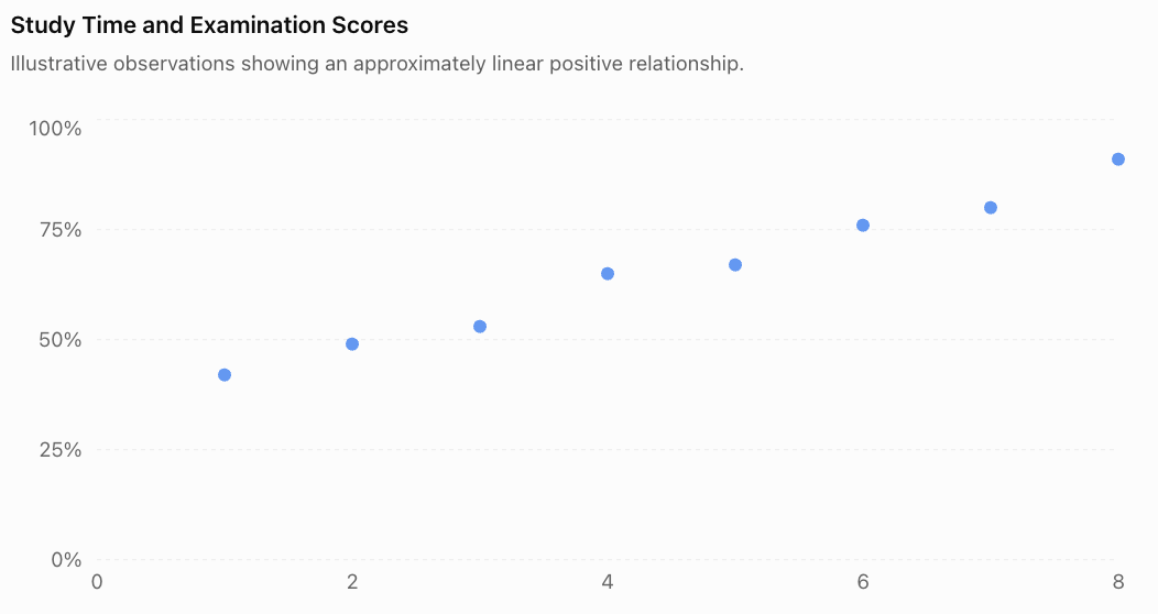
The points generally rise from left to right, indicating a positive linear association.

A regression line allows us to represent this trend with an equation rather than simply describing it visually.

The Regression Equation

A simple linear regression equation is commonly written as:

Where:

• ŷ (y-hat) = predicted value of the response variable

• x = explanatory or predictor variable

• a = y-intercept of the regression line

• b = slope or regression coefficient

The symbol ŷ is used instead of y because the regression equation produces a prediction, which may differ from the observed value.

Understanding the Slope

The slope, b, describes how much the predicted response changes for each one-unit increase in x.

• If b is positive, the predicted response increases as x increases.

• If b is negative, the predicted response decreases as x increases.

• If b is zero, the model predicts the same response regardless of x.

Understanding the Intercept

The intercept, a, is the predicted response when x = 0.

However, the intercept is not always meaningful in a real-world context. If zero lies outside the observed range, interpreting the intercept may involve unreliable extrapolation.

Determining a Line of Best Fit

A line of best fit can be estimated visually or calculated mathematically.

Method 1: Drawing a Line of Best Fit by Eye

When using a scatter plot:

1. Plot all paired observations accurately.

2. Identify the overall direction of the points.

3. Draw a straight line through the centre of the pattern.

4. Try to balance the points above and below the line.

5. Choose two well-separated points on the line to estimate its slope and intercept.

A visually estimated line is useful for understanding trends, but different people may draw slightly different lines.

For precise statistical analysis, we use the least-squares method.

Method 2: The Least-Squares Regression Line

The least-squares method finds the line that minimises the sum of the squared vertical differences between observed and predicted values.

These vertical differences are called residuals.

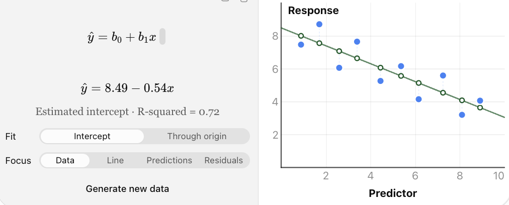
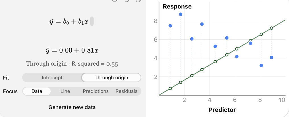
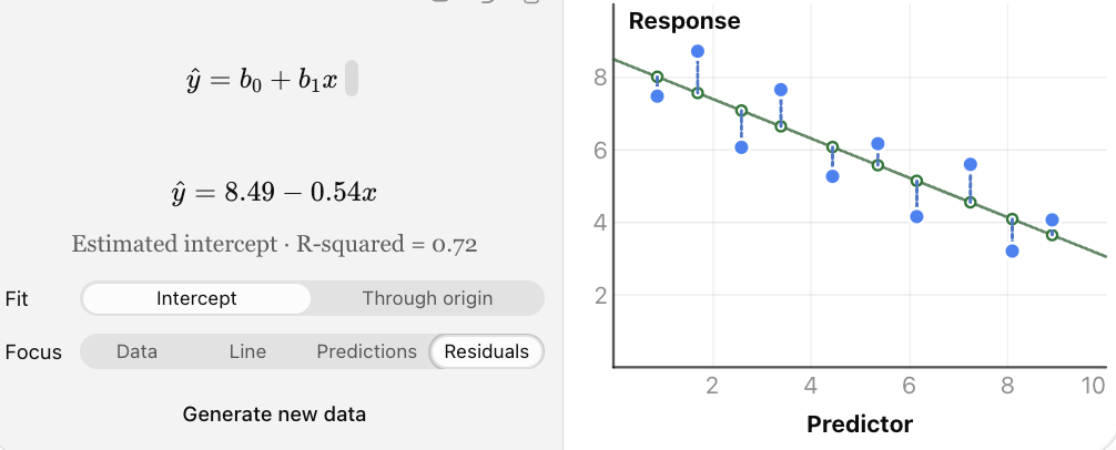
Interactive regression model: move the observed points to see how the least-squares line changes. The vertical gaps between points and the fitted line represent residuals.

Why square the residuals?

Squaring ensures that positive and negative errors do not cancel each other. It also gives greater weight to large errors.

The quantity minimised is called the sum of squared errors, or SSE:

The least-squares line has the smallest possible SSE among straight lines with an intercept fitted to the same dataset.

Calculating the Least-Squares Regression Line

For simple linear regression, the slope is:

The intercept is:

Where:

• n = number of paired observations

• Σxy = sum of products of corresponding x- and y-values

• Σx = sum of x-values

• Σy = sum of y-values

• Σx² = sum of squared x-values

• x̄ = mean of x-values

• ȳ = mean of y-values

The slope formula requires variation in x; if all x-values are identical, the usual least-squares slope cannot be calculated.

Worked Example 1: Finding a Regression Equation

A teacher records the number of hours five students spend studying and their scores on a short assessment.

Determine the least-squares regression equation.

Step 1: Construct a calculation table.

Therefore:

n = 5

Σx = 15

Σy = 20

Σx² = 55

Σxy = 69

Step 2: Calculate the slope.

Step 3: Calculate the means.

Step 4: Calculate the intercept.

Step 5: Write the regression equation.

This equation represents the least-squares line of best fit.

Interpreting the Equation

The slope of 0.9 means that each additional hour of study is associated with an increase of 0.9 points in the predicted assessment score.

The intercept of 1.3 means that the model predicts a score of 1.3 points when study time is zero hours.

Because zero hours is outside the observed study-time range of 1–5 hours, the intercept should be interpreted cautiously.

Making Predictions Using Regression

Once a regression equation has been determined, it can be used to estimate the response variable for a particular explanatory-variable value.

Worked Example 2: Predicting an Assessment Score

Using the regression equation:

ŷ = 1.3 + 0.9x

Predict the assessment score for a student who studies for 4 hours.

Step 1: Substitute x = 4.

ŷ = 1.3 + 0.9(4)

Step 2: Simplify.

ŷ = 1.3 + 3.6

The predicted score is 4.9 points.

The actual score of the student who studied for 4 hours was 4 points, illustrating that a regression prediction does not necessarily match an observation exactly.

Worked Example 3: Predicting House Prices

Suppose a property analyst develops the model:

ŷ = 80,000 + 2,500x

Where:

• x = floor area in square metres

• ŷ = predicted house price in dollars

Predict the price of a house with a floor area of 120 m².

ŷ = 80,000 + 2,500(120)

ŷ = 80,000 + 300,000

The model predicts a price of $380,000.

The slope indicates an additional $2,500 in predicted price per square metre of floor area.

This does not mean that increasing a particular house's area by one square metre would necessarily cause its price to rise by exactly $2,500. Other factors, such as location and condition, also matter.

Interpolation and Extrapolation

Regression predictions are not equally reliable for all values of x.

Interpolation

Interpolation occurs when a prediction is made within the range of x-values used to develop the model.

For example, if study times range from 1 to 8 hours, predicting a score for 5 hours is interpolation.

Extrapolation

Extrapolation occurs when a prediction is made outside the observed range.

Predicting the score for a student who studies for 20 hours would be extrapolation.

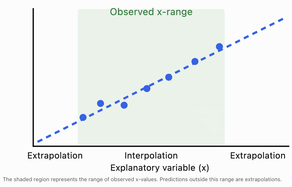
Extrapolation is often less reliable because the relationship may change outside the observed range.

For example, a model relating study time to examination score cannot reasonably predict examination scores greater than 100% indefinitely.

Understanding Residuals

A regression line does not usually pass through every observation.

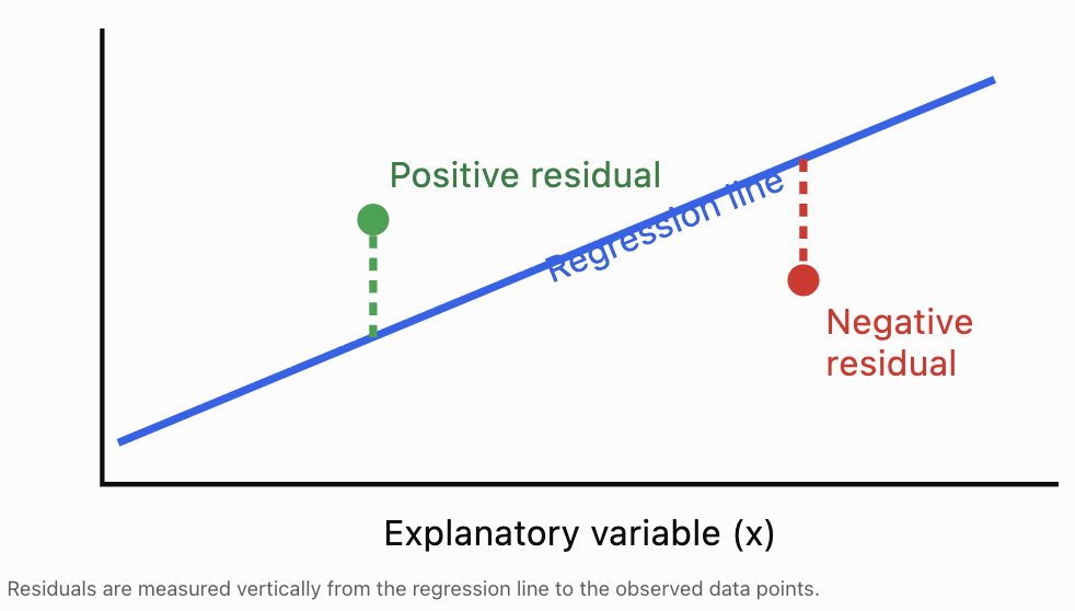
The difference between an observed value and its predicted value is called a residual.

The residual formula is:

Where:

• e = residual

• y = observed value

• ŷ = predicted value

A residual measures the prediction error for one observation.

Interpreting Residual Signs

• Positive residual: The observed value is greater than predicted; the point lies above the regression line.

• Negative residual: The observed value is less than predicted; the point lies below the regression line.

• Zero residual: The observed value equals the predicted value; the point lies on the regression line.

  

  Worked Example 4: Calculating Residuals

  Use the regression equation from Worked Example 1:

  ŷ = 1.3 + 0.9x

  Calculate the predicted values and residuals for all five students.

  x	Observed y	Predicted ŷ	Residual (y − ŷ)
  1	2	2.2	−0.2
  2	3	3.1	−0.1
  3	5	4.0	+1.0
  4	4	4.9	−0.9
  5	6	5.8	+0.2

  For the third student:

  e = 5 − 4.0 = +1.0

  The actual score was 1 point higher than predicted.

  For the fourth student:

  e = 4 − 4.9 = −0.9

  The actual score was 0.9 points lower than predicted.

  For an ordinary least-squares regression with an intercept, the residuals sum to zero, apart from rounding.

  Here:

  −0.2 − 0.1 + 1.0 − 0.9 + 0.2 = 0

  This property does not mean the predictions are perfect; positive and negative residuals can cancel.

   

  Residual Plots

  A residual plot displays residuals on the vertical axis and the explanatory variable (or fitted values) on the horizontal axis.

  Residual plots are useful for checking whether a linear model is appropriate.

  For the five-student example:

  

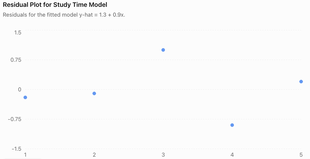
  The residuals appear on both sides of zero without a clear curved trend. This is consistent with a linear model, although five observations are too few to assess model assumptions confidently.

  Recognising Residual Patterns

  

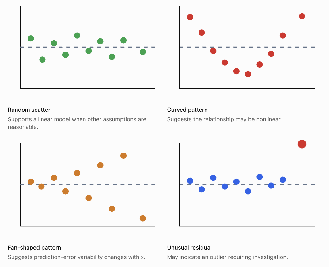
  A good residual plot should generally show points scattered around zero without an obvious systematic pattern.

  A curved pattern suggests that a straight line may not adequately describe the relationship.

  A fan-shaped pattern suggests heteroscedasticity, meaning that the variability of errors changes across the predictor range.

  Residual plots can also help identify unusual observations, although additional diagnostics may be needed.

   

  Evaluating Model Accuracy

  Finding a regression equation is only the beginning. We must also determine how accurately the model describes the data and how useful its predictions are.

  Several statistical measures help us evaluate model performance.

  Sum of Squared Errors (SSE)

  SSE measures the total squared prediction error:

  \[ SSE=\sum (y-\hat y)^2 \]

  Smaller SSE values indicate a closer fit for models evaluated on the same observations and response scale.

  Using the five-student dataset:

  Residual	Residual²
  −0.2	0.04
  −0.1	0.01
  +1.0	1.00
  −0.9	0.81
  +0.2	0.04
  Total	1.90

  Therefore:

  \[ \boxed{SSE=1.90} \]

  Mean Squared Error (MSE)

  MSE is the average squared prediction error.

  For descriptive or predictive evaluation of n observations:

  \[ MSE=\frac{SSE}{n} \]

  For our dataset:

  \[ MSE=\frac{1.90}{5}=\boxed{0.38} \]

  Smaller MSE values generally indicate better predictions on comparable data.

  In statistical inference, a related estimate of residual error variance uses SSE/(n − 2) for simple linear regression with an intercept. This accounts for the two fitted parameters.

  Root Mean Squared Error (RMSE)

  RMSE is the square root of MSE.

  \[ RMSE=\sqrt{\frac{SSE}{n}} \]

  For the five-student dataset:

  \[ RMSE=\sqrt{0.38} \]

  \[ \boxed{RMSE\approx0.616} \]

  The RMSE is approximately 0.616 assessment points.

  Unlike MSE, RMSE is expressed in the same units as the response variable, making it easier to interpret.

  Mean Absolute Error (MAE)

  MAE measures the average absolute prediction error.

  \[ MAE=\frac{\sum |y-\hat y|}{n} \]

  For our dataset:

  \[ MAE=\frac{0.2+0.1+1.0+0.9+0.2}{5} \]

  \[ MAE=\frac{2.4}{5}=\boxed{0.48} \]

  The average absolute prediction error is 0.48 points.

  Unlike MSE and RMSE, MAE does not square errors, so it is less sensitive to a small number of very large errors.

   

  The Coefficient of Determination: R²

  The coefficient of determination, written R², describes the proportion of variation in the response variable explained by the fitted regression model relative to a model that always predicts the sample mean.

  For ordinary least-squares regression with an intercept:

  \[ R^2=1-\frac{SSE}{SST} \]

  Where:

  • SSE = sum of squared residuals

  • SST = total sum of squares

  • SST = Σ(y − ȳ)²

  For simple linear regression with an intercept, R² is also equal to the square of the Pearson correlation coefficient.

  \[ R^2=r^2 \]

  Worked Example 5: Calculating R²

  For our five-student dataset:

  y-values: 2, 3, 5, 4, 6

  Mean score:

  ȳ = 4

  Calculate SST:

  SST = (2 − 4)² + (3 − 4)² + (5 − 4)² + (4 − 4)² + (6 − 4)²

  SST = 4 + 1 + 1 + 0 + 4

  SST = 10

  We previously calculated SSE = 1.90.

  Therefore:

  \[ R^2=1-\frac{1.90}{10} \]

  \[ \boxed{R^2=0.81} \]

  The model accounts for 81% of the variation in assessment scores within this dataset, relative to predicting the mean score.

  The remaining 19% is not explained by the fitted line.

  This does not mean that study time causes exactly 81% of examination performance. R² measures model fit, not causation.

  

  Interpreting R² Carefully

  A high R² indicates that the fitted model explains a large proportion of the observed variation.

  However, a high R² does not guarantee that:

  • The relationship is causal.

  • The model is appropriate for every situation.

  • The model will predict new observations accurately.

  • There are no influential outliers.

  • The model's assumptions are satisfied.

  Similarly, a low R² does not automatically make a model useless. In fields involving highly variable human behaviour, even modest predictive relationships may be informative.

   

  Comparing Measures of Model Accuracy

  Measure	What it measures	Preferred direction
  SSE	Total squared residual error	Lower
  MSE	Average squared prediction error	Lower
  RMSE	Typical error scale, with large errors emphasised	Lower
  MAE	Average absolute prediction error	Lower
  R²	Proportion of sample variation explained by the model	Higher

  These measures should be compared only when appropriate. For example, SSE depends on the number of observations, while MSE and RMSE depend on the scale of the response variable.

  A model should also be tested on data that were not used to fit it.

   

  Training Data and Test Data

  A regression model may fit the observations used to construct it very well but perform poorly on new data.

  This is called overfitting when the model captures patterns or noise that do not generalise.

  To evaluate predictive performance, statisticians often divide data into:

  • Training data: Used to calculate the regression equation.

  • Test data: Used to evaluate predictions on observations not used to fit the model.

  For smaller datasets, cross-validation may provide a more informative assessment than a single train–test split.

  Worked Example 6: Comparing Two Models

  Two regression models are evaluated on the same unseen test dataset.

  Measure	Model A	Model B
  Training RMSE	2.1	1.2
  Test RMSE	2.4	5.8
  Training R²	0.88	0.97

  Model B fits the training data more closely, but Model A makes substantially smaller errors on the test data.

  Therefore, Model A is the better predictive choice based on these test results.

  Model B may have overfitted the training observations.

  This example illustrates why model evaluation should not rely only on training accuracy.

   

  Assumptions of Linear Regression

  Linear regression is most reliable when its underlying assumptions are reasonably satisfied.

  Linearity

  The mean response should have an approximately linear relationship with the explanatory variable.

  A curved residual pattern suggests that a linear model may be inappropriate.

  Independence

  Observations or model errors should be independent where required by the study design.

  For example, measurements collected repeatedly from the same person may be related and require specialised methods.

  Constant Error Variance

  The spread of errors should remain approximately constant across fitted values for standard regression inference.

  A fan-shaped residual plot may indicate that this assumption is violated.

  Approximately Normal Errors for Certain Inference Procedures

  Normality of errors is particularly relevant for exact small-sample confidence intervals and hypothesis tests.

  Normality is not required simply to calculate the least-squares line.

  Absence of Highly Influential Observations

  An extreme observation can substantially change the slope and intercept.

  Researchers should investigate unusual observations rather than automatically deleting them.

  Other Important Considerations

  Even if these assumptions are reasonably satisfied, omitted variables, measurement errors, biased sampling, or inappropriate extrapolation can limit a model's usefulness.

   

  Using Technology for Linear Regression

  Regression calculations can be performed using spreadsheets, graphing calculators, and statistical software.

  In Excel or Google Sheets, suppose the x-values are in A2:A11 and y-values are in B2:B11.

  Purpose	Formula
  Calculate slope	=SLOPE(B2:B11,A2:A11)
  Calculate intercept	=INTERCEPT(B2:B11,A2:A11)
  Calculate R²	=RSQ(B2:B11,A2:A11)
  Calculate Pearson's r	=CORREL(A2:A11,B2:B11)

  To make a prediction, use:

  =INTERCEPT(B2:B11,A2:A11)+SLOPE(B2:B11,A2:A11)*D2

  Where D2 contains the x-value for which a prediction is required.

  For a visual approach, create a scatter plot and add a linear trendline, selecting the options to display the equation and R² value.

  Remember that spreadsheet software may round the displayed equation. Calculations using full-precision coefficients are generally more accurate.

   

  Real-World Applications of Linear Regression

  FRANCE-RESEARCH-CLIMATE

   

   

   

  Climate and Environmental Science

  Researchers use regression to investigate temperature trends, rainfall patterns, pollution concentrations, and environmental changes over time.

   

  Intelligent Infrastructure Laboratory | ICAIR

   

   

   

  Engineering

  Engineers model relationships between applied force and deformation, electrical current and voltage, or material properties and performance.

   

  Become a Financial Analyst After Completing Your Online BCom

   

   

   

  Business and Economics

  Analysts use regression to predict sales, examine relationships between advertising and revenue, and estimate how prices vary with product characteristics.

   

  Clinical Research Course Certificate | Free & Fast Course

   

   

   

  Medicine and Health Research

  Researchers investigate relationships between age, physical measurements, exercise, and health outcomes. Regression helps quantify associations while accounting for uncertainty.

   

  Common Mistakes

  Common mistake	Correction
  Assuming a regression line passes through every observation	The line minimises total squared residuals; individual residuals are usually nonzero.
  Confusing observed y with predicted ŷ	Use y for actual measurements and ŷ for predictions.
  Calculating residuals as ŷ − y	Residual = observed − predicted.
  Interpreting the intercept without considering context	The intercept may be meaningless if x = 0 is outside the observed range.
  Assuming a high R² proves causation	R² describes model fit, not cause and effect.
  Ignoring residual patterns	Curved or fan-shaped patterns can reveal model problems.
  Extrapolating far beyond the data	The relationship may change outside the observed range.
  Comparing SSE values from different-sized datasets without caution	SSE depends on sample size and response scale.
  Assuming low training error guarantees accurate predictions	Evaluate the model on unseen data.
  Automatically removing outliers	Investigate unusual observations and their influence before deciding how to handle them.

   

  Key Terms

  • Linear regression: A statistical method that models a relationship between numerical variables using a straight line.

  • Regression line: A fitted line used to summarise a linear relationship and make predictions.

  • Line of best fit: A line that represents the overall trend in a scatter plot.

  • Least-squares method: A method that minimises the sum of squared residuals.

  • Explanatory variable: A variable used to predict or explain another variable.

  • Response variable: The variable being predicted or studied.

  • Predicted value (ŷ): The response value calculated using the regression equation.

  • Regression coefficient: A parameter of a regression model, such as its slope.

  • Slope: The predicted change in y for a one-unit increase in x.

  • Intercept: The predicted y-value when x = 0.

  • Residual: The difference between an observed and predicted value.

  • Residual plot: A graph used to investigate patterns in regression errors.

  • SSE: Sum of squared errors.

  • MSE: Mean squared error.

  • RMSE: Root mean squared error.

  • MAE: Mean absolute error.

  • R²: Coefficient of determination; a measure of the proportion of variation explained by the fitted model.

  • Interpolation: Prediction within the observed range.

  • Extrapolation: Prediction beyond the observed range.

  • Heteroscedasticity: Unequal error variance across the predictor or fitted-value range.

  • Overfitting: Fitting a model too closely to training data in a way that harms generalisation.

  • Cross-validation: A method for evaluating predictive performance using repeated training and validation partitions.

  • Influential observation: An observation that substantially affects the fitted model.

   

  Key Takeaways

  1. Linear regression models the relationship between an explanatory variable and a response variable using a straight line.

  2. The least-squares method finds the line that minimises the sum of squared residuals.

  3. The slope describes the predicted change in the response for a one-unit increase in the explanatory variable.

  4. The intercept represents the predicted response when the explanatory variable is zero, although it may not always be meaningful.

  5. Regression equations allow us to make predictions, but extrapolation is less reliable than interpolation.

  6. A residual is the difference between an observed value and its predicted value.

  7. Residual plots help identify nonlinearity, unequal error variance, and unusual observations.

  8. SSE, MSE, RMSE, MAE, and R² provide different ways of evaluating model performance.

  9. A high R² does not prove causation or guarantee accurate future predictions.

  10. Reliable regression analysis requires appropriate assumptions, careful interpretation, and evaluation using new data.

   

  Check Your Understanding

  Question 1: Understanding Regression Equations

  A regression equation is:

  ŷ = 15 + 4x

  Identify the slope and intercept.

  Explain what each represents.

  Question 2: Making Predictions

  A business uses the regression equation:

  ŷ = 120 + 35x

  Where x is advertising expenditure in hundreds of dollars and ŷ is predicted sales revenue in hundreds of dollars.

  Predict the sales revenue when advertising expenditure is $500.

  Question 3: Calculating Residuals

  A regression model predicts a student's score to be 72 points.

  The student actually scores 78 points.

  Calculate the residual and interpret its sign.

  Question 4: Finding a Regression Line

  Use the following data to calculate the least-squares regression equation.

  x	y
  1	3
  2	5
  3	4
  4	8

  Calculate the slope and intercept.

  Question 5: Evaluating R²

  A regression model has R² = 0.64.

  Explain what this means and identify one conclusion that cannot be justified from R² alone.

  Question 6: Interpreting a Residual Plot

  A residual plot shows a clear U-shaped pattern.

  What does this suggest about the regression model?

  Question 7: Comparing Models

  Two regression models predict the same response variable on the same test dataset.

  Measure	Model A	Model B
  RMSE	4.2	2.7
  MAE	3.6	2.1

  Which model has better predictive accuracy according to these measures? Explain.

  Question 8: Extrapolation

  A scientist develops a regression model using temperatures between 10°C and 40°C.

  The model is then used to predict a response at 85°C.

  Explain why this prediction may be unreliable.

   

  Fully Worked Answers

  Answer 1

  The equation is:

  ŷ = 15 + 4x

  The slope is 4.

  This means the predicted response increases by 4 units for each one-unit increase in x.

  The intercept is 15.

  This means the predicted response is 15 when x = 0.

  Whether this intercept has practical meaning depends on the context and observed x-range.

  Answer 2

  Advertising expenditure is $500.

  Since x is measured in hundreds of dollars:

  x = 5

  Substitute:

  ŷ = 120 + 35(5)

  ŷ = 120 + 175

  ŷ = 295

  Since revenue is also measured in hundreds of dollars:

  295 × 100 = 29,500

  Predicted sales revenue = $29,500.

  Answer 3

  Residual = observed − predicted

  e = 78 − 72

  \[ \boxed{e=+6} \]

  The positive residual means the student's actual score was 6 points higher than the model predicted.

  Answer 4

  Construct the calculation table.

  x	y	x²	xy
  1	3	1	3
  2	5	4	10
  3	4	9	12
  4	8	16	32
  10	20	30	57

  n = 4

  Calculate the slope:

  \[ b=\frac{4(57)-(10)(20)}{4(30)-10^2} \]

  \[ b=\frac{228-200}{120-100} =\frac{28}{20} \]

  \[ b=1.4 \]

  Calculate the means:

  x̄ = 10/4 = 2.5

  ȳ = 20/4 = 5

  Calculate the intercept:

  a = 5 − 1.4(2.5)

  a = 5 − 3.5

  a = 1.5

  Therefore:

  \[ \boxed{\hat y=1.5+1.4x} \]

  Answer 5

  R² = 0.64 means the fitted model explains 64% of the variation in the observed response variable, relative to predicting its sample mean.

  The remaining 36% is not explained by the model.

  This does not prove that the explanatory variable causes changes in the response variable, nor does it guarantee accurate predictions on new data.

  Answer 6

  A U-shaped residual pattern suggests that the underlying relationship may be nonlinear.

  A straight-line model is systematically overpredicting or underpredicting in different regions.

  A nonlinear model, such as a quadratic regression model, may describe the relationship more appropriately.

  Answer 7

  Model B has the lower RMSE and MAE.

  RMSE:

  • Model A = 4.2

  • Model B = 2.7

  MAE:

  • Model A = 3.6

  • Model B = 2.1

  Both measures favour Model B.

  Therefore, Model B has better predictive accuracy on the given test dataset according to these measures.

  Answer 8

  The prediction at 85°C is extrapolation because 85°C lies outside the observed temperature range of 10°C to 40°C.

  The relationship may not remain linear at higher temperatures.

  The model may therefore produce an inaccurate or unrealistic prediction.

  Additional observations at higher temperatures would be needed to evaluate the relationship more reliably.

   

  Final Reflection

  Linear regression transforms patterns in scatter plots into mathematical models that can be interpreted, tested, and used for predictions.

  However, calculating a line of best fit is only part of a complete statistical investigation. We must also examine residuals, measure prediction errors, check model assumptions, and determine whether predictions are being made within a reasonable range.

  A useful regression model is not simply one that fits existing data closely. It is one that represents the relationship appropriately and makes sufficiently reliable predictions for its intended purpose.