Regression, Correlation, and Statistical Modelling
1. Scatter Plots and Correlation
Learning outcomes
- I can construct scatter plots.
- I can describe correlation strength and direction.
- I can calculate correlation coefficients.
- I can interpret relationships between variables.
- I can distinguish correlation from causation.
Introduction
Many real-world situations involve relationships between two variables. For example, does spending more time studying lead to higher examination scores? Do taller people tend to have larger shoe sizes? Does the price of a car decrease as it gets older?
Statisticians investigate questions like these using scatter plots and correlation.
A scatter plot is a graph that displays pairs of numerical data. By examining the pattern of points, we can identify relationships, estimate their strength, and make predictions.
However, one of the most important principles in statistics is that correlation does not necessarily mean causation. Two variables may be related without one directly causing the other.
Understanding scatter plots and correlation allows us to analyse data, recognise patterns, evaluate evidence, and avoid misleading conclusions.
What Is a Scatter Plot?
A scatter plot, also called a scatter diagram, displays the relationship between two quantitative variables.
Each observation is represented by a point with coordinates (x, y).
-
The horizontal axis (x-axis) usually represents the explanatory or predictor variable.
-
The vertical axis (y-axis) usually represents the response or outcome variable.
-
Each point represents one pair of measurements.
For example, consider the relationship between hours spent studying and examination scores.
|
Study time (hours) |
Examination score (%) |
|---|---|
|
1 |
42 |
|
2 |
48 |
|
3 |
55 |
|
4 |
63 |
|
5 |
68 |
|
6 |
76 |
|
7 |
82 |
|
8 |
89 |
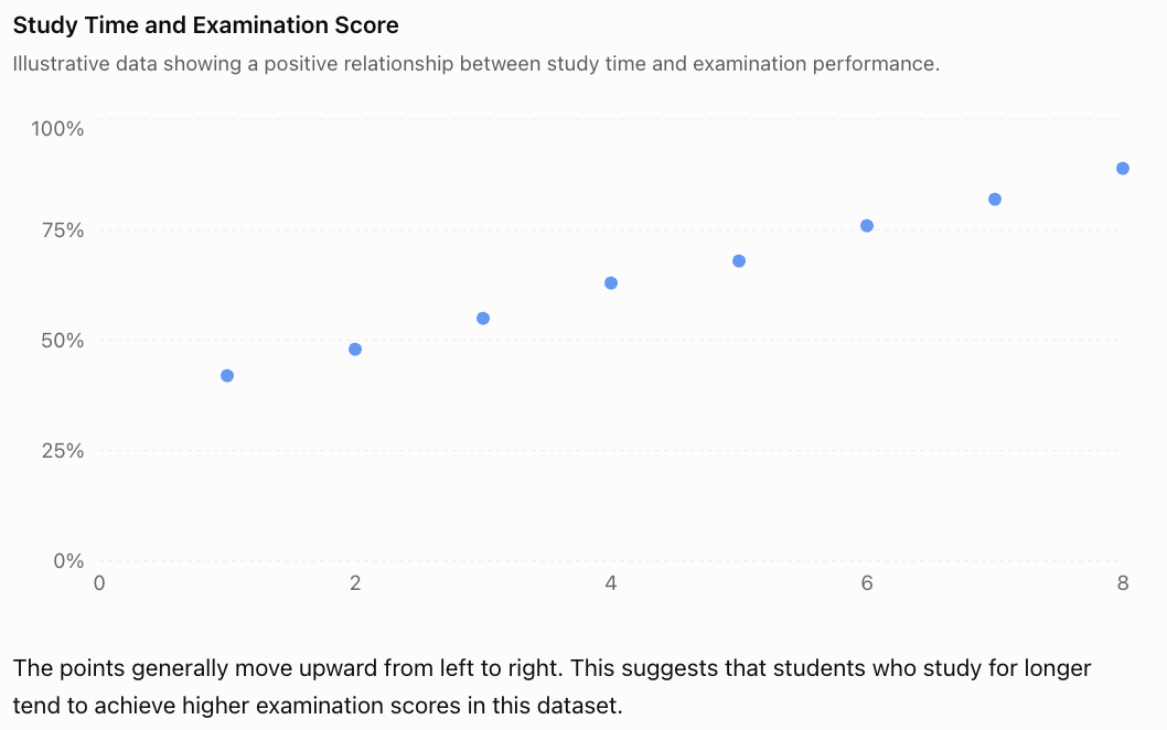
The points generally move upward from left to right. This suggests that students who study for longer tend to achieve higher examination scores in this dataset.
This is an example of positive correlation.
Notice that the graph shows an association. It does not establish that additional study time alone caused the higher scores.
Constructing a Scatter Plot
To construct a scatter plot correctly, follow these steps.
-
Identify the variables. Decide which variable belongs on each axis.
-
Choose suitable scales. Make sure the scales include all the observations and use consistent intervals.
-
Label both axes. Include the variable names and units where appropriate.
-
Plot each coordinate pair. For example, (3, 55) represents 3 hours of study and a score of 55%.
-
Examine the pattern. Look for direction, strength, shape, clusters, and unusual points.
Unlike a line graph showing measurements over time, a scatter plot generally does not connect consecutive points.
Worked Example: Constructing a Scatter Plot
A scientist records the temperature and number of ice creams sold at a shop.
|
Temperature (°C) |
Ice creams sold |
|---|---|
|
20 |
30 |
|
22 |
42 |
|
24 |
50 |
|
26 |
65 |
|
28 |
73 |
|
30 |
88 |
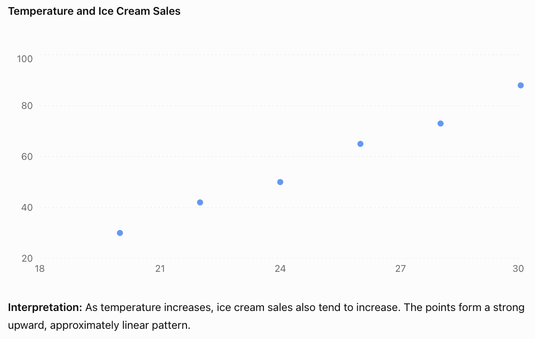
Understanding Correlation
Correlation describes the direction and strength of an association between two variables.
For linear relationships, there are three main directions.
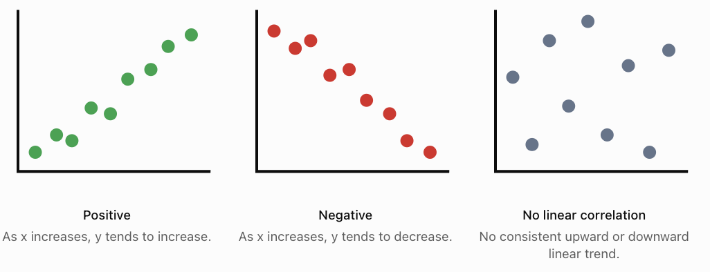
Positive Correlation
Positive correlation occurs when larger values of one variable tend to be associated with larger values of another.
Examples include height and arm span, temperature and ice cream sales, and hours of exercise and calories burned during exercise.
Negative Correlation
Negative correlation occurs when larger values of one variable tend to be associated with smaller values of another.
Examples include vehicle age and resale value, distance remaining and distance travelled along a fixed route, and time spent braking and vehicle speed during a braking event.
No Linear Correlation
Two variables have little or no linear correlation when there is no consistent straight-line trend.
For example, a dataset comparing students' shoe sizes and examination scores might show no meaningful linear association.
Importantly, no linear correlation does not necessarily mean there is no relationship at all. The relationship might be curved.
Strength of Correlation
The strength of linear correlation describes how closely the points follow a straight-line pattern.
-
Strong correlation: Points lie close to a straight line.
-
Moderate correlation: A general trend is visible, but points are more spread out.
-
Weak correlation: Points are widely scattered, with only a slight linear trend.
-
Perfect correlation: Every point lies exactly on a straight line.
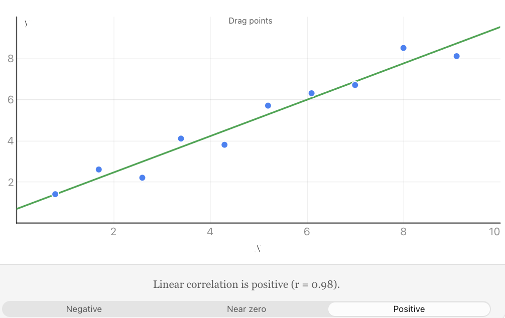
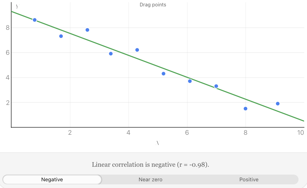
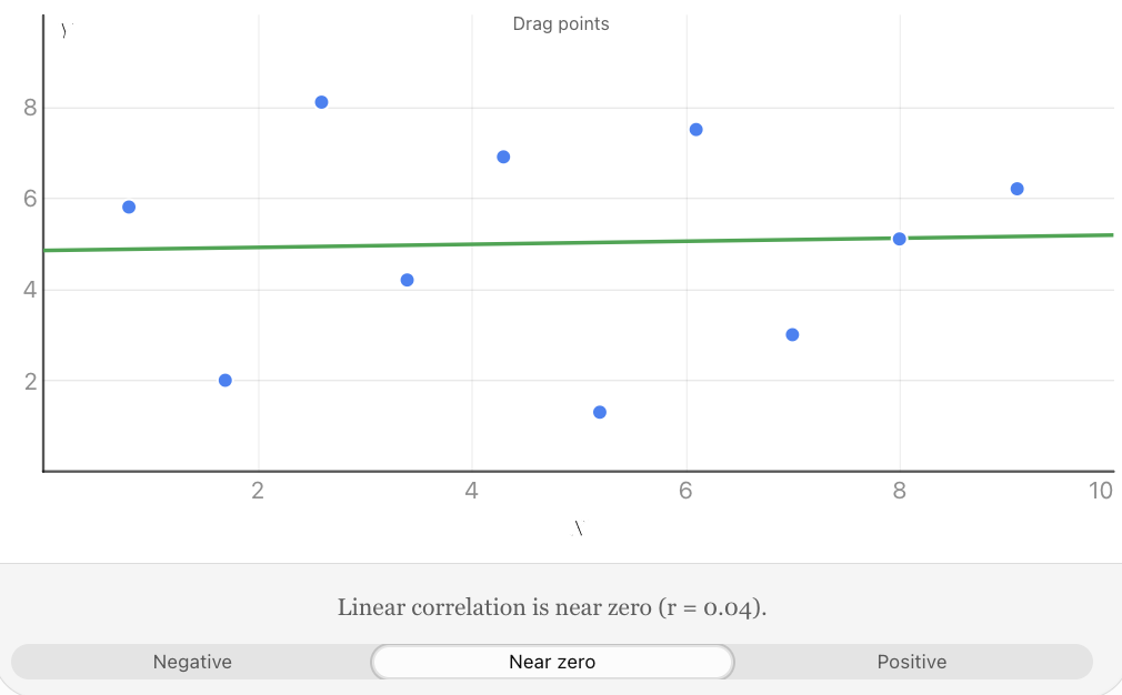
Explore the positive, negative, and uncorrelated patterns. Move individual points and observe how the correlation coefficient changes.
The strength of a relationship is different from its direction. A strong negative correlation can be just as strong as a strong positive correlation.
The Pearson Correlation Coefficient
Visual inspection of a scatter plot is useful, but statisticians often need a numerical measurement.
The Pearson correlation coefficient, represented by r, measures the strength and direction of a linear relationship between two quantitative variables.
Its value is always between −1 and +1.
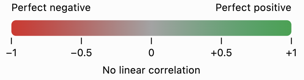
The main interpretations are:
Value of r
Interpretation
+1
Perfect positive linear correlation
+0.8
Strong positive linear correlation
+0.4
Moderate positive linear correlation
0
No linear correlation
−0.4
Moderate negative linear correlation
−0.8
Strong negative linear correlation
−1
Perfect negative linear correlation
These descriptions are approximate. There is no universally accepted boundary between weak, moderate, and strong correlation; interpretations depend on the field and context.
Calculating Pearson's r
The computational formula is:
\[ r=\frac{n\sum xy-(\sum x)(\sum y)} {\sqrt{[n\sum x^2-(\sum x)^2][n\sum y^2-(\sum y)^2]}} \]Where:
-
n = number of paired observations
-
Σx = sum of all x-values
-
Σy = sum of all y-values
-
Σxy = sum of the products of paired values
-
Σx² = sum of the squared x-values
-
Σy² = sum of the squared y-values
The symbol Σ means "sum of."
This formula is suitable when both variables vary and the observations are paired.
Worked Example: Calculating a Correlation Coefficient
Five students complete a practice exercise. Their study time and scores are recorded.
x (hours)
y (score)
x²
y²
xy
1
2
1
4
2
2
3
4
9
6
3
5
9
25
15
4
4
16
16
16
5
6
25
36
30
15
20
55
90
69
Step 1: Identify the totals.
n = 5
Σx = 15
Σy = 20
Σx² = 55
Σy² = 90
Σxy = 69
Step 2: Substitute into the formula.
\[ r=\frac{5(69)-(15)(20)} {\sqrt{[5(55)-15^2][5(90)-20^2]}} \]Step 3: Simplify.
\[ r=\frac{345-300}{\sqrt{(275-225)(450-400)}} \]\[ r=\frac{45}{\sqrt{2500}}=\frac{45}{50} \]\[ \boxed{r=0.90} \]Interpretation: There is a strong positive linear correlation between study time and exercise score in this small dataset.
Students who studied for longer generally achieved higher scores, although the relationship was not perfect.
Calculating Correlation Using Technology
For larger datasets, calculations are usually completed using a spreadsheet, graphing calculator, or statistical software.
In Excel or Google Sheets, if the x-values are in cells A2:A11 and y-values are in B2:B11, enter:
=CORREL(A2:A11,B2:B11)The spreadsheet calculates Pearson's r automatically.
The correlation coefficient measures association; it does not indicate which variable causes the other.
Interpreting Relationships Between Variables
A scatter plot provides more information than simply whether a correlation is positive or negative.
When analysing a scatter plot, consider five important features.
Direction
Does the relationship increase, decrease, or show no consistent linear trend?
Strength
How closely do the points follow the overall pattern?
Form
Is the relationship approximately linear or nonlinear?
A linear relationship follows an approximately straight-line pattern. A nonlinear relationship may follow a curve.
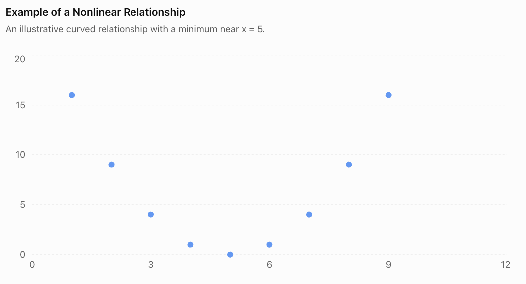
The points form a U-shaped pattern. There is a clear relationship, even though the Pearson correlation coefficient is zero for this symmetric dataset.
This demonstrates why we should inspect the scatter plot before relying on r.
Outliers
An outlier is a point that lies unusually far from the overall pattern.
An outlier may result from measurement error, incorrect data entry, an unusual event, or genuine variation.
Outliers can substantially affect Pearson's correlation coefficient.
Clusters and Subgroups
Sometimes a scatter plot contains separate groups of points.
For example, data from two different age groups might form two clusters. A correlation calculated using all the data may hide important differences within the groups.
When possible, examine the relationship within relevant subgroups as well as across the full dataset.
Lines of Best Fit
A line of best fit, or regression line, summarises an approximately linear relationship between two variables.
It can be used to estimate the value of y for a given x.
A linear model is commonly written as:
\[ y=mx+b \]Where:
-
m = slope of the line
-
b = y-intercept
The slope indicates the predicted change in y for each one-unit increase in x.
Worked Example: Predicting Examination Scores
Suppose a regression model relating study time to examination score is:
\[ y=7x+35 \]Where x represents study time in hours and y represents predicted examination score.
Predict the score for a student who studies for 6 hours.
Substitute x = 6:
\[ y=7(6)+35 \]\[ y=42+35=\boxed{77} \]The predicted score is 77%.
This is a model-based prediction, not a guarantee.
Interpolation and Extrapolation
Interpolation means predicting within the range of observed data.
Extrapolation means predicting beyond the observed range.
For example, if study times were measured from 1 to 8 hours:
-
Predicting the score for 6 hours is interpolation.
-
Predicting the score for 20 hours is extrapolation.
Extrapolation is generally less reliable because the relationship may change outside the observed range. A linear examination-score model, for example, cannot reasonably predict scores above 100%.
Correlation Does Not Imply Causation
One of the most important principles in statistics is that a relationship between two variables does not automatically mean that one variable causes the other.
Correlation means two variables are statistically associated.
Causation means a change in one variable produces a change in another.
Example: Ice Cream Sales and Drowning Incidents
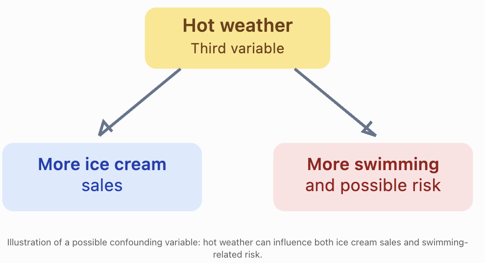
During hotter weather, both ice cream sales and swimming activity may increase. Drowning incidents may also increase when more people are swimming.
A statistical study might find a positive correlation between ice cream sales and drowning incidents.
Does buying ice cream cause drowning?
No.
A third variable, such as hot weather, may help explain the association.
Other Reasons Correlation May Not Establish Causation
Reverse causation: The proposed direction of cause and effect may be incorrect. For example, a relationship between anxiety and poor sleep could involve effects in both directions.
Confounding variables: A third factor may influence both variables.
Coincidence: Two variables may be correlated by chance, particularly when many comparisons are tested.
Selection bias: The way participants or observations are selected may produce a misleading relationship.
How Can Causation Be Investigated?
Researchers can strengthen causal conclusions by using:
-
Randomised controlled experiments, where appropriate and ethical.
-
Longitudinal studies that examine how variables change over time.
-
Careful measurement and control of confounding variables.
-
Replication of findings in different populations.
-
Plausible scientific explanations supported by additional evidence.
Even a very high correlation coefficient, such as r = 0.99, is not by itself proof of causation.
Real-World Applications
Meteorology
Scientists investigate relationships between temperature, humidity, rainfall, and atmospheric pressure. Scatter plots can help identify patterns and evaluate weather models.
Sports Science
Researchers compare exercise intensity with heart rate, oxygen consumption, and recovery time to understand athletic performance.
Economics and Property
Analysts examine associations between property size, location, age, and selling price. Regression models can support price estimates.
Environmental Science
Scientists investigate relationships between pollution levels, water temperature, and aquatic biodiversity. Correlations can help identify environmental questions requiring further investigation.
Common Mistakes
Common mistake
Correction
Assuming positive correlation means a strong relationship
Positive describes direction, not strength.
Thinking r = −0.9 is weaker than r = +0.5
The absolute value of r determines linear strength; 0.9 is stronger than 0.5.
Assuming r = 0 means there is no relationship
There may be a nonlinear relationship.
Connecting every point in a scatter plot
Generally plot the points separately and examine the overall pattern.
Claiming that correlation proves causation
Consider confounding variables, reverse causation, and other explanations.
Ignoring unusual points
Outliers can greatly change the correlation coefficient.
Making predictions far beyond observed values
Extrapolation may produce unrealistic predictions.
Calculating r from unpaired or incorrectly matched observations
Each x-value must be matched with its corresponding y-value.
Key Terms
-
Scatter plot: A graph showing pairs of numerical observations as points.
-
Bivariate data: Data involving two variables measured together.
-
Explanatory variable: A variable used to help explain or predict another variable.
-
Response variable: The variable being investigated or predicted.
-
Correlation: A statistical association between variables.
-
Positive correlation: An association in which larger values of one variable tend to accompany larger values of another.
-
Negative correlation: An association in which larger values of one variable tend to accompany smaller values of another.
-
Linear correlation: An association described by an approximately straight-line pattern.
-
Pearson correlation coefficient (r): A numerical measure of the direction and strength of a linear relationship.
-
Outlier: An observation that lies unusually far from the overall pattern.
-
Line of best fit: A line used to summarise and predict an approximately linear relationship.
-
Regression: A statistical method for modelling relationships between variables.
-
Interpolation: Prediction within the observed data range.
-
Extrapolation: Prediction outside the observed data range.
-
Causation: A relationship in which one factor produces a change in another.
-
Confounding variable: A variable that can distort the apparent relationship between the variables being studied.
Key Takeaways
-
Scatter plots display paired quantitative data and help reveal relationships between two variables.
-
Correlation can be positive, negative, or show little or no linear association.
-
Correlation strength depends on how closely the points follow a linear pattern.
-
Pearson's correlation coefficient, r, ranges from −1 to +1.
-
Values of r close to −1 or +1 indicate strong linear correlation; values near zero indicate weak linear correlation.
-
A scatter plot should be inspected for outliers, clusters, and nonlinear patterns before interpreting r.
-
Regression lines can be used to make predictions, but predictions outside the observed range require caution.
-
Correlation alone cannot establish a cause-and-effect relationship.
Check Your Understanding
Question 1: Identifying Correlation
A dataset shows that as the age of a car increases, its resale value generally decreases.
What type of correlation does this represent?
Question 2: Interpreting Strength
Three datasets have correlation coefficients:
-
Dataset A: r = 0.92
-
Dataset B: r = −0.75
-
Dataset C: r = 0.18
Which dataset has the strongest linear correlation? Which has the weakest?
Question 3: Constructing a Scatter Plot
The table shows the number of hours students spend exercising each week and their resting heart rates.
Exercise (hours)
Resting heart rate (bpm)
1
82
2
79
3
75
4
73
5
69
6
66
Construct a scatter plot, identify the correlation direction, and describe its strength.
Question 4: Calculating Pearson's r
Calculate the Pearson correlation coefficient for the following dataset.
x
y
1
3
2
5
3
4
4
7
Interpret your result.
Question 5: Correlation and Causation
A researcher discovers that cities with more firefighters tend to experience greater total property damage from fires.
A newspaper concludes that employing more firefighters causes greater property damage.
Explain why this conclusion is not justified.
Question 6: Evaluating a Statistical Relationship
A scatter plot of x and y shows a clear U-shaped pattern.
The Pearson correlation coefficient is r = 0.02.
A student concludes that x and y are unrelated.
Explain the problem with this conclusion.
Question 7: Making Predictions
A regression model predicts electricity consumption using:
y = 12x + 150
Where x is the average daily temperature in °C and y is daily electricity consumption in kWh.
Calculate the predicted electricity consumption at 25°C.
Explain why using this model to predict consumption at 70°C might be unreliable if the observed temperatures ranged from 15°C to 35°C.
Fully Worked Answers
Answer 1
The relationship is a negative correlation.
As car age increases, resale value generally decreases.
Answer 2
Compare the absolute values:
Dataset
r
Absolute value
A
0.92
0.92
B
−0.75
0.75
C
0.18
0.18
Dataset A has the strongest linear correlation.
Dataset C has the weakest linear correlation.
The negative sign for Dataset B describes direction, not weakness.
Answer 3
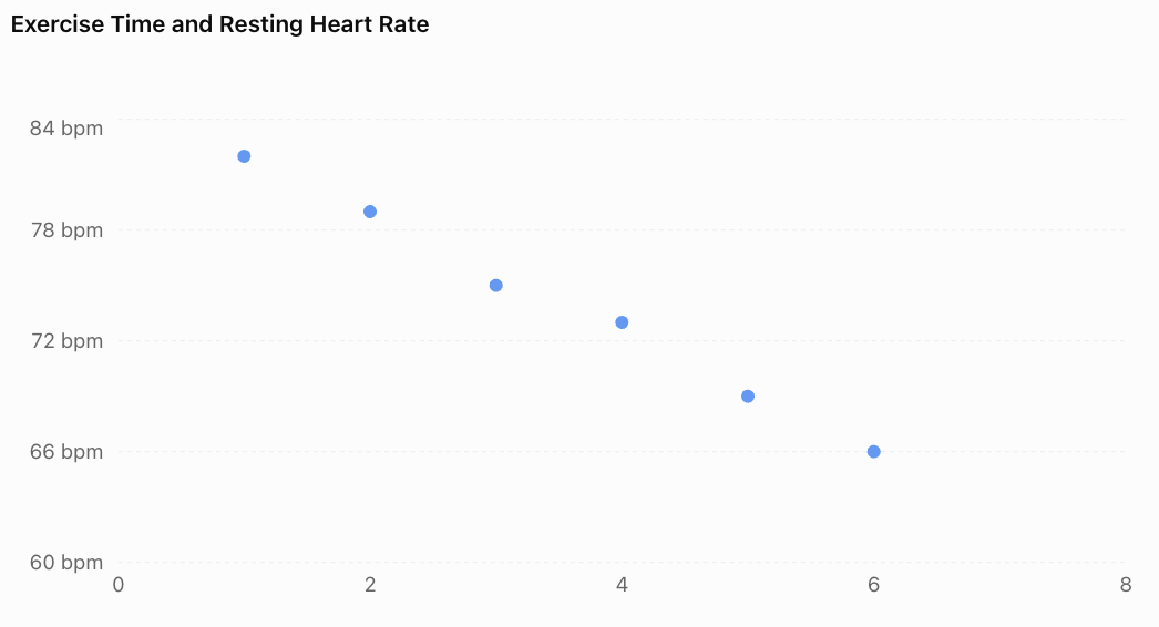
The graph shows a strong negative linear correlation.
As weekly exercise time increases, resting heart rate tends to decrease in this dataset.
This does not establish that exercise time alone caused the differences in resting heart rate.
Answer 4
First calculate the required totals.
x
y
x²
y²
xy
1
3
1
9
3
2
5
4
25
10
3
4
9
16
12
4
7
16
49
28
10
16
30
99
53
n = 4
Substitute:
\[ r=\frac{4(53)-(10)(16)} {\sqrt{[4(30)-10^2][4(99)-16^2]}} \]\[ r=\frac{212-160}{\sqrt{(120-100)(396-256)}} \]\[ r=\frac{52}{\sqrt{2800}} \]\[ \boxed{r\approx0.983} \]The result indicates a very strong positive linear correlation.
Answer 5
Cities with more firefighters may be larger or experience more fires, including more serious fires.
These factors could explain why they also experience greater total property damage.
The correlation does not demonstrate that firefighters cause damage.
A better investigation would consider city size, number of fires, fire severity, building density, and other relevant variables.
Answer 6
Pearson's r measures linear correlation.
A U-shaped relationship is nonlinear. Therefore, r can be close to zero even when the variables have a clear mathematical relationship.
The student should examine the scatter plot and consider a nonlinear model rather than concluding that the variables are unrelated.
Answer 7
Given:
y = 12x + 150
Substitute x = 25:
y = 12(25) + 150
y = 300 + 150
Predicted electricity consumption = 450 kWh.
Predicting at 70°C would be extrapolation because 70°C lies far outside the observed range of 15°C to 35°C.
The original linear relationship may not continue at extreme temperatures, making the prediction unreliable.
Final Reflection
Scatter plots and correlation provide powerful tools for exploring relationships in data. They help us identify patterns, describe the strength and direction of associations, and make informed predictions.
However, responsible statistical reasoning requires more than calculating a correlation coefficient. We must examine the shape of the data, recognise unusual observations, evaluate the reliability of predictions, and consider alternative explanations.
The most important distinction is that a statistical relationship is evidence of association, not automatic proof of cause and effect.
-