Statistical Inference
4. Comparing Populations
Learning outcomes
- I can compare two datasets statistically.
- I can interpret differences between populations.
- I can evaluate statistical evidence.
- I can apply comparative statistical methods.
- I can communicate statistical findings.
Introduction
Imagine that two schools use different teaching methods to help students prepare for a mathematics examination. School A uses traditional classroom instruction, while School B introduces interactive learning activities.
At the end of the term, both schools collect their students' examination scores. School B has a higher average score, but does this necessarily mean that its teaching method is better?
To answer this question, we need to compare the two datasets statistically.
Comparing populations involves examining data from two or more groups to identify similarities, differences, patterns, and relationships. Statistical comparisons help us determine whether observed differences are meaningful or could reasonably be explained by random variation.
These methods are important in education, medicine, business, environmental science, economics, and scientific research.
By comparing populations, we can investigate questions such as:
-
Do students using one learning method achieve higher examination scores?
-
Does a new medicine reduce blood pressure more effectively than an existing treatment?
-
Do two cities experience different average temperatures?
-
Is the average income different between two regions?
-
Does a new manufacturing process produce more consistent products?
A good statistical comparison involves more than simply identifying which group has the higher average. We must also consider variation, sample size, uncertainty, statistical significance, and the practical importance of any differences.
What Does It Mean to Compare Populations?
A population is the complete group of individuals, objects, or observations that we want to study.
A sample is a smaller group selected from that population.
For example:
-
Population A: All students attending School A.
-
Population B: All students attending School B.
-
Sample A: 50 students randomly selected from School A.
-
Sample B: 50 students randomly selected from School B.
We can compare these samples to estimate differences between the two populations.
However, because samples do not necessarily represent their populations perfectly, we must account for sampling uncertainty.
Population Parameters and Sample Statistics
A population parameter describes a characteristic of an entire population.
A sample statistic describes a characteristic calculated from a sample.
|
Characteristic |
Population |
Sample |
|---|---|---|
|
Mean |
μ |
x̄ |
|
Standard deviation |
σ |
s |
|
Proportion |
p |
p̂ |
|
Number of observations |
N |
n |
When comparing two populations, we often investigate the difference between their means:
μ₁ − μ₂
Because population means are usually unknown, we estimate this difference using sample means:
x̄₁ − x̄₂
Example
Suppose two schools have the following average examination scores:
School A: x̄₁ = 72
School B: x̄₂ = 78
Difference = 78 − 72 = 6 marks
School B's sample average is 6 marks higher.
However, this difference alone does not establish that School B's entire population performs better. We need to examine the spread of scores, sample sizes, and uncertainty.
Comparing Measures of Central Tendency
Measures of central tendency describe the typical or central value of a dataset.
The three most common measures are the mean, median, and mode.
Comparing Means
The mean is the arithmetic average.
Mean = Sum of all values ÷ Number of values
x̄ = Σx / n
Consider two groups of students.
Group A scores:
60, 65, 70, 75, 80
Group B scores:
65, 70, 75, 80, 85
Group A mean:
x̄₁ = (60 + 65 + 70 + 75 + 80) / 5
x̄₁ = 70
Group B mean:
x̄₂ = (65 + 70 + 75 + 80 + 85) / 5
x̄₂ = 75
Difference:
75 − 70 = 5
Group B has a mean score 5 marks higher than Group A.
Comparing Medians
The median is the middle value when the data are arranged in order.
For Group A:
60, 65, 70, 75, 80
Median = 70
For Group B:
65, 70, 75, 80, 85
Median = 75
The median confirms that Group B has a higher central score.
The median is particularly useful when datasets contain extreme values or are strongly skewed.
Comparing Modes
The mode is the most frequently occurring value.
For example:
Group A: 60, 65, 65, 70, 80
Mode = 65
Group B: 70, 75, 75, 75, 85
Mode = 75
Group B has a higher modal score.
However, modes are not always useful for comparing continuous numerical data because a dataset may have several modes or no repeated values.
Choosing the Appropriate Measure
|
Data characteristics |
Recommended measure |
|---|---|
|
Approximately symmetric, no extreme outliers |
Mean |
|
Strongly skewed |
Median |
|
Contains extreme outliers |
Median |
|
Categorical data |
Mode or proportions |
|
Approximately normal numerical data |
Mean and standard deviation |
The choice of measure affects how we interpret differences between populations.
Comparing Measures of Spread
Two populations can have identical means but very different distributions.
Consider two classes:
Class A scores:
68, 69, 70, 71, 72
Class B scores:
40, 55, 70, 85, 100
Both classes have a mean of 70.
However, Class A's scores are tightly grouped around the mean, while Class B's scores vary considerably.
Range
The range measures the difference between the maximum and minimum values.
Range = Maximum − Minimum
Class A:
Range = 72 − 68 = 4
Class B:
Range = 100 − 40 = 60
Class B has a much larger range.
Interquartile Range
The interquartile range (IQR) measures the spread of the middle 50% of a dataset.
IQR = Q₃ − Q₁
Here:
-
Q₁ is the first quartile (25th percentile).
-
Q₃ is the third quartile (75th percentile).
The IQR is useful when comparing skewed distributions because it is less sensitive to extreme values than the range.
Standard Deviation
Standard deviation measures how far observations typically lie from the mean.
For a sample:
s = √[Σ(x − x̄)² / (n − 1)]
A small standard deviation indicates that values are closely grouped around the mean.
A large standard deviation indicates greater variability.
Worked Example
Suppose:
Class A: Mean = 70, standard deviation = 5
Class B: Mean = 70, standard deviation = 15
Although both classes have the same mean, Class B has greater variation.
This suggests that student performance in Class A is more consistent.
Illustration: Two populations with equal means but different standard deviations
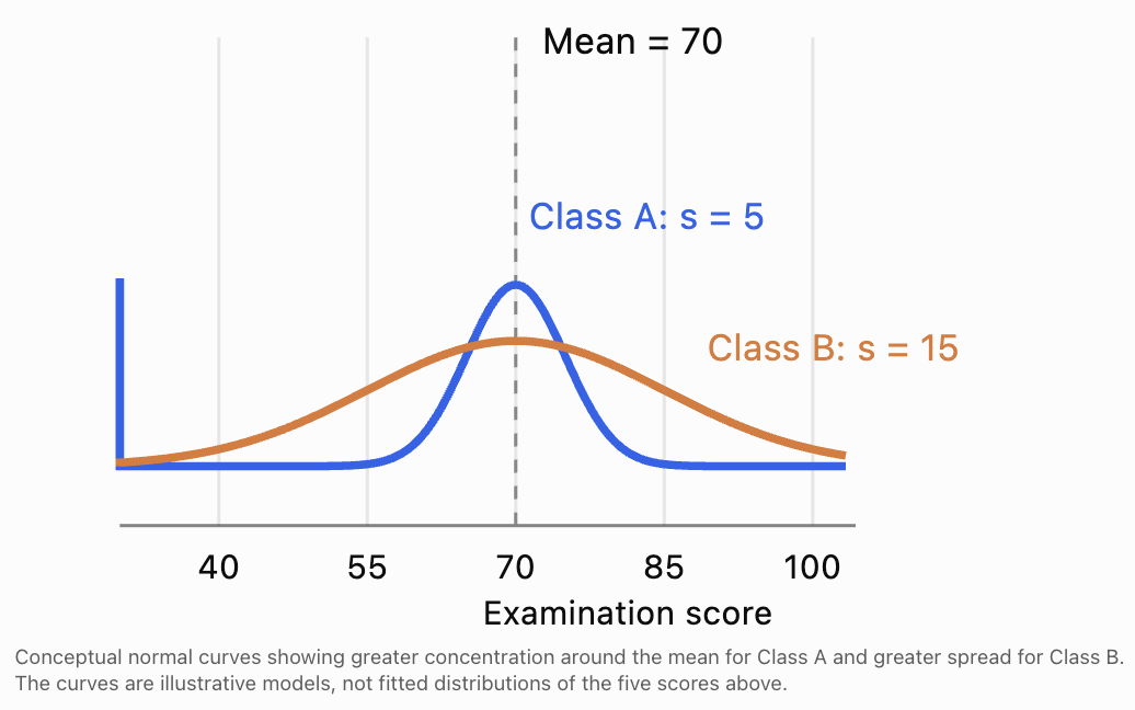
Important: A higher mean does not necessarily indicate a more desirable population. The amount of variation may be equally important.
Interpreting Differences Between Populations
When comparing populations, we should examine several characteristics.
Difference in Location
Does one population tend to have larger values than the other?
We can compare means or medians to investigate this question.
Difference in Spread
Does one population show more variability?
We can compare standard deviations, ranges, or interquartile ranges.
Difference in Shape
Are the distributions symmetric or skewed?
Does one contain more extreme observations?
Are there several clusters or peaks?
Overlap Between Distributions
Two populations may have different means but still overlap substantially.
For example:
Population A: Mean = 65, SD = 10
Population B: Mean = 70, SD = 10
Although Population B has a higher mean, many individuals in Population A may score higher than individuals in Population B.
A difference between population averages does not imply that every individual in one population has a higher value than every individual in the other.
Using Graphs to Compare Populations
Graphs help us identify differences that may be difficult to recognize from numerical summaries alone.
Side-by-Side Box Plots
Box plots show the median, quartiles, and spread of datasets.
Comparing examination scores using box plots
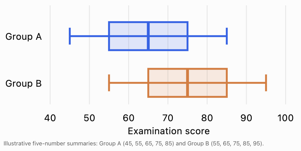
The box plots indicate that Group B generally has higher scores, but both groups have the same IQR:
IQR = 75 − 55 = 20 for Group A
IQR = 85 − 65 = 20 for Group B
The distributions also overlap.
Histograms
Histograms are useful for comparing distribution shapes, including skewness, clustering, and possible outliers.
When comparing histograms, use consistent bin widths and, where possible, the same horizontal scale.
If sample sizes differ, relative frequencies or densities may be more informative than raw frequencies.
Dot Plots
Dot plots are particularly useful for small datasets because they display individual observations.
Choosing a Graph
|
Graph |
Best use |
|---|---|
|
Side-by-side box plots |
Compare medians, quartiles and spread |
|
Histograms |
Compare distribution shapes |
|
Dot plots |
Compare small datasets |
|
Bar charts |
Compare categorical frequencies or proportions |
|
Confidence interval plots |
Compare estimates and their uncertainty |
Comparing Population Means Using Statistical Inference
Descriptive statistics show what happened in our samples.
Inferential statistics help us decide what the sample results suggest about the populations.
One common method is the two-sample t-test.
The Two-Sample t-Test
A two-sample t-test examines whether there is statistical evidence that two population means differ.
Suppose we want to compare the average mathematics scores of students using two teaching methods.
We begin with two hypotheses.
Null hypothesis (H₀):
μ₁ = μ₂
The population means are equal.
Alternative hypothesis (H₁):
μ₁ ≠ μ₂
The population means are different.
The null hypothesis represents the condition against which we test the evidence.
Worked Example: Comparing Teaching Methods
Suppose two independent random samples produce these results:
|
Statistic |
Method A |
Method B |
|---|---|---|
|
Sample size |
40 |
40 |
|
Mean score |
72 |
78 |
|
Standard deviation |
10 |
12 |
We want to determine whether the difference between the population means is statistically significant.
Step 1: Calculate the observed difference
Difference = 78 − 72 = 6
Step 2: Calculate the standard error
For independent samples, Welch's two-sample t-test uses:
SE = √(s₁²/n₁ + s₂²/n₂)
Substitute:
SE = √(10²/40 + 12²/40)
SE = √(2.5 + 3.6)
SE = √6.1
SE ≈ 2.47
Step 3: Calculate the test statistic
t = (x̄₂ − x̄₁) / SE
t = 6 / 2.47
t ≈ 2.43
Step 4: Interpret the result
Using the Welch–Satterthwaite approximation, the degrees of freedom are approximately 75.5.
The two-sided p-value is approximately 0.018.
At the 5% significance level:
p ≈ 0.018 < 0.05
Therefore, we reject the null hypothesis.
There is statistically significant evidence that the population mean examination scores differ.
The sample results suggest Method B is associated with higher scores.
However, this does not establish that Method B caused the improvement. A causal conclusion would require an appropriate experimental design, such as random assignment to teaching methods.
Understanding Statistical Significance
Statistical significance describes whether a result is sufficiently inconsistent with the null hypothesis under a chosen statistical test.
A common significance level is:
α = 0.05
The decision rule is:
-
If p ≤ 0.05, reject H₀.
-
If p > 0.05, do not reject H₀.
A p-value is the probability, assuming the null hypothesis and the statistical model are true, of obtaining a test statistic at least as extreme as the one observed.
It is not the probability that the null hypothesis is true.
Statistical Significance Versus Practical Significance
A statistically significant result is not necessarily important in practical terms.
For example, a large study may find that one teaching method increases the average examination score by only 0.3 marks.
This difference could be statistically significant because the sample size is very large.
However, an improvement of 0.3 marks might have little educational importance.
Conversely, a small study might identify a potentially important difference but lack sufficient statistical power to establish significance.
Therefore, we should consider:
-
The size of the difference.
-
The uncertainty in the estimate.
-
The sample size.
-
The practical consequences.
-
The quality of the study design.
Comparing Populations Using Confidence Intervals
A confidence interval provides a range of plausible values for a population parameter, based on the data and statistical model.
When comparing populations, we can construct a confidence interval for the difference between population means.
For independent samples, an approximate confidence interval is:
(x̄₂ − x̄₁) ± t* × SE
Here:
-
x̄₂ − x̄₁ is the observed difference.
-
t* is the appropriate critical value.
-
SE is the standard error of the difference.
Worked Example
Using our previous teaching-method data:
Observed difference = 6
SE ≈ 2.47
For a 95% confidence interval with approximately 75.5 degrees of freedom:
t* ≈ 1.99
Margin of error:
ME = 1.99 × 2.47
ME ≈ 4.91
Confidence interval:
6 ± 4.91
Lower limit:
6 − 4.91 = 1.09
Upper limit:
6 + 4.91 = 10.91
Therefore, the approximate 95% confidence interval is:
(1.09, 10.91) marks
Interpretation
We are 95% confident that the population mean score for Method B is between approximately 1.09 and 10.91 marks higher than that for Method A, under the assumptions of the analysis.
Because the interval does not contain zero, it supports the conclusion that the population means differ at the 5% significance level in a corresponding two-sided test.
A 95% confidence level means that the method used to construct the interval would capture the true population difference in approximately 95% of repeated samples under the model assumptions.
It does not mean that 95% of individual students have scores within this interval.
Understanding Effect Size
Statistical significance indicates whether there is evidence of a difference.
Effect size describes how large that difference is.
One commonly used measure for numerical data is Cohen's d.
For two independent groups:
d = (x̄₂ − x̄₁) / sₚ
where sₚ is the pooled standard deviation.
For equal sample sizes:
sₚ = √[(s₁² + s₂²)/2]
Worked Example
Using the teaching-method data:
sₚ = √[(10² + 12²)/2]
sₚ = √122
sₚ ≈ 11.05
Cohen's d:
d = 6 / 11.05
d ≈ 0.54
This indicates that the difference between the sample means is approximately 0.54 pooled standard deviations.
A commonly used, approximate interpretation is:
|
Cohen's d |
Conventional description |
|---|---|
|
0.2 |
Small |
|
0.5 |
Medium |
|
0.8 |
Large |
These are guidelines rather than universal rules. The importance of an effect depends on its context.
In this example, the observed effect is approximately medium according to these conventional benchmarks.
Comparing Population Proportions
Not every comparison involves numerical averages.
Sometimes we want to compare proportions.
For example, suppose two schools use different revision programs.
School A:
80 students passed out of 100.
School B:
90 students passed out of 100.
Step 1: Calculate Sample Proportions
School A:
p̂₁ = 80/100 = 0.80
School B:
p̂₂ = 90/100 = 0.90
Step 2: Calculate the Difference
p̂₂ − p̂₁ = 0.90 − 0.80
Difference = 0.10
School B has a pass rate 10 percentage points higher.
Step 3: Calculate the Standard Error
For an estimated difference in proportions:
SE = √[p̂₁(1 − p̂₁)/n₁ + p̂₂(1 − p̂₂)/n₂]
SE = √[(0.80 × 0.20)/100 + (0.90 × 0.10)/100]
SE = √(0.0016 + 0.0009)
SE = 0.05
Step 4: Calculate an Approximate 95% Confidence Interval
Difference ± 1.96 × SE
0.10 ± 1.96 × 0.05
0.10 ± 0.098
Confidence interval:
(0.002, 0.198)
This approximate unpooled Wald interval suggests that School B's population pass rate could be between 0.2 and 19.8 percentage points higher than School A's.
However, the lower endpoint is very close to zero, and the Wald method can be inaccurate in some situations. A score-based confidence interval is often preferable for formal analysis.
When testing equality of proportions, a pooled standard error is commonly used instead.
Paired Versus Independent Comparisons
An important decision is whether the observations in two datasets are independent or paired.
Independent Samples
Independent samples contain observations from separate, unrelated individuals or units.
Examples:
-
Comparing students from two different schools.
-
Comparing patients randomly assigned to different treatments.
-
Comparing products from two independent factories.
Common methods include:
-
Independent-samples t-test.
-
Welch's t-test.
-
Mann–Whitney U test, for appropriate distributional comparisons.
-
Two-proportion z-test.
Paired Samples
Paired samples contain related observations.
Examples:
-
Students' scores before and after a revision course.
-
Blood pressure measurements from the same patients before and after treatment.
-
Measurements from matched pairs of participants.
For paired samples, we first calculate the difference within each pair.
Difference = After − Before
Then we analyse those differences.
Worked Example: Before-and-After Scores
Five students complete a mathematics revision program.
|
Student |
Before |
After |
Difference |
|---|---|---|---|
|
A |
60 |
68 |
+8 |
|
B |
65 |
70 |
+5 |
|
C |
70 |
78 |
+8 |
|
D |
72 |
80 |
+8 |
|
E |
75 |
81 |
+6 |
Mean difference:
d̄ = (8 + 5 + 8 + 8 + 6) / 5
d̄ = 7
The students improved by an average of 7 marks.
A paired t-test could investigate whether there is evidence of a nonzero population mean improvement, provided its assumptions are appropriate.
Using the differences:
5, 6, 8, 8, 8
Sample standard deviation:
s_d = √[Σ(d − 7)² / 4]
s_d = √(8/4)
s_d ≈ 1.41
Standard error:
SE = 1.41 / √5 ≈ 0.632
Test statistic:
t = 7 / 0.632 ≈ 11.07
Degrees of freedom = 4
This provides strong evidence of a positive mean change under the paired t-test assumptions.
However, a small sample of five students limits generalization, and without a control group we cannot conclude that the revision program alone caused the improvement.
Evaluating the Quality of Statistical Evidence
Statistical calculations are only one part of comparing populations.
We must also evaluate whether the evidence is reliable.
Sample Size
Larger samples generally produce more precise estimates, assuming appropriate sampling methods.
Small samples often have greater uncertainty and are more sensitive to unusual observations.
Representative Sampling
A sample should reflect the population being studied.
For example, comparing only the highest-achieving students in one school with randomly selected students in another would produce a biased comparison.
Random sampling can reduce selection bias, although it does not eliminate every source of bias.
Confounding Variables
A confounding variable is a factor related to both the group or exposure being studied and the outcome, potentially distorting their relationship.
For example, differences in examination scores might be associated with:
-
Previous academic achievement.
-
Access to tutoring.
-
Student attendance.
-
Socioeconomic conditions.
-
Study time.
A comparison that ignores important confounding variables may lead to misleading conclusions.
Assumptions of Statistical Tests
Statistical methods depend on assumptions.
For example, a two-sample t-test generally requires:
-
Independent observations within and between groups.
-
Numerical outcomes.
-
Approximately normal sampling distributions of the means, often supported by sufficiently large samples or suitable underlying distributions.
-
No extreme data problems that invalidate the procedure.
Welch's t-test does not require equal population variances.
A paired t-test instead requires independent pairs and a suitable distribution of the within-pair differences.
Outliers
Outliers can substantially affect means and standard deviations.
When outliers are present, consider whether robust methods or comparisons of medians and distributions are more appropriate.
Multiple Comparisons
If researchers perform many statistical tests, the chance of obtaining at least one statistically significant result by chance increases.
Approaches such as Bonferroni correction or false discovery rate control can help address this problem.
Choosing an Appropriate Comparative Statistical Method
Different research questions require different statistical approaches.
|
Research situation |
Possible method |
|---|---|
|
Compare two independent means |
Welch's t-test |
|
Compare means before and after treatment |
Paired t-test |
|
Compare two independent proportions |
Two-proportion z-test |
|
Compare categorical distributions |
Chi-square test |
|
Compare independent ordinal data or distributions |
Mann–Whitney U test |
|
Compare more than two means |
ANOVA |
|
Compare groups while adjusting for other variables |
Regression or ANCOVA |
The correct method depends on the research question, measurement scale, sampling design, assumptions, and type of comparison.
For example, the Mann–Whitney U test is often described as a test of medians, but that interpretation requires additional distributional assumptions. More generally, it compares relative ranks or stochastic ordering.
Communicating Statistical Findings
A good statistical report should explain both the calculations and their meaning.
A Clear Reporting Structure
When comparing populations, include:
-
Research question: What populations or groups are being compared?
-
Descriptive statistics: What are the sample sizes, means, medians, proportions, and measures of spread?
-
Statistical method: Which test or estimation procedure was used, and why?
-
Results: What were the estimated difference, confidence interval, test statistic, and p-value where appropriate?
-
Interpretation: What do the findings suggest in the context of the investigation?
-
Limitations: What factors could affect the reliability or generalizability of the conclusions?
Example Statistical Report
A comparison of examination scores was conducted using two independent samples of 40 students. Students taught using Method A had a mean score of 72 (SD = 10), while those taught using Method B had a mean score of 78 (SD = 12). A Welch two-sample t-test found a statistically significant difference between the group means, t ≈ 2.43, p ≈ 0.018. The estimated mean difference was 6 marks, with an approximate 95% confidence interval of 1.09 to 10.91 marks. These results suggest that Method B is associated with higher examination scores. However, further information about the sampling and allocation procedures is required before drawing causal conclusions.
Notice that this report does not simply state that Method B is better.
It provides numerical evidence, identifies the statistical method, interprets the results, and acknowledges limitations.
Real-World Applications
Medicine: Comparing Treatments
Researchers may compare blood pressure reductions in patients receiving two different treatments.
They can examine mean reductions, variability, confidence intervals, and possible adverse effects.
A statistically significant difference may not necessarily be clinically meaningful.
Education: Evaluating Teaching Strategies
Schools may compare examination results, attendance rates, or student progress under different teaching approaches.
Researchers must consider previous achievement, class composition, and other potential confounders.
Manufacturing: Comparing Product Quality
Two factories may produce components with the same average dimensions but different standard deviations.
The factory with lower variation may produce more consistently sized components.
Environmental Science: Comparing Pollution Levels
Scientists may compare average particulate pollution concentrations between two cities.
However, seasonal differences, weather, measurement methods, and monitoring locations can affect the comparison.
Business: Comparing Conversion Rates
An online business might compare the proportion of visitors who register for an account under two different website designs.
For example:
Design A: 120 registrations from 2,000 visitors = 6%
Design B: 165 registrations from 2,000 visitors = 8.25%
Observed difference:
8.25% − 6% = 2.25 percentage points
Relative increase:
(8.25 − 6) / 6 × 100% = 37.5%
This is a 37.5% relative increase in the observed registration rate, not an increase of 37.5 percentage points.
A properly randomized A/B test can help determine whether the design change caused an improvement.
Common Mistakes
Mistake 1: Comparing means without considering variation
Two groups can have different means but substantial overlap.
Always examine standard deviations, distributions, and uncertainty.
Mistake 2: Assuming statistical significance means practical importance
A very small difference may be statistically significant with a sufficiently large sample.
Consider effect size and context.
Mistake 3: Interpreting a nonsignificant result as proof of equality
Failing to reject the null hypothesis does not establish that two populations are identical.
The data may be insufficiently precise to detect an important difference.
Mistake 4: Using an independent-samples test for paired data
Before-and-after measurements from the same individuals are related.
A paired analysis is generally more appropriate.
Mistake 5: Ignoring sample bias
A large biased sample may produce a precise estimate of the wrong quantity.
Sampling quality is essential.
Mistake 6: Confusing percentage points and percentage changes
An increase from 20% to 30% is:
-
10 percentage points.
-
A 50% relative increase.
These are different descriptions.
Mistake 7: Claiming causation from observational comparisons
A statistically significant association does not necessarily mean that one variable caused another.
Confounding variables and study design must be considered.
Mistake 8: Misinterpreting confidence intervals
A 95% confidence interval does not mean there is a 95% probability that the fixed population parameter lies in the calculated interval.
The 95% refers to the long-run coverage of the interval-building procedure.
Key Terms
-
Population: The complete group of individuals or observations of interest.
-
Sample: A subset of a population used for statistical analysis.
-
Population parameter: A numerical characteristic of a population.
-
Sample statistic: A numerical characteristic calculated from a sample.
-
Mean: The arithmetic average of a dataset.
-
Median: The middle value of an ordered dataset.
-
Mode: The most frequently occurring value.
-
Range: The difference between the maximum and minimum values.
-
Interquartile range (IQR): The difference between the third and first quartiles.
-
Standard deviation: A measure of variability around the mean.
-
Sampling variability: Variation in sample statistics across different random samples.
-
Standard error: The estimated standard deviation of a statistic's sampling distribution.
-
Null hypothesis: A statistical claim used as the reference point for a hypothesis test.
-
Alternative hypothesis: A competing statistical claim.
-
p-value: The probability, under the null hypothesis and model, of obtaining a test statistic at least as extreme as the observed value.
-
Significance level: A chosen threshold for deciding whether to reject the null hypothesis.
-
Confidence interval: An interval estimate constructed using a method with a specified long-run coverage rate.
-
Effect size: A measure of the magnitude of a statistical relationship or difference.
-
Independent samples: Samples consisting of unrelated observations.
-
Paired samples: Samples containing matched or repeated observations.
-
Confounding variable: A variable that can distort the relationship between an exposure and an outcome.
-
Statistical significance: Evidence against a null hypothesis according to a specified statistical test and significance level.
-
Practical significance: The real-world importance of an observed effect.
Key Takeaways
-
Comparing populations involves examining differences in central tendency, spread, shape, and other statistical characteristics.
-
Sample statistics provide estimates of unknown population parameters.
-
Means and medians describe typical values, while standard deviations and IQRs describe variation.
-
Graphs such as box plots, histograms, and dot plots help reveal patterns and differences.
-
Statistical tests assess how strongly the data contradict a specified null hypothesis.
-
Confidence intervals provide information about both the estimated difference and its uncertainty.
-
Effect sizes help describe the magnitude of differences.
-
Independent and paired data require different analytical approaches.
-
Sample size, bias, confounding variables, and statistical assumptions affect the reliability of conclusions.
-
Clear statistical communication includes numerical evidence, contextual interpretation, and appropriate limitations.
Check Your Understanding
Question 1: Comparing Means
Two groups of students receive the following examination scores.
Group A: 60, 70, 75, 80, 85
Group B: 65, 75, 80, 85, 95
Calculate the mean for each group and determine which group has the higher mean.
Answer
Group A:
Mean = (60 + 70 + 75 + 80 + 85) / 5
Mean = 370 / 5 = 74
Group B:
Mean = (65 + 75 + 80 + 85 + 95) / 5
Mean = 400 / 5 = 80
Difference:
80 − 74 = 6
Group B has a mean score 6 marks higher than Group A.
This describes the observed samples but does not by itself establish a population difference.
Question 2: Comparing Variation
Two datasets have the following characteristics:
Dataset A: Mean = 50, SD = 4
Dataset B: Mean = 50, SD = 12
Which dataset has greater variation?
Answer
Dataset B has greater variation because its standard deviation is larger.
The values in Dataset B tend to be more widely dispersed around the mean.
Both datasets have the same mean, but their consistency differs.
Question 3: Interpreting Statistical Significance
A statistical test comparing two population means produces:
p = 0.032
The significance level is:
α = 0.05
What conclusion should be reached?
Answer
Since:
0.032 < 0.05
We reject the null hypothesis.
There is statistically significant evidence of a difference between the population means, assuming the test and its assumptions are appropriate.
This does not necessarily mean that the difference is large or practically important.
Question 4: Confidence Intervals
A study estimates that the mean difference between two populations is 8 units.
The standard error is 3 units.
Calculate an approximate 95% confidence interval using a critical value of 1.96.
Answer
Confidence interval:
Difference ± 1.96 × SE
= 8 ± 1.96 × 3
= 8 ± 5.88
Lower limit:
8 − 5.88 = 2.12
Upper limit:
8 + 5.88 = 13.88
95% confidence interval: (2.12, 13.88)
Because the interval does not include zero, it suggests a positive population mean difference under the normal approximation.
Question 5: Comparing Proportions
School A has 120 students who pass an examination out of 150 students.
School B has 135 students who pass out of 150.
Calculate the pass rates and their difference.
Answer
School A:
120 / 150 × 100% = 80%
School B:
135 / 150 × 100% = 90%
Difference:
90% − 80% = 10 percentage points
School B's observed pass rate is 10 percentage points higher.
Relative increase:
(90 − 80) / 80 × 100% = 12.5%
Therefore, School B's pass rate is 12.5% higher relative to School A's rate.
Question 6: Choosing a Statistical Method
A researcher measures the reaction times of 30 participants before and after drinking coffee.
Should the researcher use an independent-samples t-test or a paired t-test?
Answer
A paired t-test is appropriate because the same participants are measured twice.
The researcher should calculate each participant's change in reaction time and analyse the differences.
This accounts for the relationship between the two measurements.
Question 7: Evaluating Statistical Evidence
A study reports that a new teaching method improves examination scores by an average of 2 marks.
The difference is statistically significant, with p = 0.001.
Does this prove that the teaching method is educationally important?
Answer
No.
The p-value provides evidence against the null hypothesis but does not describe the educational importance of the difference.
A 2-mark improvement may or may not be meaningful, depending on the examination scale, consequences, costs, and other factors.
We should also examine the confidence interval, effect size, study design, and possible confounding variables.
Question 8: Comparing Two Populations
Two independent samples have the following characteristics:
Population A sample:
n₁ = 50, x̄₁ = 100, s₁ = 15
Population B sample:
n₂ = 50, x̄₂ = 108, s₂ = 20
Calculate the standard error of the difference and the Welch t-statistic.
Answer
Step 1: Calculate the standard error.
SE = √(s₁²/n₁ + s₂²/n₂)
SE = √(15²/50 + 20²/50)
SE = √(225/50 + 400/50)
SE = √(4.5 + 8)
SE = √12.5
SE ≈ 3.54
Step 2: Calculate the difference.
Difference = 108 − 100 = 8
Step 3: Calculate the t-statistic.
t = 8 / 3.54
t ≈ 2.26
This statistic can be used with the appropriate Welch degrees of freedom to calculate a p-value.
The result suggests that Population B may have a higher mean, but a complete inferential conclusion requires the test assumptions, degrees of freedom, and chosen significance level.
Question 9: Identifying Bias
A researcher compares the examination scores of students attending two schools.
For School A, the researcher selects only students enrolled in advanced mathematics classes.
For School B, the researcher selects students randomly from all mathematics classes.
Explain why the comparison may be misleading.
Answer
The samples were selected using different procedures.
School A's sample includes only advanced mathematics students, who may have higher achievement than the overall student population.
School B's sample represents a wider range of students.
Therefore, the observed difference may reflect selection bias rather than a genuine difference between the schools.
A better approach would be to use comparable sampling methods and account for relevant student characteristics.
Question 10: Communicating a Statistical Conclusion
A researcher compares the average daily exercise time of two groups.
Group A:
Mean = 35 minutes
Group B:
Mean = 42 minutes
The estimated difference is 7 minutes, with a 95% confidence interval from 2 to 12 minutes.
Write an appropriate statistical conclusion.
Answer
Group B exercised for an average of 7 minutes longer per day than Group A in the samples studied.
The 95% confidence interval suggests that the population mean difference is plausibly between 2 and 12 minutes, under the statistical model.
Because the confidence interval does not include zero, the results provide evidence of a difference between the population means.
However, the practical importance of this difference depends on the research context, and the reliability of the conclusion depends on the study design, sampling methods, and statistical assumptions.
Final Reflection
Comparing populations is one of the most important applications of statistics because it allows us to move beyond individual observations and investigate broader patterns.
A strong statistical comparison does not simply ask, "Which group has the higher average?"
It also asks:
-
How large is the difference?
-
How much variation exists within each group?
-
How reliable is the evidence?
-
Could the difference be explained by sampling variability or bias?
-
Is the difference meaningful in the real world?
-
What conclusions can we reasonably communicate?
By combining descriptive statistics, graphical analysis, statistical inference, and careful interpretation, we can make informed comparisons and communicate findings accurately and responsibly.