Statistical Inference
| サイト: | Young Education |
| コース: | Statistics |
| ブック: | Statistical Inference |
| 印刷者: | Guest user |
| 日付: | 2026年 11月 9日(月曜日) 16:40 |
1. Confidence Intervals
Learning outcomes
- I can explain the purpose of confidence intervals.
- I can calculate confidence intervals.
- I can interpret confidence levels.
- I can estimate population parameters.
- I can communicate interval estimates.
Introduction
Imagine that a school wants to estimate the average amount of time students spend studying each evening.
Surveying every student may be difficult, expensive, or time-consuming. Instead, the school selects a random sample of 100 students and calculates their average study time.
Suppose the sample mean is 85 minutes.
Does this mean that the true average study time of every student in the school is exactly 85 minutes?
Not necessarily.
Different random samples would usually produce slightly different averages. This natural variation is called sampling variability.
Statistics provides a way to express the uncertainty associated with an estimate. One of the most important tools for doing this is a confidence interval.
A confidence interval provides a range of plausible values for an unknown population parameter, calculated using sample data and a statistical method with a specified confidence level.
For example, a 95% confidence interval for the population mean might be:
79.1 minutes to 90.9 minutes.
This interval provides more information than the sample mean alone because it communicates both the estimate and its uncertainty.
Confidence intervals are widely used in scientific research, education, medicine, economics, engineering, opinion polling, and quality control.
Population Parameters and Sample Statistics
Before calculating confidence intervals, we need to distinguish between a population and a sample.
Population
A population is the complete group of individuals or objects we want to study.
Examples include:
-
All students at a school.
-
All manufactured batteries from a production process.
-
All households in a city.
-
All trees in a forest.
-
All customers of a business.
Sample
A sample is a smaller group selected from the population.
A sample is used to collect information about the population.
Parameter
A population parameter is a numerical characteristic of the entire population.
Common parameters include:
-
μ (mu): population mean.
-
p: population proportion.
-
σ (sigma): population standard deviation.
These parameters are often unknown.
Statistic
A sample statistic is a numerical characteristic calculated from sample data.
Common statistics include:
-
x̄: sample mean.
-
p̂: sample proportion.
-
s: sample standard deviation.
Sample statistics are used to estimate population parameters.
|
Population parameter |
Sample statistic |
|---|---|
|
Mean μ |
Mean x̄ |
|
Proportion p |
Proportion p̂ |
|
Standard deviation σ |
Standard deviation s |
A sample statistic is a point estimate of the corresponding population parameter.
Point Estimates and Interval Estimates
A point estimate provides one numerical value.
An interval estimate provides a range of values.
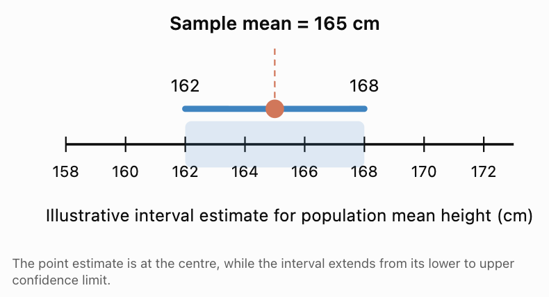
Suppose a random sample of students has an average height of 165 cm.
Point estimate:
μ ≈ 165 cm.
A possible confidence interval might be:
162 cm to 168 cm.
The interval communicates uncertainty about the population mean.
Why Do We Need Confidence Intervals?
Confidence intervals help us:
-
Estimate unknown population parameters.
-
Quantify uncertainty caused by random sampling.
-
Compare the precision of different estimates.
-
Communicate statistical findings.
-
Make decisions using a range rather than a single value.
A point estimate alone may suggest more certainty than the data justify.
A confidence interval provides a more informative summary.
The Structure of a Confidence Interval
Many common confidence intervals follow the form:
Confidence interval = Point estimate ± Margin of error
The margin of error describes how far the interval extends on either side of the point estimate.
More generally:
Margin of error = Critical value × Standard error
Therefore:
Confidence interval = Estimate ± (Critical value × Standard error)
Point Estimate
The sample statistic used to estimate the population parameter.
Critical Value
A multiplier determined by the confidence level and the statistical distribution being used.
Standard Error
A measure of how much a sample statistic varies from sample to sample.
Margin of Error
The amount added to and subtracted from the point estimate to construct the interval.
Worked Example 1: Understanding Margin of Error
A survey estimates that 62% of students prefer digital textbooks.
The reported margin of error is 5 percentage points.
Calculate the interval.
Lower limit:
62% − 5% = 57%.
Upper limit:
62% + 5% = 67%.
Answer: 57% to 67%.
The point estimate is 62%, and the margin of error is 5 percentage points.
This calculation does not by itself establish a confidence level; that depends on how the margin of error was obtained.
Confidence Levels
The confidence level describes the long-run success rate of the method used to construct confidence intervals.
Common confidence levels are:
|
Confidence level |
Approximate z critical value for a two-sided interval |
|---|---|
|
80% |
1.282 |
|
90% |
1.645 |
|
95% |
1.960 |
|
98% |
2.326 |
|
99% |
2.576 |
These z-values apply when a normal critical value is appropriate.
A higher confidence level requires a larger critical value and therefore usually produces a wider interval when the data and method remain unchanged.
What Does 95% Confidence Mean?
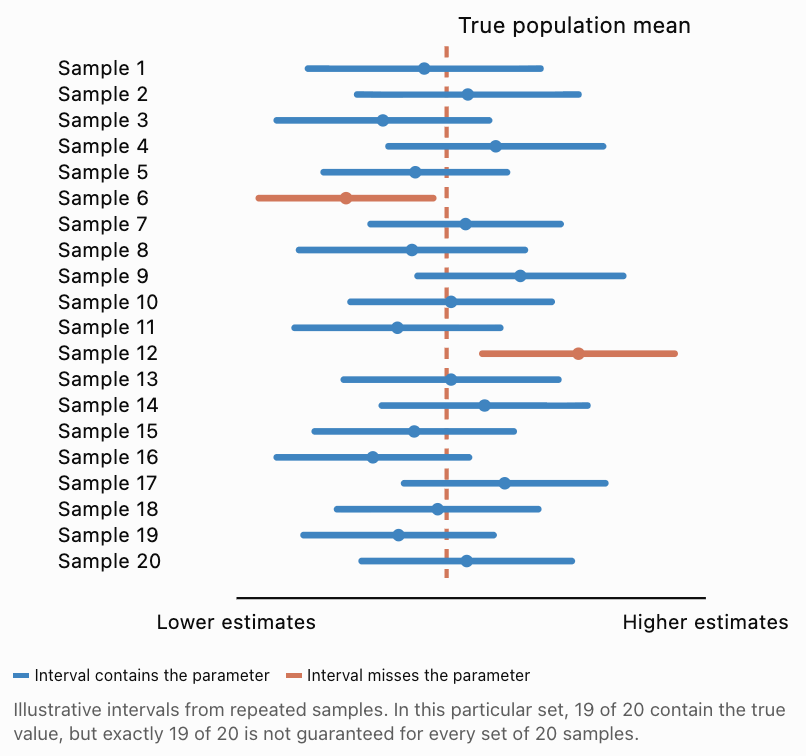
Suppose we repeatedly:
-
Select a random sample from the same population.
-
Calculate a 95% confidence interval using the same valid method.
-
Record whether the interval contains the true population parameter.
Over many repetitions, approximately 95% of the calculated intervals would contain the true parameter.
This is the correct frequentist interpretation of a 95% confidence level.
It does not mean that there is a 95% probability that the fixed population parameter lies inside one particular interval after it has been calculated.
The parameter is treated as fixed; the interval changes from sample to sample.
Repeated 95% confidence intervals (illustrative simulation)
Confidence Level and Interval Width
Explore how the same sample estimate produces different interval widths when the confidence level changes.
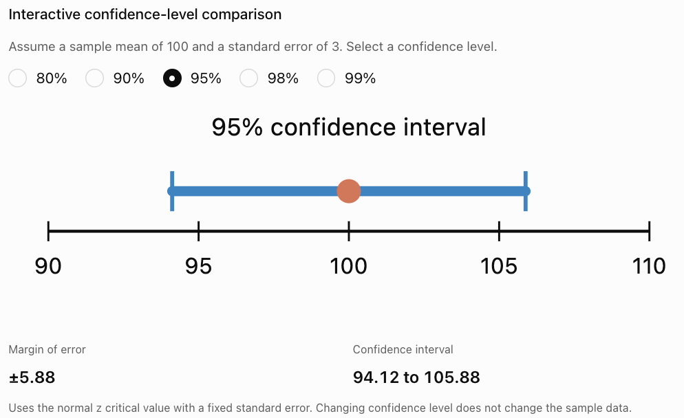
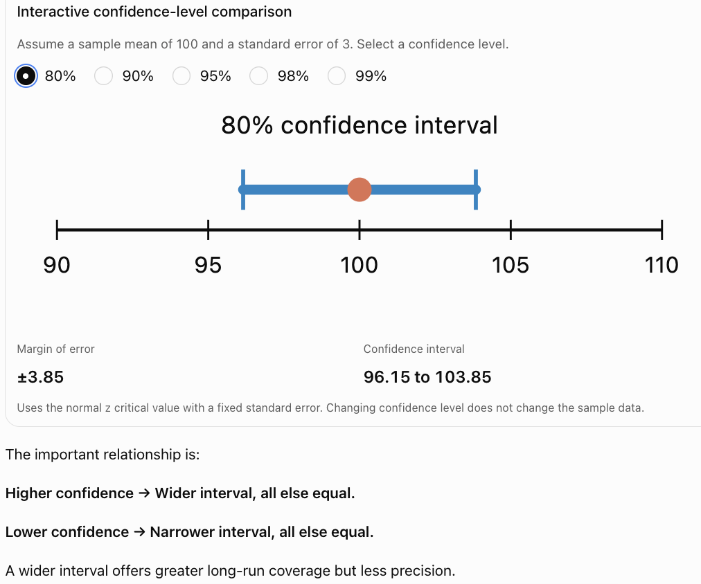
The important relationship is:
Higher confidence → Wider interval, all else equal.
Lower confidence → Narrower interval, all else equal.
A wider interval offers greater long-run coverage but less precision.
Calculating Confidence Intervals for a Population Mean
When estimating a population mean, the appropriate method depends on whether the population standard deviation is known.
Case 1: Population Standard Deviation Is Known
When the population standard deviation σ is known and the sampling distribution of the mean is normal or approximately normal, use the z confidence interval.
Formula:
CI = x̄ ± z* × σ/√n
Where:
-
x̄ = sample mean.
-
z* = critical value.
-
σ = population standard deviation.
-
n = sample size.
-
σ/√n = standard error of the sample mean.
The method assumes independent observations from an appropriate sampling process. A normal population or sufficiently large sample can justify the normal approximation.
Worked Example 2: A 95% Confidence Interval for a Mean
A manufacturer produces batteries.
A random sample of 64 batteries has an average lifetime of 520 hours.
The population standard deviation is known to be 40 hours.
Construct a 95% confidence interval for the population mean battery lifetime.
Step 1: Identify the information
x̄ = 520 hours.
σ = 40 hours.
n = 64.
z* = 1.96.
Step 2: Calculate the standard error
SE = σ/√n
= 40/√64
= 40/8
= 5 hours.
Step 3: Calculate the margin of error
ME = z* × SE
= 1.96 × 5
= 9.8 hours.
Step 4: Calculate the confidence interval
CI = 520 ± 9.8.
Lower limit:
520 − 9.8 = 510.2.
Upper limit:
520 + 9.8 = 529.8.
Answer: 95% CI = (510.2, 529.8) hours.
Interpretation: We are 95% confident that the population mean battery lifetime lies between 510.2 and 529.8 hours, in the sense that the method used has 95% long-run coverage under its assumptions.
Worked Example 3: Comparing 90% and 99% Confidence Intervals
Using the same battery data:
x̄ = 520, SE = 5.
For a 90% interval:
z* = 1.645.
ME = 1.645 × 5 = 8.225.
CI = (511.775, 528.225).
For a 99% interval:
z* = 2.576.
ME = 2.576 × 5 = 12.88.
CI = (507.12, 532.88).
|
Confidence level |
Margin of error |
Confidence interval |
|---|---|---|
|
90% |
8.23 hours |
511.78–528.23 hours |
|
95% |
9.80 hours |
510.20–529.80 hours |
|
99% |
12.88 hours |
507.12–532.88 hours |
Conclusion: The 99% confidence interval is wider because it is designed to achieve a higher long-run coverage rate.
Case 2: Population Standard Deviation Is Unknown
In most real-world investigations, the population standard deviation σ is unknown.
Instead, we use the sample standard deviation s.
For a confidence interval for a population mean, the standard method is the Student's t-distribution.
Formula:
CI = x̄ ± t* × s/√n
Where:
-
x̄ = sample mean.
-
t* = t critical value.
-
s = sample standard deviation.
-
n = sample size.
-
Degrees of freedom = n − 1.
The t-distribution accounts for the additional uncertainty from estimating σ with s.
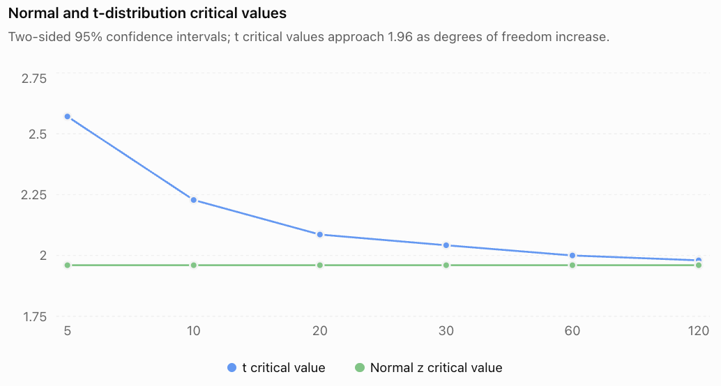
For small samples, the t-distribution has heavier tails than the standard normal distribution, producing larger critical values.
As the degrees of freedom increase, the t-distribution approaches the normal distribution.
When Is a t-Interval Appropriate?
A one-sample t-interval is appropriate when:
-
The sample is randomly selected or otherwise obtained through a defensible sampling design.
-
Observations are independent or sufficiently close to independent.
-
The population is approximately normal for small samples, with no serious outliers.
-
For larger samples, the sampling distribution of the mean is approximately normal.
For sampling without replacement from a finite population, the sample should generally be a small fraction of the population for the usual independent-observations approximation; a common guideline is no more than 10%.
The t-method does not automatically correct for biased sampling or severe outliers.
Worked Example 4: A 95% t-Confidence Interval
A random sample of 16 students records the following summary statistics for time spent completing a homework task:
Sample mean = 42 minutes.
Sample standard deviation = 8 minutes.
Assume the underlying distribution is approximately normal.
Estimate the population mean completion time using a 95% confidence interval.
Step 1: Identify the information
x̄ = 42.
s = 8.
n = 16.
Degrees of freedom:
df = 16 − 1 = 15.
For 95% confidence and 15 degrees of freedom:
t* ≈ 2.131.
Step 2: Calculate standard error
SE = s/√n
= 8/√16
= 2 minutes.
Step 3: Calculate margin of error
ME = 2.131 × 2
= 4.262 minutes.
Step 4: Construct the interval
CI = 42 ± 4.262.
Lower limit = 37.738.
Upper limit = 46.262.
Answer: 95% CI ≈ (37.74, 46.26) minutes.
Interpretation: We are 95% confident that the population mean homework completion time lies between approximately 37.74 and 46.26 minutes.
The confidence statement concerns the population mean, not the completion time of every individual student.
Worked Example 5: Why We Should Not Automatically Use z = 1.96
Consider the same sample:
x̄ = 42, s = 8, n = 16.
If we incorrectly use z = 1.96:
ME = 1.96 × 8/4
= 3.92.
The resulting interval would be:
(38.08, 45.92).
The correct t-based interval is:
(37.74, 46.26).
The z-based interval is narrower because it fails to account appropriately for the uncertainty in estimating the population standard deviation from this small sample.
Conclusion: When σ is unknown, the t-method is generally the appropriate choice for inference about a population mean.
Confidence Intervals for a Population Proportion
Confidence intervals can also estimate population proportions.
For example:
-
The proportion of students who walk to school.
-
The proportion of voters who support a proposal.
-
The proportion of products that are defective.
-
The proportion of households with internet access.
The sample proportion is:
p̂ = x/n
Where:
-
x = number of successes.
-
n = sample size.
A common introductory method is the normal-approximation, or Wald, interval:
CI = p̂ ± z × √(p̂(1 − p̂)/n)*
This method is easiest to calculate by hand but can perform poorly, particularly for small samples or proportions near 0 or 1. In practice, the Wilson score interval is often preferred.
For introductory Wald calculations, check that:
n p̂ ≥ 10
and
n(1 − p̂) ≥ 10.
These conditions help support the normal approximation, although they do not guarantee ideal coverage.
Worked Example 6: A Confidence Interval for a Proportion
A random sample of 400 students finds that 240 prefer online learning resources.
Construct an approximate 95% confidence interval for the population proportion.
Step 1: Calculate the sample proportion
p̂ = 240/400
= 0.60.
Step 2: Check the approximation
n p̂ = 400 × 0.60 = 240.
n(1 − p̂) = 400 × 0.40 = 160.
Both exceed 10.
Step 3: Calculate standard error
SE = √(0.60 × 0.40/400)
= √0.0006
≈ 0.024495.
Step 4: Calculate margin of error
ME = 1.96 × 0.024495
≈ 0.04801.
Step 5: Calculate interval
CI = 0.60 ± 0.04801.
Lower limit ≈ 0.55199.
Upper limit ≈ 0.64801.
Answer: Approximately (0.552, 0.648), or 55.2% to 64.8%.
Interpretation: We are 95% confident that approximately 55.2% to 64.8% of the population of students prefer online learning resources, assuming the sampling method is appropriate.
Worked Example 7: Estimating a Defect Rate
A manufacturer inspects a random sample of 500 products.
Of these, 25 are defective.
Calculate an approximate 95% confidence interval for the population defect proportion.
Step 1: Sample proportion
p̂ = 25/500 = 0.05.
Step 2: Check approximation
n p̂ = 25.
n(1 − p̂) = 475.
Both are at least 10.
Step 3: Standard error
SE = √(0.05 × 0.95/500)
≈ 0.009747.
Step 4: Margin of error
ME = 1.96 × 0.009747
≈ 0.01910.
Step 5: Interval
CI = 0.05 ± 0.01910.
Answer: Approximately (0.0309, 0.0691), or 3.09% to 6.91%.
The sample defect rate is 5%, but the interval shows that the population defect rate could plausibly differ from that estimate.
Selecting the Appropriate Confidence Interval
|
Situation |
Typical method |
Formula |
|---|---|---|
|
Population mean, σ known |
z interval |
x̄ ± z*σ/√n |
|
Population mean, σ unknown |
t interval |
x̄ ± t*s/√n |
|
Population proportion, introductory approximation |
z/Wald interval |
p̂ ± z*√(p̂(1 − p̂)/n) |
Other methods are needed for differences between groups, paired data, very small proportions, and more complicated sampling designs.
The correct formula depends on the parameter, available information, sampling method, and statistical assumptions.
Estimating Population Parameters
Confidence intervals help us estimate unknown population characteristics without measuring every member of the population.
However, a confidence interval is only as trustworthy as the data and assumptions used to construct it.
Sampling Methods Matter
A random sample is generally preferable to a convenience sample because it reduces the risk of systematic selection bias.
For example, a school wants to estimate the average time students spend using their phones.
Surveying only students who attend a technology club may produce an unrepresentative estimate.
Even a very narrow confidence interval based on biased data may be misleading.
Confidence intervals quantify certain forms of sampling uncertainty; they do not automatically account for bias.
How Sample Size Affects Confidence Intervals
For a mean with known population standard deviation:
ME = z*σ/√n.
The sample size n appears under a square root.
Therefore, increasing the sample size reduces the margin of error, provided other factors remain unchanged.
Worked Example 8: Increasing Sample Size
Suppose:
σ = 20.
Confidence level = 95%.
z* = 1.96.
Compare samples of sizes 25, 100, and 400.
For n = 25:
ME = 1.96 × 20/√25
= 7.84.
For n = 100:
ME = 1.96 × 20/√100
= 3.92.
For n = 400:
ME = 1.96 × 20/√400
= 1.96.
|
Sample size |
Margin of error |
|---|---|
|
25 |
±7.84 |
|
100 |
±3.92 |
|
400 |
±1.96 |
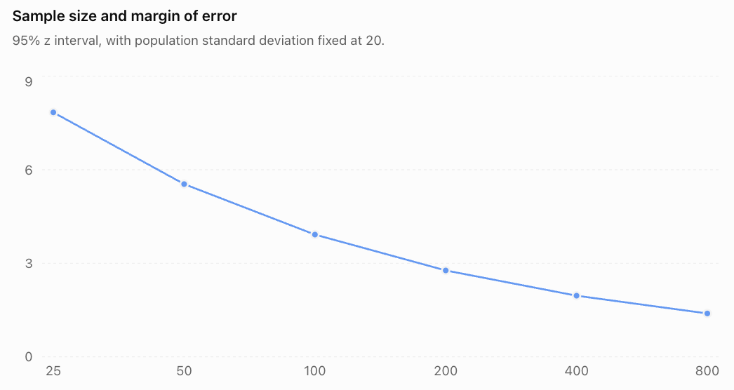
Important result: To halve the margin of error, we generally need four times the sample size.
This is because:
ME ∝ 1/√n.
Calculating a Required Sample Size
Sometimes researchers want to achieve a specified margin of error before collecting data.
For a population mean with known σ:
ME = z*σ/√n.
Rearranging:
√n = z*σ/ME.
Therefore:
**n = (z*σ/ME)²**
Always round the required sample size up to the next whole number.
Worked Example 9: Planning a Survey of a Mean
A researcher wants to estimate the mean mass of a manufactured component.
The population standard deviation is known to be 12 g.
The researcher wants a 95% confidence interval with margin of error no greater than 3 g.
Find the required sample size.
Step 1: Identify the values
z* = 1.96.
σ = 12.
ME = 3.
Step 2: Substitute
n = (1.96 × 12/3)²
= 7.84²
= 61.4656.
Step 3: Round up
Answer: At least 62 components.
Rounding down would not guarantee the target margin of error.
Sample Size for a Population Proportion
For the introductory normal-approximation method, a planning formula is:
**n = z*²p₀(1 − p₀)/ME²**
Where p₀ is an anticipated population proportion.
If no reasonable estimate of the proportion is available, use:
p₀ = 0.5.
This produces the largest value of p₀(1 − p₀) and therefore a conservative sample size under this formula.
Worked Example 10: Planning an Opinion Survey
A researcher wants to estimate a population proportion with:
-
95% confidence.
-
Margin of error no greater than 4 percentage points.
-
No prior estimate of the proportion.
Use p₀ = 0.5.
n = 1.96² × 0.5 × 0.5 / 0.04²
= 3.8416 × 0.25 / 0.0016
= 600.25.
Round up:
Answer: At least 601 respondents.
This assumes a simple random sampling framework and does not include adjustments for nonresponse, clustering, or other design effects.
Interpreting Confidence Intervals Correctly
Calculating a confidence interval is only one part of the statistical process.
A complete interpretation must identify:
-
The population being studied.
-
The parameter being estimated.
-
The confidence level.
-
The lower and upper limits.
-
The appropriate uncertainty statement.
Example of Good Communication
Suppose a 95% confidence interval for the mean daily screen time of students at a school is:
(2.4, 3.1) hours.
A suitable statement is:
"Based on the sample, we are 95% confident that the mean daily screen time of all students at the school is between 2.4 and 3.1 hours."
This identifies the population, parameter, confidence level, and interval.
Statements to Avoid
Incorrect: "95% of students have screen times between 2.4 and 3.1 hours."
The interval concerns the population mean, not the distribution of individual observations.
Incorrect: "There is a 95% probability that the true mean is between 2.4 and 3.1 hours."
Under the usual frequentist interpretation, the parameter is fixed and the confidence procedure has a long-run coverage rate of 95%.
Incorrect: "The population mean must be exactly 2.75 hours."
The midpoint is the point estimate, not necessarily the true population mean.
Confidence Intervals and Practical Decisions
Suppose a manufacturer requires the mean strength of a material to exceed 50 MPa.
A 95% confidence interval for the population mean is:
(52, 58) MPa.
The entire interval is above 50 MPa.
This provides statistical evidence that the population mean exceeds the required threshold, under the model assumptions.
Now consider another interval:
(47, 57) MPa.
This interval includes values below and above 50 MPa.
The result is less conclusive about whether the population mean exceeds the requirement.
However, confidence intervals for the mean do not establish that every individual product meets a strength requirement.
Worked Example 11: Comparing Two Estimates
Two schools estimate average student travel times.
School A:
95% CI = (24, 30) minutes.
School B:
95% CI = (29, 37) minutes.
School A's interval is narrower.
School B's estimated mean is higher.
The intervals overlap between 29 and 30 minutes.
Can we conclude that the population means are equal?
No.
Overlapping confidence intervals do not prove that two population means are equal.
Nor does overlap alone determine whether their difference is statistically significant.
A formal comparison should use a confidence interval or test for the difference between population means, taking the sampling design into account.
The Accuracy and Limitations of Confidence Intervals
Sampling Error
Sampling error occurs because a sample statistic differs from the population parameter due to random variation.
A confidence interval helps quantify this uncertainty.
Sampling Bias
Sampling bias occurs when the sampling method systematically overrepresents or underrepresents part of the population.
Increasing sample size does not necessarily remove sampling bias.
Nonresponse Bias
If selected participants do not respond and their characteristics differ systematically from those who do, the estimate may be biased.
Measurement Error
Inaccurate measuring instruments or unclear survey questions may distort results.
Distributional Assumptions
Some confidence interval formulas rely on assumptions about normality, independence, or sufficiently large samples.
Confidence Versus Precision
A narrow interval is more precise than a wide interval, but precision does not automatically imply accuracy.
A very precise estimate from biased data may still be wrong.
Worked Example 12: A Misleading Survey
A school surveys 1000 students who voluntarily respond to a website poll about homework.
The sample indicates that 80% of respondents dislike homework.
The survey produces a very small nominal margin of error under a simple random-sample formula.
Can the school confidently conclude that approximately 80% of all students dislike homework?
Not necessarily.
Students with strong opinions may be more likely to participate.
This creates possible voluntary-response bias.
The large sample size reduces random sampling variability under a random-sampling model, but it does not correct the nonrandom selection mechanism.
Conclusion: The survey may produce a precise-looking estimate that does not accurately represent the population.
Real-World Applications
Scientific research
Researchers use confidence intervals to report estimates of experimental measurements and population characteristics.
Manufacturing
Engineers estimate average product dimensions, strengths, and defect rates.
Education
Schools estimate average achievement, study habits, and student preferences.
Public health
Researchers report uncertainty in estimated health outcomes, proportions, and treatment effects.
Integrated Investigation: Student Study Time
A school wants to estimate the mean daily study time of its students.
A random sample of 100 students provides:
x̄ = 92 minutes.
s = 25 minutes.
Assume the observations are independent and the t-method is appropriate.
Part A: Identify the Parameter
The population parameter is:
μ = mean daily study time of all students at the school.
The sample mean of 92 minutes is the point estimate.
Part B: Calculate Standard Error
SE = s/√n
= 25/√100
= 2.5 minutes.
Part C: Find the Critical Value
For 95% confidence:
df = 100 − 1 = 99.
t* ≈ 1.984.
Part D: Calculate Margin of Error
ME = 1.984 × 2.5
= 4.96 minutes.
Part E: Construct the Interval
CI = 92 ± 4.96.
Answer: (87.04, 96.96) minutes.
Part F: Interpret
We are 95% confident that the mean daily study time of all students at the school lies between approximately 87.0 and 97.0 minutes.
Part G: Evaluate the Estimate
The result assumes the sample is representative and the measurements are reliable.
Potential limitations include:
-
Students may misreport study time.
-
Daily study time may vary by weekday.
-
The sample may exclude absent students.
-
The sample may not represent all grade levels equally.
A more detailed study could use stratified random sampling across grade levels and collect measurements over several days.
This investigation demonstrates the complete statistical process: identifying a parameter, calculating an interval, interpreting the result, and evaluating its reliability.
Common Mistakes
Mistake 1: Treating a Confidence Interval as an Interval for Individual Values
A confidence interval for μ estimates the population mean, not where most individual observations lie.
Mistake 2: Saying the Population Parameter Has a 95% Probability of Being Inside a Calculated 95% Interval
In frequentist statistics, 95% describes the long-run coverage of the procedure.
Mistake 3: Confusing the Sample Mean with the Population Mean
x̄ is an estimate of μ, not necessarily its exact value.
Mistake 4: Using the Wrong Standard Error
For a sample mean with known σ:
SE = σ/√n.
For a sample proportion under the introductory approximation:
SE = √(p̂(1 − p̂)/n).
Mistake 5: Forgetting the Square Root of Sample Size
The standard error of a mean is not σ/n.
Mistake 6: Using z When a t-Interval Is Appropriate
For a population mean with unknown σ, the t-distribution is generally used.
Mistake 7: Forgetting Degrees of Freedom
For a one-sample t-interval:
df = n − 1.
Mistake 8: Confusing Confidence Level and Margin of Error
Confidence level describes long-run coverage.
Margin of error describes interval half-width.
Mistake 9: Assuming Higher Confidence Produces a Narrower Interval
Higher confidence generally requires a wider interval for fixed data.
Mistake 10: Assuming a Large Sample Eliminates Bias
A large biased sample may still produce a misleading estimate.
Mistake 11: Using a Normal Approximation for an Unsuitable Proportion Sample
Small samples and proportions near 0 or 1 can make the basic Wald interval unreliable.
Mistake 12: Rounding Too Early
Keep sufficient precision until the final result.
Mistake 13: Reporting Proportions Incorrectly
An interval of (0.42, 0.56) corresponds to 42%–56%, not 0.42%–0.56%.
Mistake 14: Forgetting to Identify the Population
A confidence interval should specify whose mean or proportion is being estimated.
Mistake 15: Interpreting Overlapping Intervals as Proof of Equality
Overlapping confidence intervals do not prove equal population parameters.
Mistake 16: Treating a Confidence Interval as a Guarantee
Even a valid 99% confidence procedure can produce an interval that misses the true parameter.
Mistake 17: Ignoring Independence
Dependent observations can invalidate standard error formulas that assume independence.
Mistake 18: Confusing Statistical and Practical Importance
An estimated difference can be statistically distinguishable from zero but too small to matter in practice.
Mistake 19: Rounding Required Sample Size Down
Always round up when calculating a minimum required sample size.
Mistake 20: Failing to Explain Assumptions
A complete statistical conclusion should acknowledge relevant sampling and modelling limitations.
Key Terms
-
Population: The complete group being studied.
-
Sample: A subset of the population.
-
Parameter: A numerical characteristic of a population.
-
Statistic: A numerical characteristic calculated from sample data.
-
Population Mean (μ): The mean of the entire population.
-
Sample Mean (x̄): The mean calculated from a sample.
-
Population Proportion (p): The proportion of the population with a particular characteristic.
-
Sample Proportion (p̂): The proportion of sampled observations with that characteristic.
-
Population Standard Deviation (σ): A measure of variability in the population.
-
Sample Standard Deviation (s): A measure of variability in a sample.
-
Point Estimate: A single-value estimate of a population parameter.
-
Interval Estimate: A range used to estimate a population parameter.
-
Confidence Interval: An interval constructed by a procedure with a specified long-run coverage probability.
-
Confidence Level: The intended long-run proportion of intervals that contain the parameter.
-
Critical Value: A distribution-based multiplier used in constructing an interval.
-
Standard Error: The standard deviation of a statistic's sampling distribution, or an estimate of it.
-
Margin of Error: The distance from the point estimate to an interval endpoint for a symmetric interval.
-
Lower Confidence Limit: The lower endpoint of a confidence interval.
-
Upper Confidence Limit: The upper endpoint of a confidence interval.
-
Sampling Variability: Differences in statistics obtained from different samples.
-
Sampling Distribution: The probability distribution of a statistic across repeated samples.
-
Normal Distribution: A symmetric, bell-shaped probability distribution.
-
z-Score: A standardized value relative to a normal distribution.
-
Student's t-Distribution: A family of distributions used in inference about means when σ is estimated.
-
Degrees of Freedom: A quantity determining the appropriate t-distribution.
-
Random Sampling: Sampling using a chance-based selection mechanism.
-
Sampling Bias: Systematic distortion caused by the selection process.
-
Nonresponse Bias: Bias caused by differences between respondents and nonrespondents.
-
Measurement Error: Inaccuracy in recorded observations.
-
Normal Approximation: Using a normal distribution to approximate a sampling distribution.
-
Wald Interval: A basic normal-approximation confidence interval for a proportion.
-
Wilson Score Interval: An alternative confidence interval for a proportion with generally better coverage properties.
-
Statistical Inference: Using sample data to draw conclusions about populations.
-
Precision: The degree of uncertainty or variability in an estimate.
-
Coverage Probability: The probability that an interval-construction procedure includes the true parameter across repeated samples.
-
Statistical Assumption: A condition required for a statistical method to work as intended.
Key Takeaways
-
Confidence intervals estimate unknown population parameters.
-
A sample statistic provides a point estimate.
-
An interval estimate communicates sampling uncertainty.
-
Many confidence intervals have the form estimate ± margin of error.
-
Margin of error depends on a critical value and standard error.
-
A 95% confidence procedure has approximately 95% long-run coverage under its assumptions.
-
A confidence interval for a mean does not describe the spread of individual observations.
-
Higher confidence levels generally produce wider intervals.
-
Larger sample sizes generally produce narrower intervals.
-
Standard errors for sample means decrease approximately with 1/√n.
-
A z-interval can be used for a mean when σ is known and its assumptions hold.
-
A t-interval is generally used for a mean when σ is unknown.
-
The sample proportion estimates the population proportion.
-
The basic proportion z-interval requires care, especially for small samples.
-
Sample size can be planned using a target margin of error.
-
Random sampling helps support valid population inference.
-
Confidence intervals do not automatically correct sampling bias.
-
Statistical precision does not guarantee accuracy.
-
Interval interpretations should identify the population, parameter, and confidence level.
-
Good statistical communication includes assumptions, uncertainty, and limitations.
Check Your Understanding
Show all calculations. Select an appropriate method, state the population parameter, and interpret each interval in context.
Question 1: Purpose of Confidence Intervals
Explain why a confidence interval is often more informative than a point estimate.
Question 2: Margin of Error
A survey estimates that 58% of students use public transport.
The reported margin of error is 4 percentage points.
Calculate the interval endpoints.
Question 3: Confidence Levels
Explain the meaning of a 95% confidence level.
Why does a 99% confidence interval generally have a greater width than a 95% confidence interval based on the same data?
Question 4: z-Interval for a Mean
A random sample of 100 products has mean mass 250 g.
The population standard deviation is known to be 20 g.
Calculate a 95% confidence interval for the population mean mass.
Question 5: 90% Confidence Interval
A random sample of 64 measurements has mean 120 and known population standard deviation 16.
Calculate a 90% confidence interval.
Use z* = 1.645.
Question 6: t-Interval for a Mean
A random sample of 25 students has mean test score 72 and sample standard deviation 10.
Assume the t-method is appropriate.
Calculate a 95% confidence interval.
Use t* = 2.064.
Question 7: Degrees of Freedom
A random sample contains 18 observations.
What degrees of freedom should be used for a one-sample t confidence interval?
Question 8: Proportion Confidence Interval
In a random sample of 500 students, 300 prefer digital assignments.
Calculate an approximate 95% confidence interval for the population proportion using the introductory normal approximation.
Question 9: Product Defect Rate
A random sample of 400 products contains 32 defective products.
Calculate an approximate 95% confidence interval for the population defect proportion.
Question 10: Sample Size and Precision
A researcher uses a 95% z-interval for a mean with σ = 15.
Calculate the margin of error for:
a) n = 25.
b) n = 100.
Explain the relationship.
Question 11: Planning Sample Size
A researcher wants to estimate a population mean with:
σ = 18.
Confidence level = 95%.
Desired margin of error = 4.
Calculate the minimum sample size.
Question 12: Survey Sample Size
A researcher wants to estimate a population proportion at 95% confidence with a margin of error no greater than 5 percentage points.
No previous estimate of the proportion is available.
Calculate the minimum sample size using p₀ = 0.5.
Question 13: Interpreting an Interval
A 95% confidence interval for mean weekly exercise time is:
(3.2, 4.6) hours.
Explain what this interval means and identify one incorrect interpretation.
Question 14: Evaluating Bias
A school surveys only members of its sports teams to estimate the average weekly exercise time of all students.
Explain why the resulting confidence interval may be misleading.
Question 15: Comprehensive Investigation
A school selects a random sample of 36 students to estimate mean daily reading time.
The sample has:
x̄ = 48 minutes.
s = 12 minutes.
Assume the t-method is appropriate.
For 95% confidence and 35 degrees of freedom, use:
t* = 2.030.
Calculate:
a) The standard error.
b) The margin of error.
c) The confidence interval.
d) A complete interpretation.
e) Two limitations of the investigation.
Fully Worked Answers
Answer 1: Purpose of Confidence Intervals
A point estimate provides one numerical estimate of a population parameter.
A confidence interval provides a range of plausible parameter values and communicates uncertainty caused by sampling variability.
For example, a sample mean of 80 minutes does not reveal how precisely the population mean has been estimated.
A confidence interval of 76–84 minutes communicates more information about the estimate's uncertainty.
Answer 2: Margin of Error
Point estimate = 58%.
Margin of error = 4 percentage points.
Lower limit:
58% − 4% = 54%.
Upper limit:
58% + 4% = 62%.
Answer: 54% to 62%.
The confidence level cannot be determined from these values alone.
Answer 3: Confidence Levels
A 95% confidence level means that if we repeatedly selected samples and calculated intervals using the same valid procedure, approximately 95% of those intervals would contain the true population parameter.
A 99% interval uses a larger critical value than a 95% interval.
Since:
ME = Critical value × Standard error,
the 99% interval is generally wider for the same data.
This increases long-run coverage but reduces precision.
Answer 4: z-Interval for a Mean
Given:
x̄ = 250 g.
σ = 20 g.
n = 100.
z* = 1.96.
Step 1: Standard error
SE = 20/√100
= 2 g.
Step 2: Margin of error
ME = 1.96 × 2
= 3.92 g.
Step 3: Confidence interval
CI = 250 ± 3.92.
Lower limit = 246.08 g.
Upper limit = 253.92 g.
Answer: 95% CI = (246.08, 253.92) g.
We are 95% confident that the population mean product mass is between 246.08 g and 253.92 g, using the standard long-run interpretation.
Answer 5: 90% Confidence Interval
Given:
x̄ = 120.
σ = 16.
n = 64.
z* = 1.645.
Step 1: Standard error
SE = 16/√64
= 16/8
= 2.
Step 2: Margin of error
ME = 1.645 × 2
= 3.29.
Step 3: Interval
CI = 120 ± 3.29.
Answer: 90% CI = (116.71, 123.29).
Answer 6: t-Interval for a Mean
Given:
x̄ = 72.
s = 10.
n = 25.
t* = 2.064.
Step 1: Standard error
SE = 10/√25
= 2.
Step 2: Margin of error
ME = 2.064 × 2
= 4.128.
Step 3: Confidence interval
CI = 72 ± 4.128.
Lower limit = 67.872.
Upper limit = 76.128.
Answer: 95% CI ≈ (67.87, 76.13).
We are 95% confident that the population mean test score is between approximately 67.87 and 76.13 points, assuming the sampling and t-interval conditions are satisfied.
Answer 7: Degrees of Freedom
For a one-sample t-interval:
df = n − 1.
n = 18.
df = 18 − 1.
Answer: 17 degrees of freedom.
Answer 8: Proportion Confidence Interval
Given:
x = 300.
n = 500.
Step 1: Sample proportion
p̂ = 300/500
= 0.60.
Step 2: Standard error
SE = √(0.60 × 0.40/500)
= √0.00048
≈ 0.021909.
Step 3: Margin of error
ME = 1.96 × 0.021909
≈ 0.04294.
Step 4: Confidence interval
CI = 0.60 ± 0.04294.
Lower limit ≈ 0.55706.
Upper limit ≈ 0.64294.
Answer: Approximately (0.5571, 0.6429), or 55.71% to 64.29%.
We are 95% confident that the population proportion preferring digital assignments is approximately 55.71% to 64.29%, assuming the method is appropriate.
Answer 9: Product Defect Rate
Given:
x = 32 defective products.
n = 400.
Step 1: Sample proportion
p̂ = 32/400
= 0.08.
Step 2: Standard error
SE = √(0.08 × 0.92/400)
= √0.000184
≈ 0.013565.
Step 3: Margin of error
ME = 1.96 × 0.013565
≈ 0.02659.
Step 4: Interval
CI = 0.08 ± 0.02659.
Lower limit ≈ 0.05341.
Upper limit ≈ 0.10659.
Answer: Approximately 5.34% to 10.66%.
The population defect rate is estimated to lie within this interval using the introductory 95% normal-approximation method.
Answer 10: Sample Size and Precision
Given:
σ = 15.
z* = 1.96.
a) n = 25
ME = 1.96 × 15/√25
= 1.96 × 3
Answer: 5.88.
b) n = 100
ME = 1.96 × 15/√100
= 1.96 × 1.5
Answer: 2.94.
Explanation
The sample size increased from 25 to 100, a factor of 4.
The margin of error decreased from 5.88 to 2.94, a factor of 2.
This agrees with:
ME ∝ 1/√n.
Answer 11: Planning Sample Size
Given:
σ = 18.
z* = 1.96.
Desired ME = 4.
Use:
n = (z*σ/ME)².
Substitute:
n = (1.96 × 18/4)²
= 8.82²
= 77.7924.
Round up.
Answer: At least 78 observations.
Answer 12: Survey Sample Size
Given:
z* = 1.96.
ME = 0.05.
p₀ = 0.5.
Use:
n = z*²p₀(1 − p₀)/ME².
Substitute:
n = 1.96² × 0.5 × 0.5 / 0.05²
= 3.8416 × 0.25 / 0.0025
= 384.16.
Round up.
Answer: At least 385 respondents.
This is the introductory sample-size calculation for a simple random sample and does not account for nonresponse or complex survey design.
Answer 13: Interpreting an Interval
The 95% confidence interval is:
(3.2, 4.6) hours.
Correct interpretation:
We are 95% confident that the population mean weekly exercise time is between 3.2 and 4.6 hours, meaning the interval was calculated using a procedure with 95% long-run coverage under its assumptions.
Incorrect interpretation:
"95% of individuals exercise between 3.2 and 4.6 hours per week."
The confidence interval estimates the population mean, not the distribution of individual exercise times.
Answer 14: Evaluating Bias
The sample includes only members of school sports teams.
These students may exercise more frequently than students who do not participate in sports teams.
Therefore, the sample may systematically overestimate the average exercise time of the entire school population.
Even if the confidence interval is narrow, it may not accurately represent all students.
Conclusion: The investigation suffers from potential selection bias.
A better method would be to select a random sample from the entire student population, possibly stratifying by grade level.
Answer 15: Comprehensive Investigation
Given:
x̄ = 48 minutes.
s = 12 minutes.
n = 36.
t* = 2.030.
a) Standard error
SE = s/√n
= 12/√36
= 12/6
Answer: 2 minutes.
b) Margin of error
ME = t* × SE
= 2.030 × 2
Answer: 4.06 minutes.
c) Confidence interval
CI = 48 ± 4.06.
Lower limit:
48 − 4.06 = 43.94.
Upper limit:
48 + 4.06 = 52.06.
Answer: 95% CI = (43.94, 52.06) minutes.
d) Interpretation
Based on the sample, we are 95% confident that the mean daily reading time of all students at the school is between 43.94 and 52.06 minutes.
This means the interval was constructed using a procedure that would contain the true population mean in approximately 95% of repeated samples, assuming its conditions hold.
e) Two limitations
1. Self-reporting or measurement error: If students estimate their own reading time, the reported values may be inaccurate.
2. Representativeness: Even a random sample may be affected by nonresponse or incomplete coverage of the student population.
A more reliable investigation could use a clearly defined sampling frame, consistent measurement procedures, and repeated observations over several days.
Final Course Connections
Confidence intervals connect probability, sampling distributions, descriptive statistics, and statistical inference.
They allow us to move beyond reporting a single sample result and instead communicate a range of plausible values for an unknown population parameter.
The most important skills are selecting an appropriate method, calculating the standard error and margin of error, interpreting the confidence level correctly, and evaluating the assumptions behind the estimate.
A confidence interval is not a guarantee of the true value. It is a statistically justified way to communicate uncertainty.
This completes Confidence Intervals, covering all five learning targets with detailed explanations, 12 worked examples, diagrams and charts, real-world applications, common mistakes, key terms, key takeaways, and 15 practice questions with fully worked answers.
2. Hypothesis Testing
Learning outcomes
- I can formulate null and alternative hypotheses.
- I can calculate test statistics.
- I can interpret p-values.
- I can make statistical decisions.
- I can explain the conclusions of hypothesis tests.
Introduction
Suppose a manufacturer claims that its batteries last an average of 500 hours. A researcher tests a sample of batteries and finds an average lifetime of 485 hours.
Does this mean the manufacturer's claim is false?
Not necessarily.
Even if the true population mean is 500 hours, random samples will not always have a mean of exactly 500 hours. Some samples will have higher averages, while others will have lower averages.
The important question is:
Is the observed difference large enough to provide convincing statistical evidence against the manufacturer's claim, or could it reasonably be explained by random sampling variability?
This is the purpose of hypothesis testing.
Hypothesis testing is a statistical procedure that uses sample data to evaluate a claim about a population parameter.
It is widely used in scientific research, education, medicine, engineering, economics, environmental science, and quality control.
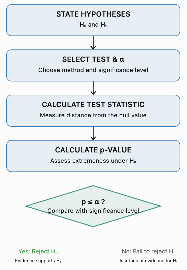
A hypothesis test generally involves five main steps:
-
State the null and alternative hypotheses.
-
Select an appropriate statistical test.
-
Calculate a test statistic.
-
Determine and interpret the p-value.
-
Make a statistical decision and explain the conclusion in context.
A successful hypothesis test requires both accurate calculations and careful interpretation. Statistical evidence is not the same as absolute proof.
What Is a Statistical Hypothesis?
A statistical hypothesis is a statement about a population parameter or probability distribution.
Common population parameters include:
-
μ: population mean.
-
p: population proportion.
-
μ₁ − μ₂: difference between two population means.
-
p₁ − p₂: difference between two population proportions.
Hypothesis testing uses sample statistics to evaluate these population claims.
For example, a school may want to determine whether the population mean test score is different from 70 marks.
The school collects a sample of test scores and evaluates whether the observed sample mean provides sufficient evidence of a difference.
The Null Hypothesis
The null hypothesis, written H₀, is the statement being tested.
In introductory tests, it commonly represents:
-
No change.
-
No difference.
-
No effect.
-
A specified population value.
Examples:
H₀: μ = 70
H₀: p = 0.50
H₀: μ₁ − μ₂ = 0
H₀: p₁ − p₂ = 0
The null hypothesis provides the reference model used to calculate how unusual the observed data would be.
The Alternative Hypothesis
The alternative hypothesis, written H₁ or Hₐ, describes the claim for which we seek evidence against H₀.
It may represent:
-
An increase.
-
A decrease.
-
A difference.
-
A nonzero effect.
Examples:
H₁: μ > 70
H₁: μ < 70
H₁: μ ≠ 70
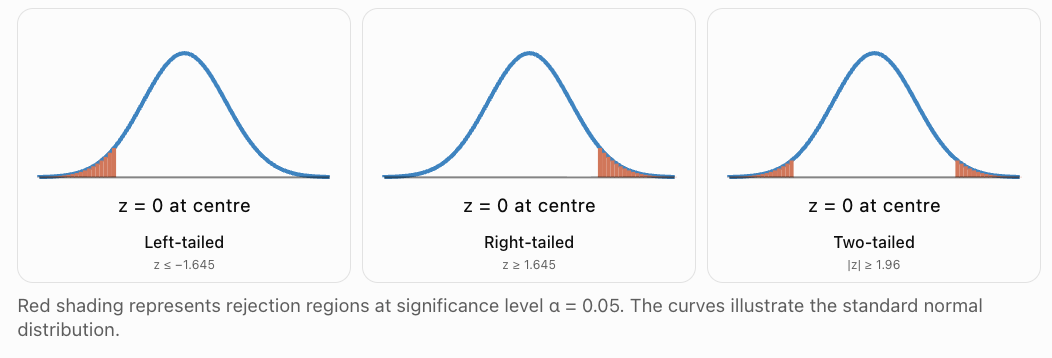
The alternative hypothesis determines whether the test is one-tailed or two-tailed.
One-Tailed and Two-Tailed Tests
Right-Tailed Test
A right-tailed test investigates whether a population parameter is greater than a specified value.
Example:
H₀: μ = 100
H₁: μ > 100
This test looks for unusually large sample results.
Left-Tailed Test
A left-tailed test investigates whether a population parameter is less than a specified value.
Example:
H₀: μ = 100
H₁: μ < 100
This test looks for unusually small sample results.
Two-Tailed Test
A two-tailed test investigates whether a population parameter differs from a specified value in either direction.
Example:
H₀: μ = 100
H₁: μ ≠ 100
Both unusually large and unusually small results can provide evidence against H₀.
Rejection regions for three types of z-test
Worked Example 1: Formulating Hypotheses
A company claims that the average mass of a cereal packet is 500 g.
A consumer group suspects that the packets are underfilled.
Step 1: Identify the parameter
Let μ be the population mean mass of all packets produced.
Step 2: Write the null hypothesis
H₀: μ = 500 g.
Step 3: Write the alternative hypothesis
H₁: μ < 500 g.
Step 4: Identify the test direction
The alternative hypothesis uses the less-than symbol.
Therefore, this is a left-tailed test.
The consumer group is seeking evidence that the mean packet mass is below 500 g.
Worked Example 2: Choosing a Two-Tailed Test
A school introduces a new teaching method and wants to investigate whether the mean mathematics score differs from the historical mean of 75 marks.
The school is interested in either improvement or decline.
Let μ be the population mean score under the new method.
H₀: μ = 75.
H₁: μ ≠ 75.
Answer: A two-tailed test.
The direction must be selected from the research question before examining the sample results. Choosing the direction after seeing the data can invalidate the reported p-value.
The Logic of Hypothesis Testing
Hypothesis testing begins by temporarily assuming that H₀ is true.
We then ask:
If H₀ were true, how unusual would the observed sample result be?
If the result is very unusual under H₀, it provides evidence against H₀.
If the result is not sufficiently unusual, we do not have enough evidence to reject H₀.
This does not establish that H₀ is true.
The General Process
The Significance Level
The significance level, written α (alpha), is the threshold used to decide whether a result is statistically significant.
Common choices are:
|
Significance level |
Percentage |
|---|---|
|
α = 0.10 |
10% |
|
α = 0.05 |
5% |
|
α = 0.01 |
1% |
The significance level should be chosen before examining the results.
At α = 0.05:
-
If p ≤ 0.05, reject H₀.
-
If p > 0.05, fail to reject H₀.
The value α represents the maximum probability of a Type I error under the test's null model and assumptions.
A smaller α requires stronger evidence before rejecting H₀.
Calculating Test Statistics
A test statistic measures how far a sample result is from the value predicted by H₀, relative to the sampling variability expected under H₀.
A general structure is:
Test statistic = (Observed estimate − Null value) / Standard error
A large absolute test statistic indicates that the observed result is far from the null value relative to its standard error.
Different hypothesis tests use different test statistics.
z-Test for a Population Mean
When the population standard deviation σ is known, a one-sample z-test may be appropriate.
Formula:
z = (x̄ − μ₀)/(σ/√n)
Where:
-
x̄ = sample mean.
-
μ₀ = population mean specified by H₀.
-
σ = known population standard deviation.
-
n = sample size.
The test assumes an appropriate random and independent sampling process and a normal or approximately normal sampling distribution of the mean.
Worked Example 3: Calculating a z-Test Statistic
A factory claims that the mean lifetime of its batteries is 500 hours.
A random sample of 64 batteries has:
x̄ = 485 hours.
σ = 40 hours.
Test whether the population mean is less than 500 hours.
Step 1: State the hypotheses
H₀: μ = 500.
H₁: μ < 500.
Step 2: Identify the information
x̄ = 485.
μ₀ = 500.
σ = 40.
n = 64.
Step 3: Calculate the standard error
SE = σ/√n
= 40/√64
= 40/8
= 5 hours.
Step 4: Calculate z
z = (485 − 500)/5
= −15/5
= −3.00.
Answer: z = −3.00.
The sample mean is three standard errors below the null-hypothesis mean.
A z-value of −3 is unusually low under the standard normal distribution.
The Standard Normal Distribution
Under H₀ and the z-test assumptions, the z-statistic follows a standard normal distribution, exactly or approximately.
The standard normal distribution has:
Mean = 0.
Standard deviation = 1.
Its shape is symmetric and bell-shaped.
Values close to zero are common, while values far from zero are less common.
The p-value is calculated from the appropriate tail area or areas of this distribution.
Understanding p-Values
The p-value is the probability, assuming the null hypothesis and the statistical model are correct, of obtaining a test statistic at least as extreme as the one observed, in the direction or directions specified by the alternative hypothesis.
A small p-value means that the observed result would be relatively unusual under H₀.
A large p-value means that the result is not particularly unusual under H₀.
Importantly:
-
A p-value is not the probability that H₀ is true.
-
A p-value is not the probability that the results occurred purely by chance.
-
A small p-value does not measure the size or practical importance of an effect.
-
A large p-value does not prove that H₀ is true.
Calculating p-Values from z-Statistics
Let Φ(z) represent the cumulative probability to the left of z under the standard normal distribution.
|
Alternative hypothesis |
p-value |
|---|---|
|
H₁: μ < μ₀ |
Φ(z) |
|
H₁: μ > μ₀ |
1 − Φ(z) |
|
H₁: μ ≠ μ₀ |
2Φ(−|z|) |
For a two-tailed test, the probability is calculated using both tails.
Worked Example 4: Completing the Battery Hypothesis Test
Return to the battery investigation.
H₀: μ = 500 hours.
H₁: μ < 500 hours.
Calculated test statistic:
z = −3.00.
Use α = 0.05.
Step 1: Calculate the p-value
Because this is a left-tailed test:
p = P(Z ≤ −3.00)
≈ 0.00135.
Step 2: Compare with α
0.00135 < 0.05.
Therefore, reject H₀.
Step 3: State the conclusion
There is statistically significant evidence at the 5% significance level that the population mean battery lifetime is less than 500 hours.
Step 4: Interpret the p-value
If the population mean really were 500 hours and the model assumptions held, the probability of obtaining a sample mean of 485 hours or less from a sample of 64 batteries would be approximately 0.135%.
This is strong evidence against the manufacturer's claimed mean.
It does not prove that every battery lasts less than 500 hours.
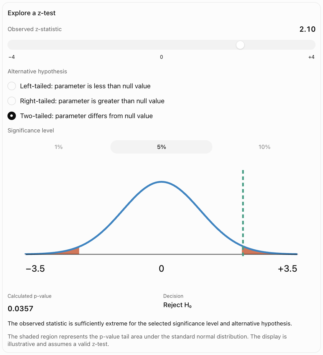
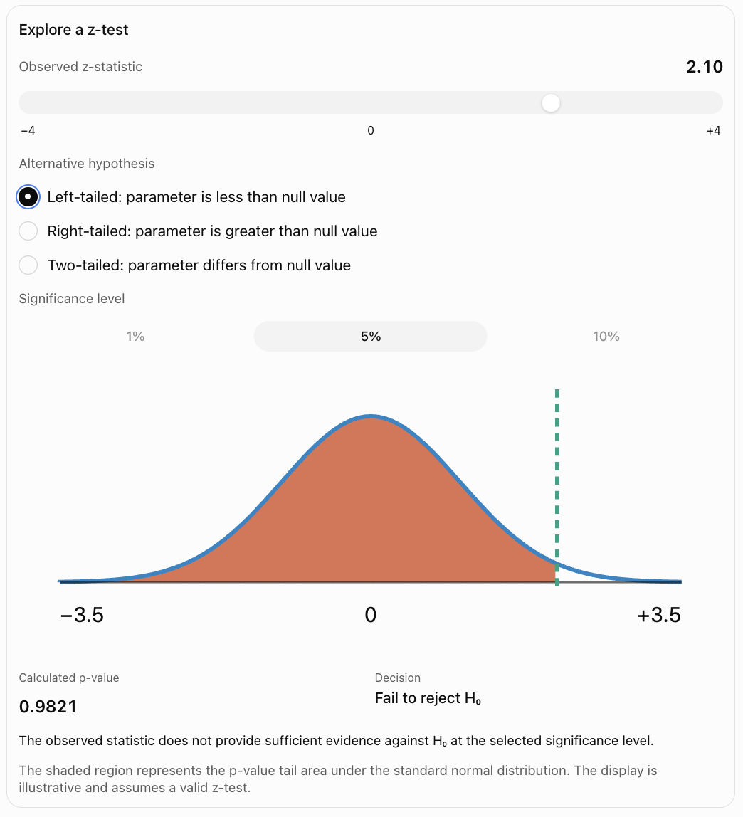
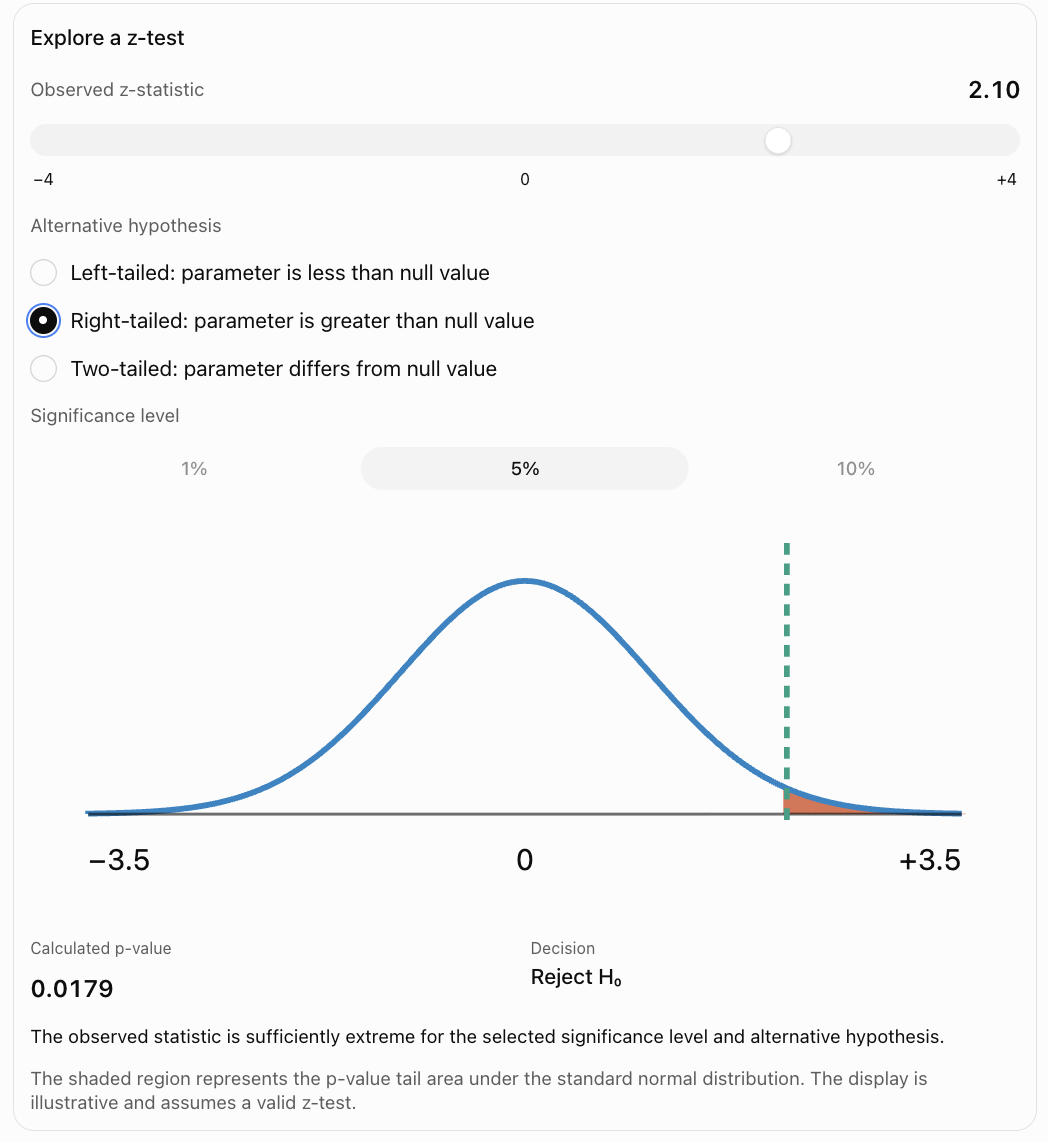
Interactive Hypothesis-Test Explorer
Use the controls to explore how the test statistic, alternative hypothesis, and significance level affect the statistical decision.
Worked Example 5: A Right-Tailed z-Test
A company claims that the mean delivery time is 30 minutes.
A random sample of 100 deliveries gives:
x̄ = 32.4 minutes.
The known population standard deviation is:
σ = 10 minutes.
Test whether the mean delivery time exceeds 30 minutes at α = 0.05.
Step 1: Hypotheses
H₀: μ = 30.
H₁: μ > 30.
Step 2: Standard error
SE = 10/√100 = 1.
Step 3: Test statistic
z = (32.4 − 30)/1
= 2.40.
Step 4: p-value
p = P(Z ≥ 2.40)
≈ 0.0082.
Step 5: Decision
0.0082 < 0.05.
Reject H₀.
Conclusion: There is statistically significant evidence that the population mean delivery time exceeds 30 minutes.
The sample mean suggests an increase of 2.4 minutes. Whether this increase is practically important depends on the business context.
Worked Example 6: A Two-Tailed z-Test
A filling machine is designed to dispense a mean of 250 mL.
A sample of 64 containers has:
x̄ = 247 mL.
σ = 12 mL.
Test whether the mean filling volume differs from 250 mL at α = 0.05.
Step 1: Hypotheses
H₀: μ = 250.
H₁: μ ≠ 250.
Step 2: Standard error
SE = 12/√64
= 1.5 mL.
Step 3: Test statistic
z = (247 − 250)/1.5
= −2.00.
Step 4: Two-tailed p-value
p = 2P(Z ≤ −2.00)
≈ 2(0.02275)
≈ 0.0455.
Step 5: Decision
0.0455 < 0.05.
Reject H₀.
Conclusion: There is statistically significant evidence that the population mean filling volume differs from 250 mL.
The sample indicates that the mean may be lower than the target.
Because this was a two-tailed test, the p-value includes extreme results in both directions.
t-Tests for a Population Mean
In many investigations, the population standard deviation σ is unknown.
Instead, the sample standard deviation s is used.
For a one-sample mean test, the appropriate statistic is usually:
t = (x̄ − μ₀)/(s/√n)
The degrees of freedom are:
df = n − 1
The p-value is calculated using Student's t-distribution.
A t-test requires an appropriate sampling design and distributional conditions. For small samples, the observations should be approximately normally distributed without severe outliers; larger samples allow more flexibility.
Worked Example 7: One-Sample t-Test
A school believes that the population mean mathematics test score is 70 marks.
A random sample of 25 students produces:
x̄ = 74.
s = 10.
Test whether the population mean score is different from 70 at α = 0.05.
Assume the t-test conditions hold.
Step 1: Hypotheses
H₀: μ = 70.
H₁: μ ≠ 70.
Step 2: Degrees of freedom
df = 25 − 1 = 24.
Step 3: Standard error
SE = 10/√25
= 2.
Step 4: Test statistic
t = (74 − 70)/2
= 2.00.
Step 5: p-value
For t = 2.00 with 24 degrees of freedom, using a two-tailed test:
p ≈ 0.057.
Step 6: Decision
0.057 > 0.05.
Fail to reject H₀.
Conclusion: There is insufficient statistical evidence at the 5% significance level that the population mean mathematics score differs from 70 marks.
This does not prove that the population mean is exactly 70.
The result is close to the significance threshold, illustrating why reporting the actual p-value is more informative than reporting only the decision.
Worked Example 8: A Left-Tailed t-Test
A factory claims that its components have a mean breaking strength of 100 N.
A random sample of 16 components has:
x̄ = 94 N.
s = 12 N.
Test whether the population mean breaking strength is less than 100 N.
Assume the population distribution is approximately normal.
Use α = 0.05.
Step 1: Hypotheses
H₀: μ = 100.
H₁: μ < 100.
Step 2: Degrees of freedom
df = 15.
Step 3: Standard error
SE = 12/√16 = 3 N.
Step 4: Test statistic
t = (94 − 100)/3
= −2.00.
Step 5: p-value
For t = −2.00 with df = 15, left-tailed:
p ≈ 0.032.
Step 6: Decision
0.032 < 0.05.
Reject H₀.
Conclusion: There is statistically significant evidence that the population mean breaking strength is below 100 N.
This may justify further quality-control investigation.
Hypothesis Tests for Population Proportions
Hypothesis tests are also used to investigate population proportions.
Examples include the proportion of students who prefer a new timetable, the percentage of defective products, and the proportion of households using renewable energy.
The sample proportion is:
p̂ = x/n
Where x is the number of observations with the characteristic and n is the sample size.
For a one-sample proportion z-test:
z = (p̂ − p₀)/√(p₀(1 − p₀)/n)
Where p₀ is the population proportion specified by H₀.
Notice that the standard error uses p₀, not p̂. This is because the test statistic is calculated under the null hypothesis.
For the normal approximation, common conditions include:
n p₀ ≥ 10
and
n(1 − p₀) ≥ 10.
The observations should also be independent or approximately independent, and the sampling design should be appropriate.
Worked Example 9: Testing a Population Proportion
A school claims that 50% of students prefer digital textbooks.
A random sample of 200 students finds that 120 prefer digital textbooks.
Test whether the population proportion is greater than 50% at α = 0.05.
Step 1: Hypotheses
H₀: p = 0.50.
H₁: p > 0.50.
Step 2: Calculate the sample proportion
p̂ = 120/200
= 0.60.
Step 3: Check the approximation
n p₀ = 200 × 0.50 = 100.
n(1 − p₀) = 100.
Both exceed 10.
Step 4: Calculate standard error under H₀
SE₀ = √(0.50 × 0.50/200)
= √0.00125
≈ 0.03536.
Step 5: Calculate the test statistic
z = (0.60 − 0.50)/0.03536
≈ 2.83.
Step 6: Calculate the p-value
This is a right-tailed test.
p = P(Z ≥ 2.83)
≈ 0.0023.
Step 7: Decision
0.0023 < 0.05.
Reject H₀.
Conclusion: There is statistically significant evidence that more than 50% of students in the population prefer digital textbooks.
Worked Example 10: Testing a Defect Rate
A manufacturer claims that 5% of its products are defective.
A random sample of 400 products contains 30 defective items.
Test whether the population defect rate exceeds 5% at α = 0.05.
Step 1: Hypotheses
H₀: p = 0.05.
H₁: p > 0.05.
Step 2: Sample proportion
p̂ = 30/400
= 0.075.
Step 3: Check conditions
n p₀ = 400 × 0.05 = 20.
n(1 − p₀) = 380.
The normal approximation is reasonable.
Step 4: Standard error
SE₀ = √(0.05 × 0.95/400)
≈ 0.01090.
Step 5: Test statistic
z = (0.075 − 0.05)/0.01090
≈ 2.29.
Step 6: p-value
p ≈ 0.0109.
Step 7: Decision
0.0109 < 0.05.
Reject H₀.
Conclusion: There is statistically significant evidence that the population defect rate exceeds 5%.
This finding could motivate further inspection of the manufacturing process.
Making Statistical Decisions
Once the p-value has been calculated, compare it with the chosen significance level.
|
Comparison |
Decision |
Meaning |
|---|---|---|
|
p ≤ α |
Reject H₀ |
Sufficient statistical evidence against H₀ |
|
p > α |
Fail to reject H₀ |
Insufficient statistical evidence against H₀ |
We generally avoid saying accept H₀.
A failure to reject may occur because the null hypothesis is correct, because the sample is too small, or because the true effect is difficult to detect.
Worked Example 11: Different Significance Levels
A hypothesis test produces:
p = 0.032.
Determine the decision at three significance levels.
|
Significance level |
Comparison |
Decision |
|---|---|---|
|
α = 0.10 |
0.032 < 0.10 |
Reject H₀ |
|
α = 0.05 |
0.032 < 0.05 |
Reject H₀ |
|
α = 0.01 |
0.032 > 0.01 |
Fail to reject H₀ |
The data and p-value have not changed.
Only the decision threshold has changed.
This demonstrates why a statistical report should include the p-value and the chosen significance level rather than simply stating that a result is significant.
Type I and Type II Errors
Hypothesis testing involves the possibility of incorrect decisions.
Type I Error
A Type I error occurs when H₀ is rejected even though it is true.
This is sometimes called a false positive.
The probability of a Type I error is controlled by the significance level α, under the test assumptions.
Type II Error
A Type II error occurs when H₀ is not rejected even though a particular alternative is true.
This is sometimes called a false negative.
The probability of a Type II error is represented by β (beta), for a specified alternative.
|
Reality |
Reject H₀ |
Fail to reject H₀ |
|---|---|---|
|
H₀ is true |
Type I error |
Correct decision |
|
H₀ is false |
Correct rejection |
Type II error |
Statistical Power
The power of a test is the probability of rejecting H₀ when a specified alternative is true.
Power = 1 − β
Higher power means a greater chance of detecting a real effect of the specified size.
Power is affected by:
-
Sample size.
-
Effect size.
-
Population variability.
-
Significance level.
-
Choice of statistical test.
Larger samples generally increase power when other conditions remain unchanged.
Worked Example 12: Understanding Errors in Context
A company tests whether its mean product mass is below the advertised 500 g.
H₀: μ = 500.
H₁: μ < 500.
A Type I error would occur if the company concluded that the population mean was below 500 g when the null value of 500 g was actually correct.
A Type II error would occur if the company failed to detect an actual reduction in mean mass.
The consequences differ.
A Type I error could cause unnecessary investigations or production changes.
A Type II error could allow an underfilling problem to continue.
The appropriate significance level should reflect the consequences of these errors, not merely a conventional choice of 0.05.
Statistical Significance Versus Practical Significance
A statistically significant result is not necessarily important in real life.
Suppose a very large sample finds that a new teaching method increases the mean test score by 0.2 marks.
The result might have a very small p-value because the estimate is extremely precise.
However, an increase of only 0.2 marks may have little practical educational value.
Conversely, a small study might estimate a substantial improvement but fail to reach statistical significance because the estimate is too uncertain.
Worked Example 13: A Large Sample with a Small Effect
A process has a historical mean output of 100 units.
A sample of 10,000 observations produces:
x̄ = 100.5.
Known σ = 10.
Test:
H₀: μ = 100.
H₁: μ ≠ 100.
Step 1: Standard error
SE = 10/√10000
= 0.1.
Step 2: Test statistic
z = (100.5 − 100)/0.1
= 5.00.
Step 3: p-value
The two-tailed p-value is approximately:
p ≈ 0.00000057.
This is statistically significant at α = 0.05.
However, the estimated increase is only 0.5 units, or 0.5% of the historical mean.
Conclusion: The data provide strong statistical evidence of a difference, but the practical importance of that difference must be evaluated separately.
Connecting Hypothesis Tests and Confidence Intervals
Hypothesis testing and confidence intervals are closely related.
For many standard two-sided tests, a hypothesis test at significance level α corresponds to a confidence interval with confidence level:
100(1 − α)%
For example:
A two-sided test at α = 0.05 corresponds to a 95% confidence interval when the test and interval use matching methods and assumptions.
If the null-hypothesis value lies outside the confidence interval, reject H₀.
If the null-hypothesis value lies inside the interval, fail to reject H₀.
This correspondence applies to compatible two-sided procedures; it should not be applied indiscriminately to one-sided tests or intervals constructed using different methods.
Worked Example 14: Testing with a Confidence Interval
A sample gives:
x̄ = 52.
Known σ = 12.
n = 36.
Test:
H₀: μ = 48.
H₁: μ ≠ 48.
Use α = 0.05.
Step 1: Calculate the standard error
SE = 12/√36
= 2.
Step 2: Construct the 95% confidence interval
CI = 52 ± 1.96 × 2
= 52 ± 3.92.
CI = (48.08, 55.92).
Step 3: Compare the null value
The null value is 48.
Since 48 lies outside the interval, reject H₀.
Step 4: Check with a test statistic
z = (52 − 48)/2
= 2.00.
Two-tailed p ≈ 0.0455.
Since p < 0.05, reject H₀.
Conclusion: Both methods agree that there is statistically significant evidence that the population mean differs from 48.
The confidence interval also provides a range of plausible values for the population mean, making it especially useful for communicating the size and uncertainty of the estimated effect.
Choosing the Appropriate Hypothesis Test
The correct test depends on the type of data, the parameter being investigated, and the study design.
|
Research question |
Common statistical test |
|---|---|
|
Is a population mean different from a specified value, with σ known? |
One-sample z-test |
|
Is a population mean different from a specified value, with σ unknown? |
One-sample t-test |
|
Is a population proportion different from a specified value? |
One-proportion z-test |
|
Do two independent population means differ? |
Two-sample t-test |
|
Is the mean difference between paired measurements zero? |
Paired t-test |
|
Do two population proportions differ? |
Two-proportion z-test |
|
Are two categorical variables associated? |
Chi-square test of independence |
Each test has assumptions that must be checked.
For example, a paired t-test is appropriate when the same students are measured before and after an intervention, while a two-sample t-test may be appropriate when comparing independent groups of students.
Worked Example 15: Paired Data
Ten students complete a mathematics assessment before and after a teaching intervention.
For each student, calculate:
Difference = After score − Before score.
The ten differences have:
Mean difference d̄ = 4.5 marks.
Standard deviation of differences s_d = 5 marks.
Test whether the mean improvement is greater than zero.
Assume the differences are approximately normally distributed and students are independently sampled.
Step 1: Hypotheses
Let μ_d be the population mean score difference.
H₀: μ_d = 0.
H₁: μ_d > 0.
Step 2: Standard error
SE = s_d/√n
= 5/√10
≈ 1.581.
Step 3: Test statistic
t = 4.5/1.581
≈ 2.846.
Step 4: Degrees of freedom
df = 10 − 1 = 9.
Step 5: p-value
For a right-tailed test:
p ≈ 0.0096.
Step 6: Decision
0.0096 < 0.05.
Reject H₀.
Conclusion: There is statistically significant evidence that the population mean after-minus-before score difference is positive.
However, without an appropriate comparison group, the improvement cannot automatically be attributed entirely to the teaching intervention. Other influences may have affected the scores.
Communicating the Conclusions of Hypothesis Tests
A complete statistical conclusion should contain four elements:
-
The statistical decision.
-
The significance level.
-
The population parameter and direction of the claim.
-
The strength and limitations of the evidence.
Example: Rejecting H₀
"At the 5% significance level, the test provides statistically significant evidence that the population mean battery lifetime is less than 500 hours (z = −3.00, p ≈ 0.00135)."
Example: Failing to Reject H₀
"At the 5% significance level, there is insufficient statistical evidence that the population mean test score differs from 70 marks (t = 2.00, df = 24, p ≈ 0.057)."
Avoid These Statements
Incorrect: "The null hypothesis is definitely false."
A hypothesis test provides evidence, not certainty.
Incorrect: "The null hypothesis is true because p > 0.05."
Failure to reject H₀ does not establish that H₀ is true.
Incorrect: "There is a 3% chance that the null hypothesis is true."
A p-value of 0.03 does not represent the probability that H₀ is true.
Incorrect: "The result is important because p < 0.05."
Statistical significance does not automatically establish practical importance.
Evaluating the Reliability of a Hypothesis Test
Before accepting a statistical conclusion, consider:
Sampling: Was the sample randomly selected and representative?
Independence: Are the observations independent, or was dependence properly modelled?
Distribution: Are the assumptions of the selected test reasonable?
Sample size: Is the sample large enough to provide useful power and support any approximations?
Measurement: Were the data collected accurately?
Effect size: How large is the observed difference?
Multiple testing: Were many hypotheses tested, increasing the chance of false positives?
Study design: Does the study support a causal conclusion, or only an association?
A small p-value cannot compensate for a fundamentally flawed study design.
Real-World Applications
Scientific research
Researchers test whether experimental results provide evidence of changes, differences, or relationships.
Quality control
Manufacturers test whether production processes meet target values and defect-rate requirements.
Education
Schools investigate whether student achievement differs from benchmarks or changes after interventions.
Environmental science
Scientists test claims about pollution levels, environmental changes, and water quality.
Integrated Investigation: Does a New Study Programme Improve Results?
A school introduces an optional mathematics study programme.
Historically, the mean score on a standardized assessment is 70 marks.
A random sample of 36 participating students obtains:
x̄ = 75 marks.
s = 12 marks.
The school wants to determine whether the population mean score among programme participants exceeds 70 marks.
Assume the observations are independent and the t-test conditions are appropriate.
Step 1: State the Hypotheses
H₀: μ = 70.
H₁: μ > 70.
Step 2: Select the Test
The population standard deviation is unknown.
Therefore, use a one-sample t-test.
Step 3: Choose the Significance Level
α = 0.05.
Step 4: Calculate the Standard Error
SE = 12/√36
= 2 marks.
Step 5: Calculate the Test Statistic
t = (75 − 70)/2
= 2.50.
Step 6: Degrees of Freedom
df = 36 − 1 = 35.
Step 7: Calculate the p-Value
For t = 2.50, df = 35, right-tailed:
p ≈ 0.0086.
Step 8: Make the Decision
0.0086 < 0.05.
Reject H₀.
Step 9: Communicate the Conclusion
There is statistically significant evidence at the 5% significance level that the population mean score among students participating in the programme exceeds 70 marks.
Step 10: Evaluate the Investigation
This does not prove that the programme caused the higher scores.
Students who volunteered for the programme may already be more motivated or better prepared.
A stronger causal investigation would use random assignment to programme and comparison groups, with appropriate analysis of the resulting outcomes.
This example demonstrates how hypothesis testing combines mathematical calculation, statistical interpretation, and critical evaluation.
Common Mistakes
Mistake 1: Confusing H₀ and H₁
The null hypothesis specifies the reference claim. The alternative describes the effect or difference being investigated.
Mistake 2: Using Sample Statistics in Hypotheses
Hypotheses concern population parameters, such as μ or p, rather than observed sample values such as x̄ or p̂.
Mistake 3: Choosing the Test Direction After Seeing the Data
The alternative hypothesis should be determined from the research question before examining the results.
Mistake 4: Using a Two-Tailed p-Value for a One-Tailed Test
The p-value must correspond to the specified alternative hypothesis.
Mistake 5: Forgetting the Standard Error
A test statistic compares a difference with its expected sampling variability, not merely with the raw standard deviation.
Mistake 6: Using σ When It Is Unknown
For a one-sample mean test with unknown σ, the t-test is generally appropriate.
Mistake 7: Forgetting Degrees of Freedom
For a one-sample t-test, df = n − 1.
Mistake 8: Using p̂ Instead of p₀ in a One-Proportion z-Test Standard Error
The test statistic uses the standard error calculated under H₀.
Mistake 9: Misinterpreting the p-Value
The p-value is not the probability that H₀ is true.
Mistake 10: Saying "Accept H₀"
The standard conclusion is "fail to reject H₀" when the evidence is insufficient.
Mistake 11: Treating Statistical Significance as Proof
Even statistically significant findings can be affected by sampling error, bias, or incorrect assumptions.
Mistake 12: Confusing Statistical Significance with Practical Importance
A very small effect may be statistically significant in a large sample.
Mistake 13: Ignoring Type I and Type II Errors
Both false rejection and failure to detect a real effect have consequences.
Mistake 14: Ignoring Sampling Bias
A large biased sample does not automatically support valid population inference.
Mistake 15: Failing to Check Test Assumptions
Independence, distributional conditions, and sampling design matter.
Mistake 16: Assuming a Nonsignificant Result Proves No Effect
The test may have insufficient power to detect a real effect.
Mistake 17: Using Inappropriate Precision
Report calculated values to a sensible number of decimal places without rounding intermediate calculations excessively.
Mistake 18: Making a Causal Claim from an Observational Study
An association or statistically significant difference does not necessarily establish causation.
Mistake 19: Ignoring Multiple Comparisons
Testing many hypotheses without appropriate adjustment increases the chance of obtaining false-positive findings.
Mistake 20: Giving a Decision Without Context
A complete conclusion should explain what the evidence means for the population and research question.
Key Terms
-
Hypothesis Testing: A statistical procedure for evaluating a claim about a population.
-
Statistical Hypothesis: A statement about a population parameter or distribution.
-
Null Hypothesis (H₀): The reference hypothesis evaluated by a statistical test.
-
Alternative Hypothesis (H₁ or Hₐ): The competing claim for which evidence is sought.
-
Population Parameter: A numerical characteristic of a population.
-
Sample Statistic: A numerical characteristic calculated from sample data.
-
Test Statistic: A standardized or otherwise defined measure of evidence against H₀.
-
z-Test: A test using the standard normal distribution under appropriate assumptions.
-
t-Test: A test using Student's t-distribution.
-
One-Tailed Test: A test for an effect in a specified direction.
-
Left-Tailed Test: A test with a less-than alternative.
-
Right-Tailed Test: A test with a greater-than alternative.
-
Two-Tailed Test: A test for a difference in either direction.
-
Significance Level (α): The chosen threshold controlling the Type I error probability.
-
p-Value: The probability under H₀ of a test statistic at least as extreme as the observed one.
-
Statistical Significance: A result meeting the chosen criterion for rejecting H₀.
-
Standard Error: The standard deviation of a statistic's sampling distribution, or an estimate of it.
-
Critical Value: A cutoff defining a rejection region.
-
Rejection Region: Values of a test statistic that lead to rejection of H₀.
-
Degrees of Freedom: A parameter determining the relevant t-distribution.
-
Type I Error: Rejecting a true null hypothesis.
-
Type II Error: Failing to reject a false null hypothesis.
-
Statistical Power: The probability of rejecting H₀ under a specified alternative.
-
Effect Size: A measure of the magnitude of an effect or difference.
-
Practical Significance: The real-world importance of an effect.
-
Confidence Interval: An interval estimate with a specified long-run coverage rate.
-
Sampling Variability: Differences between statistics obtained from different samples.
-
Random Sampling: Selecting observations using a chance-based procedure.
-
Sampling Bias: Systematic distortion caused by an unrepresentative selection process.
-
Normal Approximation: Using a normal distribution to approximate a sampling distribution.
-
Paired t-Test: A t-test applied to differences between paired observations.
-
Two-Sample t-Test: A test comparing the means of two independent populations.
-
One-Proportion z-Test: A test evaluating a population proportion using a normal approximation.
-
Multiple Testing: Conducting several hypothesis tests, potentially increasing false-positive risk.
-
Statistical Inference: Drawing conclusions about populations using sample data.
Key Takeaways
-
Hypothesis testing evaluates claims about population parameters.
-
The null hypothesis provides the reference model.
-
The alternative hypothesis specifies the claim being investigated.
-
Tests may be left-tailed, right-tailed, or two-tailed.
-
The test direction should be selected before examining the data.
-
A test statistic measures the observed difference relative to sampling variability.
-
z-tests and t-tests are used under different conditions.
-
One-proportion z-tests use the null proportion when calculating standard error.
-
A p-value measures how extreme the observed statistic is under H₀.
-
A small p-value provides evidence against H₀.
-
The significance level establishes the rejection threshold.
-
When p ≤ α, reject H₀.
-
When p > α, fail to reject H₀.
-
Failing to reject H₀ does not prove H₀ true.
-
Type I errors involve rejecting true null hypotheses.
-
Type II errors involve failing to detect false null hypotheses.
-
Statistical power describes the probability of detecting a specified real effect.
-
Statistical significance and practical significance are different.
-
Confidence intervals and compatible two-sided hypothesis tests are closely connected.
-
A complete conclusion includes the decision, evidence, context, and limitations.
Check Your Understanding
Use α = 0.05 unless another significance level is stated. Show your calculations and explain your decisions in context.
Question 1: Formulating Hypotheses
A company claims that the mean mass of its cereal packets is 400 g.
A researcher suspects that the mean mass is lower.
State H₀ and H₁, and identify the test direction.
Question 2: Two-Tailed Hypotheses
A school wants to investigate whether its population mean mathematics score differs from 75 marks.
Write the hypotheses and explain why the test is two-tailed.
Question 3: Calculating a z-Statistic
A sample of 100 measurements has:
x̄ = 54.
μ₀ = 50.
σ = 20.
Calculate the z-test statistic.
Question 4: Left-Tailed z-Test
A random sample of 64 products has:
x̄ = 98 g.
μ₀ = 100 g.
σ = 8 g.
Test whether the population mean mass is below 100 g.
Use the standard normal distribution.
Question 5: Right-Tailed z-Test
A sample of 100 observations has:
x̄ = 105.
μ₀ = 100.
σ = 20.
Test whether the population mean exceeds 100.
Question 6: Interpreting a p-Value
A hypothesis test produces p = 0.018.
Explain what the p-value means and state the decision at α = 0.05.
Question 7: Different Significance Levels
A test produces p = 0.034.
Determine the decision at:
a) α = 0.10.
b) α = 0.05.
c) α = 0.01.
Question 8: One-Sample t-Test
A random sample of 16 students has:
x̄ = 78.
s = 8.
Test whether the population mean score exceeds 75.
Assume the t-test conditions hold.
Use the t-distribution with 15 degrees of freedom.
Question 9: Population Proportion
A random sample of 200 students finds that 130 prefer digital learning materials.
Test whether the population proportion exceeds 0.50.
Question 10: Defect Rate
A manufacturer claims that 10% of its products are defective.
A random sample of 300 products contains 42 defective products.
Test whether the population defect proportion exceeds 10%.
Question 11: Type I and Type II Errors
A researcher tests whether the population mean concentration of a pollutant exceeds a specified safety threshold.
Explain Type I and Type II errors in this context.
Question 12: Statistical Versus Practical Significance
A large study finds that a new educational intervention increases average test scores by 0.1 marks, with p = 0.001.
Explain the statistical conclusion and why the result may not be practically important.
Question 13: Confidence Interval Connection
A 95% confidence interval for a population mean is:
(48, 56).
For a compatible two-sided test at α = 0.05, determine whether to reject H₀ when:
a) μ₀ = 50.
b) μ₀ = 45.
Question 14: Identifying Flawed Reasoning
A student writes:
"Because p = 0.12, there is a 12% probability that the null hypothesis is true. Therefore, we should accept the null hypothesis."
Identify and correct the errors.
Question 15: Comprehensive Hypothesis Test
A school claims that the population mean time students spend completing a mathematics assessment is 60 minutes.
A random sample of 36 students gives:
x̄ = 64 minutes.
s = 12 minutes.
Assume the t-test conditions hold.
Test whether the population mean completion time differs from 60 minutes.
Use:
α = 0.05.
For 35 degrees of freedom, the two-tailed p-value for t = 2.00 is approximately 0.053.
Calculate and explain:
a) The hypotheses.
b) The appropriate test.
c) The standard error.
d) The test statistic.
e) The p-value.
f) The statistical decision.
g) The conclusion in context.
h) Two limitations of the investigation.
Fully Worked Answers
Answer 1: Formulating Hypotheses
Let μ be the population mean mass of cereal packets.
H₀: μ = 400 g.
H₁: μ < 400 g.
Answer: Left-tailed test, because the researcher suspects that the mean is below 400 g.
Answer 2: Two-Tailed Hypotheses
Let μ be the population mean mathematics score.
H₀: μ = 75.
H₁: μ ≠ 75.
Answer: Two-tailed test.
The school is interested in differences in either direction, not only higher or lower scores.
Answer 3: Calculating a z-Statistic
Given:
x̄ = 54.
μ₀ = 50.
σ = 20.
n = 100.
Step 1: Standard error
SE = 20/√100
= 2.
Step 2: z-statistic
z = (54 − 50)/2
= 2.00.
Answer: z = 2.00.
The sample mean is two standard errors above the null value.
Answer 4: Left-Tailed z-Test
Step 1: Hypotheses
H₀: μ = 100.
H₁: μ < 100.
Step 2: Standard error
SE = 8/√64
= 1 g.
Step 3: Test statistic
z = (98 − 100)/1
= −2.00.
Step 4: p-value
p = P(Z ≤ −2.00)
≈ 0.0228.
Step 5: Decision
0.0228 < 0.05.
Reject H₀.
Conclusion: There is statistically significant evidence that the population mean product mass is below 100 g.
Answer 5: Right-Tailed z-Test
Step 1: Hypotheses
H₀: μ = 100.
H₁: μ > 100.
Step 2: Standard error
SE = 20/√100
= 2.
Step 3: Test statistic
z = (105 − 100)/2
= 2.50.
Step 4: p-value
p = P(Z ≥ 2.50)
≈ 0.0062.
Step 5: Decision
0.0062 < 0.05.
Reject H₀.
Conclusion: There is statistically significant evidence that the population mean exceeds 100.
Answer 6: Interpreting a p-Value
p = 0.018.
This means that, assuming H₀ and the statistical model are correct, the probability of obtaining a test statistic at least as extreme as the observed one is 1.8%, in the direction or directions specified by H₁.
Since:
0.018 < 0.05,
reject H₀.
Answer: The result is statistically significant at the 5% level.
Answer 7: Different Significance Levels
p = 0.034.
a) α = 0.10
0.034 < 0.10.
Reject H₀.
b) α = 0.05
0.034 < 0.05.
Reject H₀.
c) α = 0.01
0.034 > 0.01.
Fail to reject H₀.
Conclusion: The decision depends on the significance threshold, even though the sample evidence remains unchanged.
Answer 8: One-Sample t-Test
Given:
x̄ = 78.
μ₀ = 75.
s = 8.
n = 16.
Step 1: Hypotheses
H₀: μ = 75.
H₁: μ > 75.
Step 2: Standard error
SE = 8/√16
= 2.
Step 3: Test statistic
t = (78 − 75)/2
= 1.50.
Step 4: Degrees of freedom
df = 15.
Step 5: p-value
For t = 1.50, df = 15, right-tailed:
p ≈ 0.077.
Step 6: Decision
0.077 > 0.05.
Fail to reject H₀.
Conclusion: There is insufficient statistical evidence that the population mean score exceeds 75 marks.
Answer 9: Population Proportion
Given:
x = 130.
n = 200.
Step 1: Hypotheses
H₀: p = 0.50.
H₁: p > 0.50.
Step 2: Sample proportion
p̂ = 130/200
= 0.65.
Step 3: Standard error
SE₀ = √(0.50 × 0.50/200)
≈ 0.03536.
Step 4: Test statistic
z = (0.65 − 0.50)/0.03536
≈ 4.24.
Step 5: p-value
The right-tailed p-value is approximately 0.000011.
Step 6: Decision
p < 0.05.
Reject H₀.
Conclusion: There is strong statistical evidence that more than 50% of students in the population prefer digital learning materials.
Answer 10: Defect Rate
Given:
x = 42.
n = 300.
Step 1: Hypotheses
H₀: p = 0.10.
H₁: p > 0.10.
Step 2: Sample proportion
p̂ = 42/300
= 0.14.
Step 3: Check approximation
n p₀ = 30.
n(1 − p₀) = 270.
Both exceed 10.
Step 4: Standard error
SE₀ = √(0.10 × 0.90/300)
= √0.0003
≈ 0.01732.
Step 5: Test statistic
z = (0.14 − 0.10)/0.01732
≈ 2.31.
Step 6: p-value
Right-tailed p ≈ 0.0105.
Step 7: Decision
0.0105 < 0.05.
Reject H₀.
Conclusion: There is statistically significant evidence that the population defect rate exceeds 10%.
Answer 11: Type I and Type II Errors
Suppose the hypotheses are:
H₀: μ = the safety threshold.
H₁: μ > the safety threshold.
Type I error: Concluding that the population mean pollutant concentration exceeds the threshold when the null value is actually correct.
This could lead to unnecessary warnings or interventions.
Type II error: Failing to detect that the population mean pollutant concentration exceeds the threshold when it actually does.
This could allow a genuine environmental problem to remain undetected.
Both errors matter, but their consequences may differ substantially.
Answer 12: Statistical Versus Practical Significance
Given:
p = 0.001.
Since:
0.001 < 0.05,
the result is statistically significant.
There is evidence that the intervention changes the population mean score, assuming the test and study design are valid.
However, the estimated increase is only 0.1 marks.
This may be too small to produce a meaningful educational benefit.
Conclusion: Statistical significance does not necessarily imply practical significance.
Answer 13: Confidence Interval Connection
95% CI = (48, 56).
Use a compatible two-sided test at α = 0.05.
a) μ₀ = 50
50 lies inside the interval.
Therefore:
Fail to reject H₀.
b) μ₀ = 45
45 lies outside the interval.
Therefore:
Reject H₀.
This illustrates the relationship between compatible two-sided hypothesis tests and confidence intervals.
Answer 14: Identifying Flawed Reasoning
The student's statement contains two errors.
Error 1: A p-value of 0.12 does not mean that H₀ has a 12% probability of being true.
It means that, assuming H₀ and the statistical model are correct, the probability of obtaining a result at least as extreme as the observed one is 12%.
Error 2: The correct decision is not to "accept H₀."
At α = 0.05:
0.12 > 0.05.
Therefore:
Fail to reject H₀.
There is insufficient evidence against the null hypothesis, but this does not establish that it is true.
Answer 15: Comprehensive Hypothesis Test
Given:
x̄ = 64 minutes.
μ₀ = 60 minutes.
s = 12 minutes.
n = 36.
α = 0.05.
a) Hypotheses
H₀: μ = 60.
H₁: μ ≠ 60.
The test is two-tailed because the question asks whether the population mean differs from 60 minutes.
b) Appropriate test
Use a one-sample t-test because the population standard deviation is unknown.
c) Standard error
SE = s/√n
= 12/√36
= 12/6
= 2 minutes.
Answer: SE = 2 minutes.
d) Test statistic
t = (64 − 60)/2
= 2.00.
Answer: t = 2.00.
e) p-value
Degrees of freedom:
df = 36 − 1 = 35.
Given:
Two-tailed p ≈ 0.053.
f) Statistical decision
0.053 > 0.05.
Fail to reject H₀.
g) Conclusion in context
At the 5% significance level, there is insufficient statistical evidence that the population mean mathematics assessment completion time differs from 60 minutes.
The sample mean is 64 minutes, but the observed difference is not statistically significant at the chosen threshold.
This does not prove that the true mean is exactly 60 minutes.
h) Two limitations
-
The sample may not fully represent the school population, especially if some student groups are underrepresented.
-
Completion times may be affected by differences in assessment difficulty, testing conditions, or student preparation.
A larger, representative sample and consistent testing conditions could improve the investigation.
Final Course Connections
Hypothesis testing connects probability distributions, sampling variability, standard errors, confidence intervals, and statistical inference.
It provides a structured way to evaluate claims using evidence rather than relying on individual observations or assumptions.
The essential process is to formulate appropriate hypotheses, select a valid statistical test, calculate the test statistic and p-value, make a decision using the significance level, and communicate the conclusion in the context of the original question.
The most important distinction is that hypothesis testing evaluates the strength of statistical evidence; it does not establish absolute certainty.
This completes Hypothesis Testing, covering all five learning targets with 15 worked examples, explanatory diagrams, an interactive z-test explorer, real-world applications, common mistakes, key terms, key takeaways, and 15 practice questions with fully worked answers.
3. Errors in Statistical Testing
Learning outcomes
- I can distinguish between Type I and Type II errors.
- I can explain statistical significance.
- I can interpret significance levels.
- I can evaluate statistical conclusions.
- I can explain limitations of hypothesis testing.
Introduction
Statistical hypothesis testing helps researchers make decisions using sample data. However, because samples contain uncertainty, statistical decisions can sometimes be wrong.
Imagine a medical screening test that indicates a person has a particular disease. The result could be correct, but it could also be a false positive. Alternatively, a screening test might fail to detect a disease that is actually present.
A similar problem occurs in statistical hypothesis testing.
A researcher may:
-
Reject a null hypothesis that is actually true.
-
Fail to reject a null hypothesis that is actually false.
These mistakes are known as Type I and Type II errors.
Understanding these errors is essential because statistical significance does not guarantee that a conclusion is correct, important, or reliable.
In this lesson, we will explore how errors occur, how significance levels influence decisions, how statistical power affects the detection of real effects, and why hypothesis tests must be interpreted carefully.
Review: The Logic of Hypothesis Testing
A hypothesis test evaluates a claim about a population parameter using sample data.
The two competing hypotheses are:
Null hypothesis (H₀): The reference claim being tested, often representing no difference or no effect.
Alternative hypothesis (H₁ or Hₐ): The competing claim that the researcher is investigating.
For example, a manufacturer claims that its batteries have a mean lifetime of 500 hours.
H₀: μ = 500 hours
H₁: μ < 500 hours
The researcher collects a sample and calculates a test statistic and p-value.
The decision depends on the significance level, α.
-
If p ≤ α, reject H₀.
-
If p > α, fail to reject H₀.
These decisions are made using incomplete information about the population. Therefore, mistakes are possible.
The Four Possible Outcomes
A hypothesis test can produce four combinations of reality and decision.
|
Actual situation |
Reject H₀ |
Fail to reject H₀ |
|---|---|---|
|
H₀ is true |
Type I error |
Correct decision |
|
H₀ is false |
Correct rejection |
Type II error |
This table is fundamental to understanding statistical errors.
There are two correct outcomes and two incorrect outcomes.
Importantly, in real investigations we generally do not know with certainty whether H₀ is true. The table describes possible outcomes, not information that the researcher necessarily possesses.
Type I Errors: False Positives
A Type I error occurs when we reject H₀ even though H₀ is true.
In simpler language:
We conclude that an effect or difference exists when the null hypothesis is actually true.
This is often described as a false positive.
Example: A Manufacturing Process
A factory produces components with a target mean mass of 200 g.
The hypotheses are:
H₀: μ = 200 g
H₁: μ ≠ 200 g
A Type I error occurs if the researcher concludes that the mean mass differs from 200 g when the true population mean is actually 200 g.
The factory might unnecessarily stop production, recalibrate machinery, or discard acceptable products.
Example: A New Teaching Method
A researcher investigates whether a new teaching method changes the population mean examination score.
H₀: μ_new − μ_old = 0
H₁: μ_new − μ_old ≠ 0
A Type I error occurs if the researcher concludes that the method changes scores when the true population mean difference is zero.
This could cause a school to adopt an intervention that does not actually improve average performance.
Probability of a Type I Error
The probability of a Type I error is represented by:
α (alpha)
For a test with a valid null model and a significance level of 0.05, the probability of incorrectly rejecting H₀ when H₀ is true is at most 5%.
In many continuous tests, it is exactly 5%.
This is why α is also called the significance level.
Type II Errors: False Negatives
A Type II error occurs when we fail to reject H₀ even though H₀ is false.
In simpler language:
A real effect or difference exists, but the test fails to detect it.
This is often described as a false negative.
Example: A Manufacturing Process
Suppose the true mean component mass has fallen to 195 g.
However, the sample results do not provide sufficient evidence to reject:
H₀: μ = 200 g.
The researcher fails to detect the actual change.
This is a Type II error.
Example: A New Teaching Method
Suppose a new teaching method genuinely increases the population mean score by 5 marks.
However, the study uses a small sample and obtains p = 0.12.
At α = 0.05, the researcher fails to reject H₀.
If the true mean difference is nonzero, this is a Type II error.
The researcher may incorrectly conclude that there is insufficient evidence to support adopting a genuinely beneficial intervention.
Notice the distinction: failing to reject H₀ is not automatically a Type II error. It is a Type II error only when H₀ is actually false.
Comparing Type I and Type II Errors
|
Feature |
Type I error |
Type II error |
|---|---|---|
|
Statistical decision |
Reject H₀ |
Fail to reject H₀ |
|
Reality |
H₀ is true |
H₀ is false |
|
Common description |
False positive |
False negative |
|
Probability |
α, or at most α |
β |
|
Main consequence |
Detecting a nonexistent effect |
Missing a real effect |
Worked Example 1: Identifying Errors in Context
A company tests whether the population mean concentration of a chemical in drinking water exceeds a safety limit of 10 mg/L.
For the test, use:
H₀: μ = 10 mg/L
H₁: μ > 10 mg/L
Situation A: The true mean concentration is 10 mg/L, but the test concludes that it is higher.
This is a Type I error.
Situation B: The true mean concentration is 12 mg/L, but the test fails to reject H₀.
This is a Type II error.
Situation C: The true mean concentration is 12 mg/L, and the test rejects H₀.
This is a correct rejection.
Situation D: The true mean concentration is 10 mg/L, and the test fails to reject H₀.
This is a correct decision.
In environmental monitoring, a Type II error could be especially serious because a genuine safety problem may go undetected.
In a real regulatory setting, the hypotheses and safety decision rules should be chosen to reflect which errors are most costly.
Statistical Significance
A result is statistically significant when the p-value is less than or equal to the chosen significance level.
For example, at α = 0.05:
-
p = 0.003 is statistically significant.
-
p = 0.041 is statistically significant.
-
p = 0.072 is not statistically significant.
-
p = 0.310 is not statistically significant.
Statistical significance means that the observed data are sufficiently incompatible with H₀, according to the selected test and threshold, to justify rejecting H₀.
It does not necessarily mean that the effect is large, important, or causal.
Understanding the p-Value
A p-value is the probability, assuming H₀ and the statistical model are correct, of obtaining a test statistic at least as extreme as the observed one in the direction or directions specified by H₁.
For example:
p = 0.02
means that, if H₀ and the model were correct, a result at least as extreme as the observed one would occur with probability 2%.
It does not mean:
-
There is a 2% probability that H₀ is true.
-
There is a 98% probability that H₁ is true.
-
The result has a 98% probability of being correct.
-
The effect is necessarily important.
Worked Example 2: Interpreting Statistical Significance
A school investigates whether the population mean test score differs from 70 marks.
H₀: μ = 70
H₁: μ ≠ 70
The test produces:
p = 0.032
At α = 0.05:
0.032 < 0.05
Therefore, reject H₀.
Conclusion: There is statistically significant evidence that the population mean test score differs from 70 marks.
However, the p-value does not tell us how large the difference is. We would need the estimated mean difference and preferably a confidence interval to evaluate its magnitude and precision.
Significance Levels and the Risk of Error
The significance level α is selected before examining the sample results.
It determines how much evidence is required before rejecting H₀.
Common choices include:
|
Significance level |
Interpretation under a true H₀ |
|---|---|
|
α = 0.10 |
Up to 10% probability of a Type I error |
|
α = 0.05 |
Up to 5% probability of a Type I error |
|
α = 0.01 |
Up to 1% probability of a Type I error |
A smaller significance level makes the test more conservative about rejecting H₀.
However, it does not automatically make the test better. A stricter threshold can make genuine effects harder to detect.
Worked Example 3: Different Significance Levels
A researcher obtains:
p = 0.028
Determine the decision at three significance levels.
At α = 0.10:
0.028 < 0.10
Reject H₀.
At α = 0.05:
0.028 < 0.05
Reject H₀.
At α = 0.01:
0.028 > 0.01
Fail to reject H₀.
The sample evidence has not changed. Only the decision threshold has changed.
This is why researchers should report the actual p-value rather than merely saying that a result is significant or not significant.
Critical Values and Rejection Regions
A significance level can also be expressed using critical values.
For a two-tailed z-test at α = 0.05, the critical values are:
z = −1.96 and z = +1.96.
Reject H₀ if:
z < −1.96 or z > +1.96.
Otherwise, fail to reject H₀.
Two-tailed z-test at α = 0.05
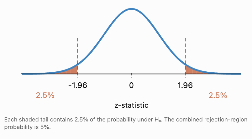
Worked Example 4: Using Critical Values
A two-tailed z-test produces:
z = 2.24.
The significance level is:
α = 0.05.
The critical values are ±1.96.
Since:
2.24 > 1.96,
the test statistic lies in the rejection region.
Decision: Reject H₀.
The corresponding two-tailed p-value is approximately 0.0251, which is also below 0.05.
Both approaches give the same decision.
Statistical Power and Type II Errors
The probability of a Type II error is represented by:
β (beta)
Statistical power is defined as:
Power = 1 − β
Power is the probability that a test correctly rejects H₀ when a specified alternative is true.
For example:
If β = 0.20,
Power = 1 − 0.20
= 0.80
= 80%.
This means that, if the specified alternative were true, the test would reject H₀ in approximately 80% of repeated studies.
The remaining 20% would result in Type II errors.
Unlike α, β is not usually a single fixed number for every false value of H₀. It depends on the actual effect size and other features of the study.
Factors Affecting Statistical Power
Power generally increases when:
-
Sample size increases.
-
The true effect is larger.
-
Population variability decreases.
-
The significance level is increased, all else equal.
-
The statistical design and measurement process become more efficient.
A test with low power may fail to detect effects that genuinely exist.
Worked Example 5: Calculating Power
A study has a Type II error probability of:
β = 0.15.
Calculate its power.
Power = 1 − β
= 1 − 0.15
= 0.85.
Answer: 85% power.
For the specified alternative, the test has an 85% probability of correctly rejecting H₀.
Worked Example 6: Understanding a Low-Power Study
A researcher investigates whether a new learning programme improves mean test scores.
The study has only eight participants and high variation in student performance.
The test produces:
p = 0.18.
At α = 0.05, the researcher fails to reject H₀.
Can the researcher conclude that the programme has no effect?
No.
The small sample and high variability may result in low statistical power.
A genuine improvement could exist but remain undetected.
A better conclusion is:
"There is insufficient evidence from this study to conclude that the programme improves mean test scores."
A larger, well-designed study could provide a more precise estimate.
The Trade-Off Between Type I and Type II Errors
When sample size and other study conditions remain fixed, lowering α generally reduces the probability of a Type I error but increases the probability of a Type II error for a specified alternative.
Consider a right-tailed z-test of:
H₀: μ = 100
H₁: μ > 100.
Suppose the standard error is 5.
The sample mean must exceed a critical value before H₀ is rejected.
At α = 0.10:
Critical z ≈ 1.282.
Critical sample mean:
100 + 1.282 × 5 = 106.41.
At α = 0.05:
Critical z ≈ 1.645.
Critical sample mean:
100 + 1.645 × 5 = 108.23.
At α = 0.01:
Critical z ≈ 2.326.
Critical sample mean:
100 + 2.326 × 5 = 111.63.
As α decreases, the sample mean must be larger before H₀ is rejected.
Interactive Example: Significance and Power
Suppose the true population mean is 110, the null mean is 100, and the standard error is 5. Explore the consequences of changing α for a right-tailed z-test.
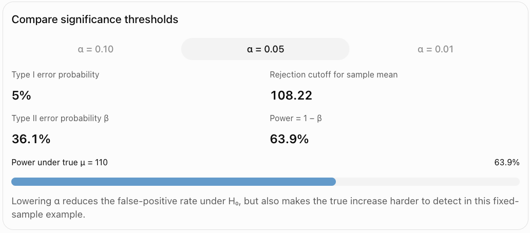
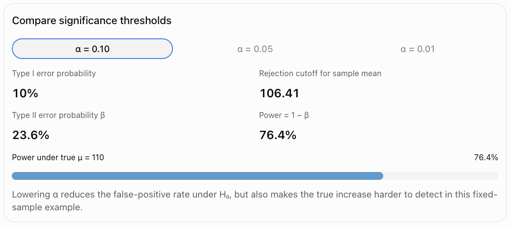
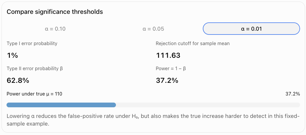
The trade-off can be improved by increasing sample size or reducing measurement variability, rather than simply changing α.
Calculating Type II Error Probability
To calculate β, we need to specify an actual alternative value of the population parameter.
Worked Example 7: Calculating β and Power
A factory tests whether the mean mass of a product exceeds 100 g.
Assume:
H₀: μ = 100 g
H₁: μ > 100 g
Known population standard deviation:
σ = 10 g.
Sample size:
n = 25.
Significance level:
α = 0.05.
Suppose the actual population mean is 105 g.
Calculate β and power.
Step 1: Standard error
SE = σ/√n
= 10/√25
= 2 g.
Step 2: Find the rejection cutoff
For a right-tailed test at α = 0.05:
z* = 1.645.
Reject H₀ when:
x̄ > 100 + 1.645(2)
x̄ > 103.29 g.
Step 3: Calculate β under the true mean of 105 g
A Type II error occurs when the test fails to reject H₀, so:
β = P(x̄ ≤ 103.29 | μ = 105).
Standardize:
z = (103.29 − 105)/2
= −0.855.
Therefore:
β = P(Z ≤ −0.855)
≈ 0.196.
Step 4: Calculate power
Power = 1 − 0.196
= 0.804.
Answer: β ≈ 19.6%, power ≈ 80.4%.
If the true population mean were 105 g, the test would detect the increase in approximately 80.4% of repeated samples.
Worked Example 8: Increasing Sample Size
Keep the same investigation, but increase the sample size from 25 to 100.
Now:
SE = 10/√100 = 1 g.
The rejection cutoff becomes:
100 + 1.645(1) = 101.645 g.
If the true mean is 105 g:
β = P(x̄ ≤ 101.645 | μ = 105).
Standardize:
z = (101.645 − 105)/1
= −3.355.
Thus:
β ≈ 0.0004.
Power ≈ 0.9996
≈ 99.96%.
Conclusion: Increasing sample size from 25 to 100 dramatically increases power to detect a true mean of 105 g, under the assumed model.
However, large sample sizes do not eliminate bias or guarantee practical importance.
Evaluating Statistical Conclusions
A statistical conclusion should be evaluated using more than its p-value.
Researchers should consider the estimated effect, uncertainty, study design, statistical assumptions, and real-world consequences.
Statistical Significance Versus Practical Significance
Statistical significance describes whether the data provide sufficient evidence against H₀ at the chosen α.
Practical significance describes whether the size of the effect matters in the real world.
Worked Example 9: A Statistically Significant but Small Effect
A manufacturer tests whether the mean diameter of a component differs from 20 mm.
A sample of 10,000 components produces:
x̄ = 20.02 mm.
Known σ = 0.5 mm.
H₀: μ = 20
H₁: μ ≠ 20.
Step 1: Standard error
SE = 0.5/√10000
= 0.005 mm.
Step 2: Test statistic
z = (20.02 − 20)/0.005
= 4.00.
Step 3: p-value
For a two-tailed test:
p ≈ 0.000063.
This is statistically significant at α = 0.05.
However, the estimated difference is only 0.02 mm.
Whether that difference matters depends on manufacturing tolerances.
Conclusion: The statistical evidence for a difference is strong, but the practical importance cannot be determined without the engineering requirements.
Confidence Intervals and Statistical Conclusions
Confidence intervals help evaluate the magnitude and precision of estimated effects.
For compatible two-sided procedures:
A 95% confidence interval corresponds to a hypothesis test at α = 0.05.
If the null value lies outside the interval, reject H₀.
If it lies inside the interval, fail to reject H₀.
Worked Example 10: Using a Confidence Interval
A study estimates a mean improvement of 3.5 marks.
The 95% confidence interval for the population mean improvement is:
(0.8, 6.2) marks.
Test:
H₀: μ_d = 0
H₁: μ_d ≠ 0.
Because zero is outside the interval, reject H₀ at α = 0.05, assuming the interval and test are compatible.
There is statistically significant evidence of a nonzero mean improvement.
However, the plausible improvement ranges from 0.8 to 6.2 marks.
If an improvement of at least 5 marks is required to justify the cost of the programme, the interval does not establish that the improvement meets that practical threshold.
Evaluating a Nonsignificant Result
A nonsignificant result does not establish that there is no effect.
Consider two studies.
Study A: Estimated effect = 0.2 marks, 95% CI = (−0.3, 0.7).
Study B: Estimated effect = 0.2 marks, 95% CI = (−8.0, 8.4).
Both intervals contain zero, so neither produces a significant result at the corresponding two-sided 5% level.
However, they tell different stories.
Study A estimates the effect relatively precisely and suggests that large effects are unlikely.
Study B is highly uncertain and remains compatible with both substantial harm and substantial benefit.
Therefore, absence of statistically significant evidence is not the same as evidence of absence.
To establish that an effect is small enough to be practically negligible, researchers may use equivalence tests with predefined equivalence margins.
Worked Example 11: Evaluating Two Studies
A researcher wants to know whether a new teaching programme changes mean test scores by at least 5 marks.
Two studies produce the following results:
|
Study A |
Study B |
|
|---|---|---|
|
Estimated change |
+1 mark |
+1 mark |
|
95% CI |
(0.2, 1.8) |
(−7, 9) |
|
Statistical significance versus zero |
Significant |
Not significant |
Study A: There is evidence of a positive mean change, but the entire confidence interval is below 5 marks. The estimated effect is unlikely to reach the practical target under the model.
Study B: There is insufficient evidence of a nonzero mean change, but the interval includes changes greater than 5 marks. The study is too imprecise to rule out a practically important improvement.
The two studies should not be described simply as one successful and one unsuccessful. Their estimates and uncertainties must be interpreted.
Limitations of Hypothesis Testing
Sampling Bias
If the sample does not represent the target population, statistical results may be misleading.
A small p-value cannot correct a biased sampling process.
Measurement Error
Poorly calibrated instruments, inaccurate self-reporting, or inconsistent procedures can distort results.
Violated Statistical Assumptions
Tests may require independent observations, particular distributional conditions, or sufficiently large samples.
Violating these assumptions can make p-values and error rates unreliable.
Low Statistical Power
A small study may fail to detect a real effect.
A nonsignificant result from a low-power study should be interpreted cautiously.
Multiple Hypothesis Testing
When many tests are performed, the probability of obtaining at least one false positive increases.
If 20 independent tests are performed at α = 0.05 and all null hypotheses are true, the probability of at least one false rejection is:
P(at least one false positive) = 1 − (1 − 0.05)²⁰
= 1 − 0.95²⁰
≈ 0.642.
Answer: Approximately 64.2%.
The calculation assumes independent tests. Dependence changes the exact probability, but multiple testing remains an important concern.
Methods such as the Bonferroni correction and false discovery rate procedures can help manage multiple-testing errors.
Selective Reporting
If researchers report only statistically significant results and omit nonsignificant findings, the published evidence may be distorted.
p-Hacking
Repeatedly changing analyses, excluding observations without a justified plan, or testing many alternatives until p < 0.05 can increase false-positive risk.
Confounding Variables
An observed association may be influenced by other variables.
For example, students who participate in optional tutoring may have higher scores because of differences in motivation or prior achievement.
A significant result alone does not establish causation.
Model Dependence
Statistical conclusions depend on the chosen model.
An incorrect model may produce misleading estimates and significance tests.
Generalizability
A result obtained from one group or setting may not apply to other populations.
Worked Example 12: Multiple Testing
A researcher tests 20 unrelated outcomes at α = 0.05.
Assume all 20 null hypotheses are true and the tests are independent.
The probability that none produces a Type I error is:
0.95²⁰ ≈ 0.3585.
Therefore, the probability of at least one false positive is:
1 − 0.3585
≈ 0.6415.
Answer: Approximately 64.2%.
This does not mean that 64.2% of the tests will be false positives. It means that the probability of getting at least one false positive across the 20 tests is approximately 64.2%.
Real-World Applications
Medical research
Researchers balance the risks of falsely detecting treatment effects and failing to detect genuine benefits or harms.
Manufacturing
Quality-control decisions balance unnecessary production interruptions against missed defects.
Education
Schools evaluate interventions while considering sample size, uncertainty, and practical improvements.
Environmental monitoring
Statistical testing helps identify changes in environmental conditions, while missed problems may have serious consequences.
Integrated Investigation: Evaluating a New Teaching Programme
A school wants to determine whether a new mathematics programme improves average test scores.
The historical mean score is 70 marks.
A random sample of 36 students enrolled in the programme has:
x̄ = 74 marks
s = 12 marks.
Assume a one-sample t-test is appropriate.
Step 1: Hypotheses
H₀: μ = 70
H₁: μ > 70.
Step 2: Significance Level
α = 0.05.
Step 3: Standard Error
SE = 12/√36
= 2 marks.
Step 4: Test Statistic
t = (74 − 70)/2
= 2.00.
Degrees of freedom:
df = 35.
Step 5: p-Value
For a right-tailed t-test with t = 2.00 and df = 35:
p ≈ 0.0266.
Step 6: Statistical Decision
0.0266 < 0.05.
Reject H₀.
Step 7: Statistical Conclusion
There is statistically significant evidence at the 5% level that the population mean score among students enrolled in the programme exceeds 70 marks.
Step 8: Possible Errors
Type I error: Concluding that the population mean score exceeds 70 when it is actually 70.
Type II error: Failing to detect a genuine increase above 70. This study rejected H₀, so a Type II error was not the decision made.
Step 9: Evaluate the Conclusion
The result is statistically significant, but several questions remain:
-
Were the students representative of the target population?
-
Did students volunteer for the programme?
-
Were the tests comparable to the historical assessments?
-
Was the estimated improvement large enough to justify the programme's cost?
-
Could other changes explain the higher scores?
Without random assignment or another credible causal design, the test does not prove that the programme caused the improvement.
Overall conclusion: The evidence suggests a higher population mean score among programme participants, but the causal and practical conclusions require additional investigation.
Common Mistakes
-
Confusing Type I and Type II errors: Type I means rejecting a true H₀; Type II means failing to reject a false H₀.
-
Assuming a rejected H₀ must be false: A Type I error remains possible.
-
Assuming failure to reject proves H₀: The test may lack sufficient power.
-
Interpreting α as the probability that H₀ is true: α controls the false-rejection probability under H₀.
-
Assuming β always equals 1 − α: β depends on the alternative, sample size, variability, and test.
-
Confusing statistical significance with practical importance: A tiny effect can be statistically significant.
-
Interpreting p = 0.03 as a 3% probability that H₀ is true: This is not the meaning of a p-value.
-
Changing α after examining results: This undermines the integrity of the decision procedure.
-
Assuming a larger α is always better: It generally increases power but also increases Type I error risk.
-
Assuming a smaller α eliminates errors: It reduces false-positive risk but can increase false negatives.
-
Ignoring sample size: Small samples may have low power.
-
Ignoring effect size: The magnitude of a difference matters.
-
Ignoring confidence intervals: A p-value alone does not adequately communicate precision.
-
Treating a nonsignificant result as proof of equivalence: Equivalence requires an appropriate design and test.
-
Assuming large samples eliminate bias: A large biased sample can produce misleading results.
-
Ignoring multiple comparisons: Repeated testing increases the opportunity for false-positive findings.
-
Assuming statistical significance establishes causation: Confounding and selection bias may explain associations.
-
Overlooking assumptions: Incorrect assumptions can invalidate nominal error rates.
-
Reporting only significant findings: Selective reporting distorts the evidence.
-
Using absolute language: Statistical conclusions should acknowledge uncertainty and limitations.
Key Terms
-
Hypothesis Test: A statistical procedure for evaluating a claim about a population.
-
Null Hypothesis (H₀): The reference hypothesis tested against the data.
-
Alternative Hypothesis (H₁): The competing claim for which evidence is sought.
-
Type I Error: Rejecting H₀ when H₀ is true.
-
Type II Error: Failing to reject H₀ when H₀ is false.
-
False Positive: A positive conclusion when the tested null condition is actually true.
-
False Negative: A failure to detect an effect that genuinely exists.
-
Significance Level (α): The selected upper bound on the Type I error probability.
-
Beta (β): The Type II error probability under a specified alternative.
-
Statistical Power: The probability of correctly rejecting H₀ under a specified alternative.
-
p-Value: The probability, under H₀ and the model, of a test statistic at least as extreme as the observed one.
-
Statistical Significance: Meeting the chosen criterion for rejecting H₀.
-
Practical Significance: The real-world importance of an estimated effect.
-
Effect Size: A numerical measure of the magnitude of an effect.
-
Test Statistic: A value summarizing how strongly the sample conflicts with H₀.
-
Critical Value: A cutoff used to define a rejection region.
-
Rejection Region: Test-statistic values that lead to rejection of H₀.
-
Standard Error: A measure of the sampling variability of a statistic.
-
Confidence Interval: An interval estimate constructed using a procedure with a specified coverage rate.
-
Sampling Variability: Natural differences between statistics from different samples.
-
Sampling Bias: Systematic distortion caused by an unrepresentative sampling process.
-
Measurement Error: Inaccuracy in observed or recorded values.
-
Confounding Variable: A variable that distorts an apparent relationship between other variables.
-
Multiple Testing: Conducting several statistical tests within an investigation.
-
Familywise Error Rate: The probability of making at least one Type I error across a family of tests.
-
Bonferroni Correction: A method for controlling familywise error by adjusting individual test thresholds.
-
False Discovery Rate: The expected proportion of false rejections among rejected hypotheses, under the relevant procedure's conditions.
-
p-Hacking: Manipulating or selectively exploring analyses to obtain significant results.
-
Selective Reporting: Reporting results based on whether they support a preferred conclusion.
-
Equivalence Testing: Testing whether an effect lies within predefined practically negligible bounds.
-
Generalizability: The extent to which study conclusions apply to a wider population.
-
Statistical Assumption: A condition required for a method's validity.
Key Takeaways
-
Hypothesis tests can produce correct or incorrect decisions.
-
A Type I error occurs when a true null hypothesis is rejected.
-
A Type II error occurs when a false null hypothesis is not rejected.
-
The significance level α controls the Type I error risk under the null model.
-
The probability β measures Type II error risk for a specified alternative.
-
Statistical power equals 1 − β.
-
Increasing sample size generally improves power.
-
Lowering α generally reduces Type I errors but can increase Type II errors.
-
A small p-value provides evidence against H₀, not certainty that H₀ is false.
-
A large p-value does not prove that H₀ is true.
-
Statistical significance does not necessarily mean practical importance.
-
Effect sizes and confidence intervals improve statistical interpretation.
-
Low-power studies may fail to detect genuine effects.
-
A nonsignificant result is not proof of no effect.
-
Multiple testing can increase false-positive risk.
-
Biased sampling can undermine statistical conclusions.
-
Violated model assumptions can make reported p-values unreliable.
-
Statistical association does not automatically establish causation.
-
Conclusions should identify uncertainty, assumptions, and limitations.
-
Good statistical reasoning requires evaluating the evidence, not merely comparing p with 0.05.
Check Your Understanding
Question 1: Identifying Errors
A factory tests whether the mean mass of its products differs from 250 g.
Explain what Type I and Type II errors would mean in this situation.
Question 2: Statistical Significance
A hypothesis test produces p = 0.043.
Determine the decision at α = 0.05 and explain what the result means.
Question 3: Significance Levels
A researcher obtains p = 0.018.
Determine the decision at α = 0.05 and α = 0.01.
Question 4: Calculating Power
A hypothesis test has β = 0.25.
Calculate the power and interpret it.
Question 5: Comparing Error Probabilities
Explain why reducing α from 0.05 to 0.01 may increase the probability of a Type II error when sample size and other conditions remain fixed.
Question 6: Critical Values
A two-tailed z-test at α = 0.05 produces z = −2.31.
Determine the statistical decision using critical values.
Question 7: Practical Significance
A study with 20,000 participants finds an average improvement of 0.1 marks with p = 0.002.
Explain why the result is statistically significant but may not be practically important.
Question 8: Low Statistical Power
A small study finds p = 0.23.
Can the researcher conclude that the intervention has no effect? Explain.
Question 9: Evaluating Confidence Intervals
Two studies investigate the same population mean difference.
Study A: 95% CI = (0.2, 1.4).
Study B: 95% CI = (−5, 7).
Explain which study provides more precise evidence and what each interval suggests about a difference from zero.
Question 10: Multiple Testing
A researcher performs 10 independent hypothesis tests at α = 0.05.
Assuming all null hypotheses are true, calculate the probability of at least one Type I error.
Question 11: Calculating a Type II Error Probability
A right-tailed z-test uses:
H₀: μ = 50
H₁: μ > 50
σ = 12
n = 36
α = 0.05.
Suppose the true population mean is 54.
Calculate the rejection cutoff, β, and power.
Use z* = 1.645.
Question 12: Statistical Conclusions
A researcher obtains p = 0.08 at α = 0.05 and writes:
"The experiment proves that the treatment has no effect."
Explain why this conclusion is incorrect and provide a better statement.
Question 13: Sampling Bias
A school surveys only students in an advanced mathematics class to estimate the average mathematics achievement of all students.
Explain how sampling bias may affect the hypothesis test.
Question 14: Error Consequences
A public health researcher tests whether a pollutant exceeds a specified safety threshold.
Explain why Type I and Type II errors may have different consequences.
Question 15: Comprehensive Evaluation
A school investigates whether a new study programme increases average mathematics scores above a historical mean of 70 marks.
A random sample of 64 programme participants has:
x̄ = 72.5
Known σ = 10
α = 0.05.
Assume a one-sample z-test is appropriate.
Calculate and explain:
a) H₀ and H₁.
b) The standard error.
c) The z-test statistic.
d) The p-value.
e) The statistical decision.
f) The Type I error in context.
g) The Type II error in context.
h) Whether the result proves that the programme caused an improvement.
i) Two limitations of the study.
Fully Worked Answers
Answer 1: Identifying Errors
The hypotheses are:
H₀: μ = 250 g
H₁: μ ≠ 250 g.
Type I error: Concluding that the population mean mass differs from 250 g when it is actually 250 g.
Type II error: Failing to reject H₀ when the true population mean differs from 250 g.
The first could cause unnecessary changes to production. The second could allow a real manufacturing problem to remain undetected.
Answer 2: Statistical Significance
Given:
p = 0.043
α = 0.05.
Since:
0.043 < 0.05,
reject H₀.
Conclusion: The result is statistically significant at the 5% level.
The data provide sufficient evidence against H₀ according to the selected test, but they do not establish that the alternative hypothesis is certainly true.
Answer 3: Significance Levels
p = 0.018.
At α = 0.05:
0.018 < 0.05.
Reject H₀.
At α = 0.01:
0.018 > 0.01.
Fail to reject H₀.
The same evidence produces different decisions because the thresholds differ.
Answer 4: Calculating Power
Given:
β = 0.25.
Power = 1 − β
= 1 − 0.25
= 0.75.
Answer: 75% power.
For the specified alternative, the test has a 75% probability of correctly rejecting H₀.
Answer 5: Comparing Error Probabilities
Reducing α from 0.05 to 0.01 makes the rejection criterion stricter.
The observed result must be more extreme before H₀ is rejected.
This reduces the probability of rejecting a true H₀.
However, when H₀ is false, some results that would previously have led to rejection may now lead to failure to reject.
Therefore, β generally increases and power decreases when other conditions remain fixed.
Answer 6: Critical Values
Given:
z = −2.31.
For a two-tailed z-test at α = 0.05:
Critical values = ±1.96.
Since:
−2.31 < −1.96,
the statistic lies in the left rejection region.
Decision: Reject H₀.
The result is statistically significant at the 5% level.
Answer 7: Practical Significance
Given:
p = 0.002.
Since p < 0.05, the result is statistically significant.
However, the estimated improvement is only 0.1 marks.
A very large sample can detect extremely small differences.
The improvement may not justify the cost, time, or effort required to implement the intervention.
Conclusion: The statistical evidence of a difference is strong, but its practical importance may be negligible.
Answer 8: Low Statistical Power
No.
A p-value of 0.23 means that the result is not statistically significant at α = 0.05.
However, a small sample may have insufficient power to detect a real effect.
A suitable conclusion is:
"There is insufficient statistical evidence from this study to conclude that the intervention has an effect."
The researcher should consider the effect estimate, confidence interval, and statistical power.
Answer 9: Evaluating Confidence Intervals
Study A: (0.2, 1.4)
The interval is relatively narrow and excludes zero.
For a compatible two-sided 5% test, this indicates a statistically significant positive population mean difference.
Study B: (−5, 7)
The interval is much wider and includes zero.
It is compatible with substantial negative effects, no effect, and substantial positive effects.
Conclusion: Study A provides more precise evidence. Study B has much greater uncertainty.
Answer 10: Multiple Testing
Given:
10 independent tests.
α = 0.05.
Assume all null hypotheses are true.
Probability of no Type I errors:
P(no errors) = 0.95¹⁰
≈ 0.5987.
Probability of at least one Type I error:
P(at least one) = 1 − 0.5987
≈ 0.4013.
Answer: Approximately 40.1%.
This is the probability of at least one false positive across the ten tests, not the expected percentage of tests that are false positives.
Answer 11: Calculating Type II Error Probability
Given:
H₀: μ = 50
H₁: μ > 50
σ = 12
n = 36
α = 0.05
True mean = 54.
Step 1: Standard error
SE = 12/√36
= 2.
Step 2: Rejection cutoff
Critical sample mean:
50 + 1.645 × 2
= 53.29.
Reject H₀ when:
x̄ > 53.29.
Step 3: Calculate β
When the true mean is 54:
β = P(x̄ ≤ 53.29 | μ = 54).
Standardize:
z = (53.29 − 54)/2
= −0.355.
From the standard normal distribution:
β ≈ 0.3613.
Step 4: Calculate power
Power = 1 − 0.3613
= 0.6387.
Answers:
-
Rejection cutoff = 53.29.
-
β ≈ 36.1%.
-
Power ≈ 63.9%.
The test would detect the specified increase to 54 in approximately 63.9% of repeated samples.
Answer 12: Statistical Conclusions
The researcher's statement is incorrect because failing to reject H₀ does not prove that the null hypothesis is true.
Given:
p = 0.08
α = 0.05.
Since p > α, fail to reject H₀.
A better conclusion is:
"At the 5% significance level, there is insufficient statistical evidence that the treatment has an effect."
A confidence interval would help determine which effect sizes remain plausible.
Answer 13: Sampling Bias
Students in advanced mathematics classes may have higher mathematics achievement than the general student population.
Therefore, their scores may not represent all students.
The sample could systematically overestimate the population mean.
A hypothesis test based on this sample may produce a misleading conclusion, even if the p-value is very small.
A more appropriate approach would use a representative random sample from the full student population.
Answer 14: Error Consequences
Suppose:
H₀: μ = safety threshold
H₁: μ > safety threshold.
Type I error: Concluding that the population mean pollutant concentration exceeds the threshold when the null value is actually correct.
This may cause unnecessary warnings, closures, or interventions.
Type II error: Failing to detect a true exceedance of the safety threshold.
This may expose people or ecosystems to a genuine environmental hazard.
Because the consequences differ, the significance level and required power should be chosen with the decision context in mind.
Answer 15: Comprehensive Evaluation
Given:
x̄ = 72.5
μ₀ = 70
σ = 10
n = 64
α = 0.05.
a) Hypotheses
H₀: μ = 70.
H₁: μ > 70.
This is a right-tailed test.
b) Standard error
SE = σ/√n
= 10/√64
= 10/8
= 1.25 marks.
c) z-test statistic
z = (72.5 − 70)/1.25
= 2.5/1.25
= 2.00.
d) p-value
For a right-tailed test:
p = P(Z ≥ 2.00)
≈ 0.0228.
e) Statistical decision
0.0228 < 0.05.
Reject H₀.
There is statistically significant evidence that the population mean score among programme participants exceeds 70 marks.
f) Type I error
Concluding that the population mean score exceeds 70 when the true population mean is actually 70.
g) Type II error
Failing to reject H₀ when the true population mean score exceeds 70.
Although this particular test rejected H₀, Type II errors remain an important consideration when designing similar studies.
h) Does the result prove causation?
No.
The sample mean is higher than the historical benchmark, and the difference is statistically significant.
However, the students may differ from previous students in motivation, preparation, or other characteristics.
Without an appropriate comparison design, the result does not establish that the programme caused the increase.
i) Two limitations
-
Selection bias: Students participating in the programme may not represent the wider student population.
-
Historical comparison: The historical mean may come from a different cohort or assessment conditions, making direct comparison unreliable.
A randomized controlled study, or another carefully designed comparison, would provide stronger evidence about the programme's causal effect.
Final Course Connections
Errors in statistical testing are a central part of statistical inference because every decision based on a sample involves uncertainty.
Type I errors represent false rejections, while Type II errors represent missed genuine effects. Significance levels control one kind of risk, and statistical power describes the ability to detect specified alternatives.
Understanding these concepts helps researchers make more responsible decisions. Rather than focusing only on whether p is below 0.05, a strong statistical analysis considers effect sizes, confidence intervals, sample quality, study design, assumptions, and real-world consequences.
The most important principle is that statistical significance is evidence, not certainty, and a statistically nonsignificant result is not proof that no effect exists.
This completes Errors in Statistical Testing, covering all five learning targets with 12 worked examples, visual explanations, an interactive significance-and-power comparison, real-world applications, common mistakes, key terms, key takeaways, and 15 practice questions with fully worked answers.
4. Comparing Populations
Learning outcomes
- I can compare two datasets statistically.
- I can interpret differences between populations.
- I can evaluate statistical evidence.
- I can apply comparative statistical methods.
- I can communicate statistical findings.
Introduction
Imagine that two schools use different teaching methods to help students prepare for a mathematics examination. School A uses traditional classroom instruction, while School B introduces interactive learning activities.
At the end of the term, both schools collect their students' examination scores. School B has a higher average score, but does this necessarily mean that its teaching method is better?
To answer this question, we need to compare the two datasets statistically.
Comparing populations involves examining data from two or more groups to identify similarities, differences, patterns, and relationships. Statistical comparisons help us determine whether observed differences are meaningful or could reasonably be explained by random variation.
These methods are important in education, medicine, business, environmental science, economics, and scientific research.
By comparing populations, we can investigate questions such as:
-
Do students using one learning method achieve higher examination scores?
-
Does a new medicine reduce blood pressure more effectively than an existing treatment?
-
Do two cities experience different average temperatures?
-
Is the average income different between two regions?
-
Does a new manufacturing process produce more consistent products?
A good statistical comparison involves more than simply identifying which group has the higher average. We must also consider variation, sample size, uncertainty, statistical significance, and the practical importance of any differences.
What Does It Mean to Compare Populations?
A population is the complete group of individuals, objects, or observations that we want to study.
A sample is a smaller group selected from that population.
For example:
-
Population A: All students attending School A.
-
Population B: All students attending School B.
-
Sample A: 50 students randomly selected from School A.
-
Sample B: 50 students randomly selected from School B.
We can compare these samples to estimate differences between the two populations.
However, because samples do not necessarily represent their populations perfectly, we must account for sampling uncertainty.
Population Parameters and Sample Statistics
A population parameter describes a characteristic of an entire population.
A sample statistic describes a characteristic calculated from a sample.
|
Characteristic |
Population |
Sample |
|---|---|---|
|
Mean |
μ |
x̄ |
|
Standard deviation |
σ |
s |
|
Proportion |
p |
p̂ |
|
Number of observations |
N |
n |
When comparing two populations, we often investigate the difference between their means:
μ₁ − μ₂
Because population means are usually unknown, we estimate this difference using sample means:
x̄₁ − x̄₂
Example
Suppose two schools have the following average examination scores:
School A: x̄₁ = 72
School B: x̄₂ = 78
Difference = 78 − 72 = 6 marks
School B's sample average is 6 marks higher.
However, this difference alone does not establish that School B's entire population performs better. We need to examine the spread of scores, sample sizes, and uncertainty.
Comparing Measures of Central Tendency
Measures of central tendency describe the typical or central value of a dataset.
The three most common measures are the mean, median, and mode.
Comparing Means
The mean is the arithmetic average.
Mean = Sum of all values ÷ Number of values
x̄ = Σx / n
Consider two groups of students.
Group A scores:
60, 65, 70, 75, 80
Group B scores:
65, 70, 75, 80, 85
Group A mean:
x̄₁ = (60 + 65 + 70 + 75 + 80) / 5
x̄₁ = 70
Group B mean:
x̄₂ = (65 + 70 + 75 + 80 + 85) / 5
x̄₂ = 75
Difference:
75 − 70 = 5
Group B has a mean score 5 marks higher than Group A.
Comparing Medians
The median is the middle value when the data are arranged in order.
For Group A:
60, 65, 70, 75, 80
Median = 70
For Group B:
65, 70, 75, 80, 85
Median = 75
The median confirms that Group B has a higher central score.
The median is particularly useful when datasets contain extreme values or are strongly skewed.
Comparing Modes
The mode is the most frequently occurring value.
For example:
Group A: 60, 65, 65, 70, 80
Mode = 65
Group B: 70, 75, 75, 75, 85
Mode = 75
Group B has a higher modal score.
However, modes are not always useful for comparing continuous numerical data because a dataset may have several modes or no repeated values.
Choosing the Appropriate Measure
|
Data characteristics |
Recommended measure |
|---|---|
|
Approximately symmetric, no extreme outliers |
Mean |
|
Strongly skewed |
Median |
|
Contains extreme outliers |
Median |
|
Categorical data |
Mode or proportions |
|
Approximately normal numerical data |
Mean and standard deviation |
The choice of measure affects how we interpret differences between populations.
Comparing Measures of Spread
Two populations can have identical means but very different distributions.
Consider two classes:
Class A scores:
68, 69, 70, 71, 72
Class B scores:
40, 55, 70, 85, 100
Both classes have a mean of 70.
However, Class A's scores are tightly grouped around the mean, while Class B's scores vary considerably.
Range
The range measures the difference between the maximum and minimum values.
Range = Maximum − Minimum
Class A:
Range = 72 − 68 = 4
Class B:
Range = 100 − 40 = 60
Class B has a much larger range.
Interquartile Range
The interquartile range (IQR) measures the spread of the middle 50% of a dataset.
IQR = Q₃ − Q₁
Here:
-
Q₁ is the first quartile (25th percentile).
-
Q₃ is the third quartile (75th percentile).
The IQR is useful when comparing skewed distributions because it is less sensitive to extreme values than the range.
Standard Deviation
Standard deviation measures how far observations typically lie from the mean.
For a sample:
s = √[Σ(x − x̄)² / (n − 1)]
A small standard deviation indicates that values are closely grouped around the mean.
A large standard deviation indicates greater variability.
Worked Example
Suppose:
Class A: Mean = 70, standard deviation = 5
Class B: Mean = 70, standard deviation = 15
Although both classes have the same mean, Class B has greater variation.
This suggests that student performance in Class A is more consistent.
Illustration: Two populations with equal means but different standard deviations
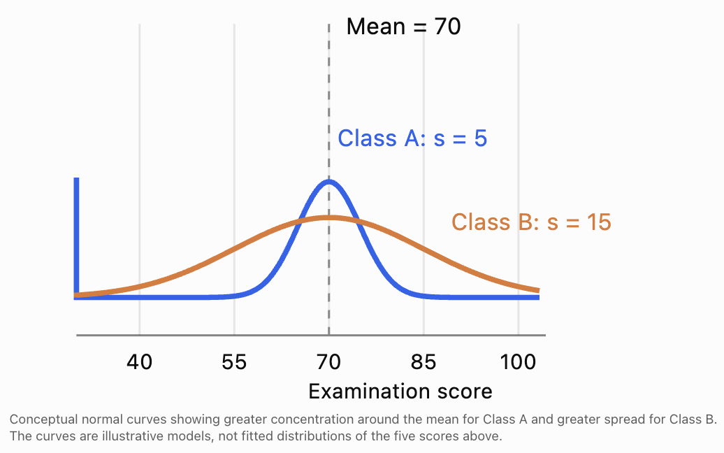
Important: A higher mean does not necessarily indicate a more desirable population. The amount of variation may be equally important.
Interpreting Differences Between Populations
When comparing populations, we should examine several characteristics.
Difference in Location
Does one population tend to have larger values than the other?
We can compare means or medians to investigate this question.
Difference in Spread
Does one population show more variability?
We can compare standard deviations, ranges, or interquartile ranges.
Difference in Shape
Are the distributions symmetric or skewed?
Does one contain more extreme observations?
Are there several clusters or peaks?
Overlap Between Distributions
Two populations may have different means but still overlap substantially.
For example:
Population A: Mean = 65, SD = 10
Population B: Mean = 70, SD = 10
Although Population B has a higher mean, many individuals in Population A may score higher than individuals in Population B.
A difference between population averages does not imply that every individual in one population has a higher value than every individual in the other.
Using Graphs to Compare Populations
Graphs help us identify differences that may be difficult to recognize from numerical summaries alone.
Side-by-Side Box Plots
Box plots show the median, quartiles, and spread of datasets.
Comparing examination scores using box plots
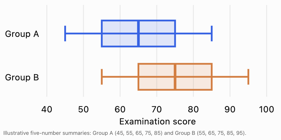
The box plots indicate that Group B generally has higher scores, but both groups have the same IQR:
IQR = 75 − 55 = 20 for Group A
IQR = 85 − 65 = 20 for Group B
The distributions also overlap.
Histograms
Histograms are useful for comparing distribution shapes, including skewness, clustering, and possible outliers.
When comparing histograms, use consistent bin widths and, where possible, the same horizontal scale.
If sample sizes differ, relative frequencies or densities may be more informative than raw frequencies.
Dot Plots
Dot plots are particularly useful for small datasets because they display individual observations.
Choosing a Graph
|
Graph |
Best use |
|---|---|
|
Side-by-side box plots |
Compare medians, quartiles and spread |
|
Histograms |
Compare distribution shapes |
|
Dot plots |
Compare small datasets |
|
Bar charts |
Compare categorical frequencies or proportions |
|
Confidence interval plots |
Compare estimates and their uncertainty |
Comparing Population Means Using Statistical Inference
Descriptive statistics show what happened in our samples.
Inferential statistics help us decide what the sample results suggest about the populations.
One common method is the two-sample t-test.
The Two-Sample t-Test
A two-sample t-test examines whether there is statistical evidence that two population means differ.
Suppose we want to compare the average mathematics scores of students using two teaching methods.
We begin with two hypotheses.
Null hypothesis (H₀):
μ₁ = μ₂
The population means are equal.
Alternative hypothesis (H₁):
μ₁ ≠ μ₂
The population means are different.
The null hypothesis represents the condition against which we test the evidence.
Worked Example: Comparing Teaching Methods
Suppose two independent random samples produce these results:
|
Statistic |
Method A |
Method B |
|---|---|---|
|
Sample size |
40 |
40 |
|
Mean score |
72 |
78 |
|
Standard deviation |
10 |
12 |
We want to determine whether the difference between the population means is statistically significant.
Step 1: Calculate the observed difference
Difference = 78 − 72 = 6
Step 2: Calculate the standard error
For independent samples, Welch's two-sample t-test uses:
SE = √(s₁²/n₁ + s₂²/n₂)
Substitute:
SE = √(10²/40 + 12²/40)
SE = √(2.5 + 3.6)
SE = √6.1
SE ≈ 2.47
Step 3: Calculate the test statistic
t = (x̄₂ − x̄₁) / SE
t = 6 / 2.47
t ≈ 2.43
Step 4: Interpret the result
Using the Welch–Satterthwaite approximation, the degrees of freedom are approximately 75.5.
The two-sided p-value is approximately 0.018.
At the 5% significance level:
p ≈ 0.018 < 0.05
Therefore, we reject the null hypothesis.
There is statistically significant evidence that the population mean examination scores differ.
The sample results suggest Method B is associated with higher scores.
However, this does not establish that Method B caused the improvement. A causal conclusion would require an appropriate experimental design, such as random assignment to teaching methods.
Understanding Statistical Significance
Statistical significance describes whether a result is sufficiently inconsistent with the null hypothesis under a chosen statistical test.
A common significance level is:
α = 0.05
The decision rule is:
-
If p ≤ 0.05, reject H₀.
-
If p > 0.05, do not reject H₀.
A p-value is the probability, assuming the null hypothesis and the statistical model are true, of obtaining a test statistic at least as extreme as the one observed.
It is not the probability that the null hypothesis is true.
Statistical Significance Versus Practical Significance
A statistically significant result is not necessarily important in practical terms.
For example, a large study may find that one teaching method increases the average examination score by only 0.3 marks.
This difference could be statistically significant because the sample size is very large.
However, an improvement of 0.3 marks might have little educational importance.
Conversely, a small study might identify a potentially important difference but lack sufficient statistical power to establish significance.
Therefore, we should consider:
-
The size of the difference.
-
The uncertainty in the estimate.
-
The sample size.
-
The practical consequences.
-
The quality of the study design.
Comparing Populations Using Confidence Intervals
A confidence interval provides a range of plausible values for a population parameter, based on the data and statistical model.
When comparing populations, we can construct a confidence interval for the difference between population means.
For independent samples, an approximate confidence interval is:
(x̄₂ − x̄₁) ± t* × SE
Here:
-
x̄₂ − x̄₁ is the observed difference.
-
t* is the appropriate critical value.
-
SE is the standard error of the difference.
Worked Example
Using our previous teaching-method data:
Observed difference = 6
SE ≈ 2.47
For a 95% confidence interval with approximately 75.5 degrees of freedom:
t* ≈ 1.99
Margin of error:
ME = 1.99 × 2.47
ME ≈ 4.91
Confidence interval:
6 ± 4.91
Lower limit:
6 − 4.91 = 1.09
Upper limit:
6 + 4.91 = 10.91
Therefore, the approximate 95% confidence interval is:
(1.09, 10.91) marks
Interpretation
We are 95% confident that the population mean score for Method B is between approximately 1.09 and 10.91 marks higher than that for Method A, under the assumptions of the analysis.
Because the interval does not contain zero, it supports the conclusion that the population means differ at the 5% significance level in a corresponding two-sided test.
A 95% confidence level means that the method used to construct the interval would capture the true population difference in approximately 95% of repeated samples under the model assumptions.
It does not mean that 95% of individual students have scores within this interval.
Understanding Effect Size
Statistical significance indicates whether there is evidence of a difference.
Effect size describes how large that difference is.
One commonly used measure for numerical data is Cohen's d.
For two independent groups:
d = (x̄₂ − x̄₁) / sₚ
where sₚ is the pooled standard deviation.
For equal sample sizes:
sₚ = √[(s₁² + s₂²)/2]
Worked Example
Using the teaching-method data:
sₚ = √[(10² + 12²)/2]
sₚ = √122
sₚ ≈ 11.05
Cohen's d:
d = 6 / 11.05
d ≈ 0.54
This indicates that the difference between the sample means is approximately 0.54 pooled standard deviations.
A commonly used, approximate interpretation is:
|
Cohen's d |
Conventional description |
|---|---|
|
0.2 |
Small |
|
0.5 |
Medium |
|
0.8 |
Large |
These are guidelines rather than universal rules. The importance of an effect depends on its context.
In this example, the observed effect is approximately medium according to these conventional benchmarks.
Comparing Population Proportions
Not every comparison involves numerical averages.
Sometimes we want to compare proportions.
For example, suppose two schools use different revision programs.
School A:
80 students passed out of 100.
School B:
90 students passed out of 100.
Step 1: Calculate Sample Proportions
School A:
p̂₁ = 80/100 = 0.80
School B:
p̂₂ = 90/100 = 0.90
Step 2: Calculate the Difference
p̂₂ − p̂₁ = 0.90 − 0.80
Difference = 0.10
School B has a pass rate 10 percentage points higher.
Step 3: Calculate the Standard Error
For an estimated difference in proportions:
SE = √[p̂₁(1 − p̂₁)/n₁ + p̂₂(1 − p̂₂)/n₂]
SE = √[(0.80 × 0.20)/100 + (0.90 × 0.10)/100]
SE = √(0.0016 + 0.0009)
SE = 0.05
Step 4: Calculate an Approximate 95% Confidence Interval
Difference ± 1.96 × SE
0.10 ± 1.96 × 0.05
0.10 ± 0.098
Confidence interval:
(0.002, 0.198)
This approximate unpooled Wald interval suggests that School B's population pass rate could be between 0.2 and 19.8 percentage points higher than School A's.
However, the lower endpoint is very close to zero, and the Wald method can be inaccurate in some situations. A score-based confidence interval is often preferable for formal analysis.
When testing equality of proportions, a pooled standard error is commonly used instead.
Paired Versus Independent Comparisons
An important decision is whether the observations in two datasets are independent or paired.
Independent Samples
Independent samples contain observations from separate, unrelated individuals or units.
Examples:
-
Comparing students from two different schools.
-
Comparing patients randomly assigned to different treatments.
-
Comparing products from two independent factories.
Common methods include:
-
Independent-samples t-test.
-
Welch's t-test.
-
Mann–Whitney U test, for appropriate distributional comparisons.
-
Two-proportion z-test.
Paired Samples
Paired samples contain related observations.
Examples:
-
Students' scores before and after a revision course.
-
Blood pressure measurements from the same patients before and after treatment.
-
Measurements from matched pairs of participants.
For paired samples, we first calculate the difference within each pair.
Difference = After − Before
Then we analyse those differences.
Worked Example: Before-and-After Scores
Five students complete a mathematics revision program.
|
Student |
Before |
After |
Difference |
|---|---|---|---|
|
A |
60 |
68 |
+8 |
|
B |
65 |
70 |
+5 |
|
C |
70 |
78 |
+8 |
|
D |
72 |
80 |
+8 |
|
E |
75 |
81 |
+6 |
Mean difference:
d̄ = (8 + 5 + 8 + 8 + 6) / 5
d̄ = 7
The students improved by an average of 7 marks.
A paired t-test could investigate whether there is evidence of a nonzero population mean improvement, provided its assumptions are appropriate.
Using the differences:
5, 6, 8, 8, 8
Sample standard deviation:
s_d = √[Σ(d − 7)² / 4]
s_d = √(8/4)
s_d ≈ 1.41
Standard error:
SE = 1.41 / √5 ≈ 0.632
Test statistic:
t = 7 / 0.632 ≈ 11.07
Degrees of freedom = 4
This provides strong evidence of a positive mean change under the paired t-test assumptions.
However, a small sample of five students limits generalization, and without a control group we cannot conclude that the revision program alone caused the improvement.
Evaluating the Quality of Statistical Evidence
Statistical calculations are only one part of comparing populations.
We must also evaluate whether the evidence is reliable.
Sample Size
Larger samples generally produce more precise estimates, assuming appropriate sampling methods.
Small samples often have greater uncertainty and are more sensitive to unusual observations.
Representative Sampling
A sample should reflect the population being studied.
For example, comparing only the highest-achieving students in one school with randomly selected students in another would produce a biased comparison.
Random sampling can reduce selection bias, although it does not eliminate every source of bias.
Confounding Variables
A confounding variable is a factor related to both the group or exposure being studied and the outcome, potentially distorting their relationship.
For example, differences in examination scores might be associated with:
-
Previous academic achievement.
-
Access to tutoring.
-
Student attendance.
-
Socioeconomic conditions.
-
Study time.
A comparison that ignores important confounding variables may lead to misleading conclusions.
Assumptions of Statistical Tests
Statistical methods depend on assumptions.
For example, a two-sample t-test generally requires:
-
Independent observations within and between groups.
-
Numerical outcomes.
-
Approximately normal sampling distributions of the means, often supported by sufficiently large samples or suitable underlying distributions.
-
No extreme data problems that invalidate the procedure.
Welch's t-test does not require equal population variances.
A paired t-test instead requires independent pairs and a suitable distribution of the within-pair differences.
Outliers
Outliers can substantially affect means and standard deviations.
When outliers are present, consider whether robust methods or comparisons of medians and distributions are more appropriate.
Multiple Comparisons
If researchers perform many statistical tests, the chance of obtaining at least one statistically significant result by chance increases.
Approaches such as Bonferroni correction or false discovery rate control can help address this problem.
Choosing an Appropriate Comparative Statistical Method
Different research questions require different statistical approaches.
|
Research situation |
Possible method |
|---|---|
|
Compare two independent means |
Welch's t-test |
|
Compare means before and after treatment |
Paired t-test |
|
Compare two independent proportions |
Two-proportion z-test |
|
Compare categorical distributions |
Chi-square test |
|
Compare independent ordinal data or distributions |
Mann–Whitney U test |
|
Compare more than two means |
ANOVA |
|
Compare groups while adjusting for other variables |
Regression or ANCOVA |
The correct method depends on the research question, measurement scale, sampling design, assumptions, and type of comparison.
For example, the Mann–Whitney U test is often described as a test of medians, but that interpretation requires additional distributional assumptions. More generally, it compares relative ranks or stochastic ordering.
Communicating Statistical Findings
A good statistical report should explain both the calculations and their meaning.
A Clear Reporting Structure
When comparing populations, include:
-
Research question: What populations or groups are being compared?
-
Descriptive statistics: What are the sample sizes, means, medians, proportions, and measures of spread?
-
Statistical method: Which test or estimation procedure was used, and why?
-
Results: What were the estimated difference, confidence interval, test statistic, and p-value where appropriate?
-
Interpretation: What do the findings suggest in the context of the investigation?
-
Limitations: What factors could affect the reliability or generalizability of the conclusions?
Example Statistical Report
A comparison of examination scores was conducted using two independent samples of 40 students. Students taught using Method A had a mean score of 72 (SD = 10), while those taught using Method B had a mean score of 78 (SD = 12). A Welch two-sample t-test found a statistically significant difference between the group means, t ≈ 2.43, p ≈ 0.018. The estimated mean difference was 6 marks, with an approximate 95% confidence interval of 1.09 to 10.91 marks. These results suggest that Method B is associated with higher examination scores. However, further information about the sampling and allocation procedures is required before drawing causal conclusions.
Notice that this report does not simply state that Method B is better.
It provides numerical evidence, identifies the statistical method, interprets the results, and acknowledges limitations.
Real-World Applications
Medicine: Comparing Treatments
Researchers may compare blood pressure reductions in patients receiving two different treatments.
They can examine mean reductions, variability, confidence intervals, and possible adverse effects.
A statistically significant difference may not necessarily be clinically meaningful.
Education: Evaluating Teaching Strategies
Schools may compare examination results, attendance rates, or student progress under different teaching approaches.
Researchers must consider previous achievement, class composition, and other potential confounders.
Manufacturing: Comparing Product Quality
Two factories may produce components with the same average dimensions but different standard deviations.
The factory with lower variation may produce more consistently sized components.
Environmental Science: Comparing Pollution Levels
Scientists may compare average particulate pollution concentrations between two cities.
However, seasonal differences, weather, measurement methods, and monitoring locations can affect the comparison.
Business: Comparing Conversion Rates
An online business might compare the proportion of visitors who register for an account under two different website designs.
For example:
Design A: 120 registrations from 2,000 visitors = 6%
Design B: 165 registrations from 2,000 visitors = 8.25%
Observed difference:
8.25% − 6% = 2.25 percentage points
Relative increase:
(8.25 − 6) / 6 × 100% = 37.5%
This is a 37.5% relative increase in the observed registration rate, not an increase of 37.5 percentage points.
A properly randomized A/B test can help determine whether the design change caused an improvement.
Common Mistakes
Mistake 1: Comparing means without considering variation
Two groups can have different means but substantial overlap.
Always examine standard deviations, distributions, and uncertainty.
Mistake 2: Assuming statistical significance means practical importance
A very small difference may be statistically significant with a sufficiently large sample.
Consider effect size and context.
Mistake 3: Interpreting a nonsignificant result as proof of equality
Failing to reject the null hypothesis does not establish that two populations are identical.
The data may be insufficiently precise to detect an important difference.
Mistake 4: Using an independent-samples test for paired data
Before-and-after measurements from the same individuals are related.
A paired analysis is generally more appropriate.
Mistake 5: Ignoring sample bias
A large biased sample may produce a precise estimate of the wrong quantity.
Sampling quality is essential.
Mistake 6: Confusing percentage points and percentage changes
An increase from 20% to 30% is:
-
10 percentage points.
-
A 50% relative increase.
These are different descriptions.
Mistake 7: Claiming causation from observational comparisons
A statistically significant association does not necessarily mean that one variable caused another.
Confounding variables and study design must be considered.
Mistake 8: Misinterpreting confidence intervals
A 95% confidence interval does not mean there is a 95% probability that the fixed population parameter lies in the calculated interval.
The 95% refers to the long-run coverage of the interval-building procedure.
Key Terms
-
Population: The complete group of individuals or observations of interest.
-
Sample: A subset of a population used for statistical analysis.
-
Population parameter: A numerical characteristic of a population.
-
Sample statistic: A numerical characteristic calculated from a sample.
-
Mean: The arithmetic average of a dataset.
-
Median: The middle value of an ordered dataset.
-
Mode: The most frequently occurring value.
-
Range: The difference between the maximum and minimum values.
-
Interquartile range (IQR): The difference between the third and first quartiles.
-
Standard deviation: A measure of variability around the mean.
-
Sampling variability: Variation in sample statistics across different random samples.
-
Standard error: The estimated standard deviation of a statistic's sampling distribution.
-
Null hypothesis: A statistical claim used as the reference point for a hypothesis test.
-
Alternative hypothesis: A competing statistical claim.
-
p-value: The probability, under the null hypothesis and model, of obtaining a test statistic at least as extreme as the observed value.
-
Significance level: A chosen threshold for deciding whether to reject the null hypothesis.
-
Confidence interval: An interval estimate constructed using a method with a specified long-run coverage rate.
-
Effect size: A measure of the magnitude of a statistical relationship or difference.
-
Independent samples: Samples consisting of unrelated observations.
-
Paired samples: Samples containing matched or repeated observations.
-
Confounding variable: A variable that can distort the relationship between an exposure and an outcome.
-
Statistical significance: Evidence against a null hypothesis according to a specified statistical test and significance level.
-
Practical significance: The real-world importance of an observed effect.
Key Takeaways
-
Comparing populations involves examining differences in central tendency, spread, shape, and other statistical characteristics.
-
Sample statistics provide estimates of unknown population parameters.
-
Means and medians describe typical values, while standard deviations and IQRs describe variation.
-
Graphs such as box plots, histograms, and dot plots help reveal patterns and differences.
-
Statistical tests assess how strongly the data contradict a specified null hypothesis.
-
Confidence intervals provide information about both the estimated difference and its uncertainty.
-
Effect sizes help describe the magnitude of differences.
-
Independent and paired data require different analytical approaches.
-
Sample size, bias, confounding variables, and statistical assumptions affect the reliability of conclusions.
-
Clear statistical communication includes numerical evidence, contextual interpretation, and appropriate limitations.
Check Your Understanding
Question 1: Comparing Means
Two groups of students receive the following examination scores.
Group A: 60, 70, 75, 80, 85
Group B: 65, 75, 80, 85, 95
Calculate the mean for each group and determine which group has the higher mean.
Answer
Group A:
Mean = (60 + 70 + 75 + 80 + 85) / 5
Mean = 370 / 5 = 74
Group B:
Mean = (65 + 75 + 80 + 85 + 95) / 5
Mean = 400 / 5 = 80
Difference:
80 − 74 = 6
Group B has a mean score 6 marks higher than Group A.
This describes the observed samples but does not by itself establish a population difference.
Question 2: Comparing Variation
Two datasets have the following characteristics:
Dataset A: Mean = 50, SD = 4
Dataset B: Mean = 50, SD = 12
Which dataset has greater variation?
Answer
Dataset B has greater variation because its standard deviation is larger.
The values in Dataset B tend to be more widely dispersed around the mean.
Both datasets have the same mean, but their consistency differs.
Question 3: Interpreting Statistical Significance
A statistical test comparing two population means produces:
p = 0.032
The significance level is:
α = 0.05
What conclusion should be reached?
Answer
Since:
0.032 < 0.05
We reject the null hypothesis.
There is statistically significant evidence of a difference between the population means, assuming the test and its assumptions are appropriate.
This does not necessarily mean that the difference is large or practically important.
Question 4: Confidence Intervals
A study estimates that the mean difference between two populations is 8 units.
The standard error is 3 units.
Calculate an approximate 95% confidence interval using a critical value of 1.96.
Answer
Confidence interval:
Difference ± 1.96 × SE
= 8 ± 1.96 × 3
= 8 ± 5.88
Lower limit:
8 − 5.88 = 2.12
Upper limit:
8 + 5.88 = 13.88
95% confidence interval: (2.12, 13.88)
Because the interval does not include zero, it suggests a positive population mean difference under the normal approximation.
Question 5: Comparing Proportions
School A has 120 students who pass an examination out of 150 students.
School B has 135 students who pass out of 150.
Calculate the pass rates and their difference.
Answer
School A:
120 / 150 × 100% = 80%
School B:
135 / 150 × 100% = 90%
Difference:
90% − 80% = 10 percentage points
School B's observed pass rate is 10 percentage points higher.
Relative increase:
(90 − 80) / 80 × 100% = 12.5%
Therefore, School B's pass rate is 12.5% higher relative to School A's rate.
Question 6: Choosing a Statistical Method
A researcher measures the reaction times of 30 participants before and after drinking coffee.
Should the researcher use an independent-samples t-test or a paired t-test?
Answer
A paired t-test is appropriate because the same participants are measured twice.
The researcher should calculate each participant's change in reaction time and analyse the differences.
This accounts for the relationship between the two measurements.
Question 7: Evaluating Statistical Evidence
A study reports that a new teaching method improves examination scores by an average of 2 marks.
The difference is statistically significant, with p = 0.001.
Does this prove that the teaching method is educationally important?
Answer
No.
The p-value provides evidence against the null hypothesis but does not describe the educational importance of the difference.
A 2-mark improvement may or may not be meaningful, depending on the examination scale, consequences, costs, and other factors.
We should also examine the confidence interval, effect size, study design, and possible confounding variables.
Question 8: Comparing Two Populations
Two independent samples have the following characteristics:
Population A sample:
n₁ = 50, x̄₁ = 100, s₁ = 15
Population B sample:
n₂ = 50, x̄₂ = 108, s₂ = 20
Calculate the standard error of the difference and the Welch t-statistic.
Answer
Step 1: Calculate the standard error.
SE = √(s₁²/n₁ + s₂²/n₂)
SE = √(15²/50 + 20²/50)
SE = √(225/50 + 400/50)
SE = √(4.5 + 8)
SE = √12.5
SE ≈ 3.54
Step 2: Calculate the difference.
Difference = 108 − 100 = 8
Step 3: Calculate the t-statistic.
t = 8 / 3.54
t ≈ 2.26
This statistic can be used with the appropriate Welch degrees of freedom to calculate a p-value.
The result suggests that Population B may have a higher mean, but a complete inferential conclusion requires the test assumptions, degrees of freedom, and chosen significance level.
Question 9: Identifying Bias
A researcher compares the examination scores of students attending two schools.
For School A, the researcher selects only students enrolled in advanced mathematics classes.
For School B, the researcher selects students randomly from all mathematics classes.
Explain why the comparison may be misleading.
Answer
The samples were selected using different procedures.
School A's sample includes only advanced mathematics students, who may have higher achievement than the overall student population.
School B's sample represents a wider range of students.
Therefore, the observed difference may reflect selection bias rather than a genuine difference between the schools.
A better approach would be to use comparable sampling methods and account for relevant student characteristics.
Question 10: Communicating a Statistical Conclusion
A researcher compares the average daily exercise time of two groups.
Group A:
Mean = 35 minutes
Group B:
Mean = 42 minutes
The estimated difference is 7 minutes, with a 95% confidence interval from 2 to 12 minutes.
Write an appropriate statistical conclusion.
Answer
Group B exercised for an average of 7 minutes longer per day than Group A in the samples studied.
The 95% confidence interval suggests that the population mean difference is plausibly between 2 and 12 minutes, under the statistical model.
Because the confidence interval does not include zero, the results provide evidence of a difference between the population means.
However, the practical importance of this difference depends on the research context, and the reliability of the conclusion depends on the study design, sampling methods, and statistical assumptions.
Final Reflection
Comparing populations is one of the most important applications of statistics because it allows us to move beyond individual observations and investigate broader patterns.
A strong statistical comparison does not simply ask, "Which group has the higher average?"
It also asks:
-
How large is the difference?
-
How much variation exists within each group?
-
How reliable is the evidence?
-
Could the difference be explained by sampling variability or bias?
-
Is the difference meaningful in the real world?
-
What conclusions can we reasonably communicate?
By combining descriptive statistics, graphical analysis, statistical inference, and careful interpretation, we can make informed comparisons and communicate findings accurately and responsibly.
5. Interpreting Statistical Studies
Learning outcomes
- I can critically evaluate statistical investigations.
- I can identify misleading conclusions.
- I can distinguish correlation from causation.
- I can recognise limitations of statistical studies.
- I can evaluate evidence using statistics.
Introduction
Every day, we encounter claims based on statistics. News articles report that certain foods improve health, advertisements claim that products are more effective than their competitors, and researchers publish studies suggesting relationships between different factors.
Consider the following headlines:
-
"Students who eat breakfast achieve higher examination scores."
-
"People who exercise regularly live longer."
-
"A new teaching method improves mathematics performance by 25%."
-
"Using social media causes students to perform poorly at school."
-
"A survey shows that 90% of people prefer our product."
These statements may sound convincing, especially when they include numbers, percentages, or references to scientific research.
But how can we determine whether the conclusions are justified?
For example, if students who eat breakfast tend to achieve higher examination scores, does this prove that eating breakfast causes better academic performance? Could other factors, such as sleep, family circumstances, or study habits, explain the relationship?
Interpreting statistical studies means examining how data were collected, how they were analysed, and whether the conclusions are supported by reliable evidence.
A statistically literate person does not simply accept a conclusion because it contains numbers. Instead, they ask critical questions about sampling, bias, study design, correlation, causation, uncertainty, and the limitations of the investigation.
These skills are essential for making informed decisions in science, medicine, education, economics, business, and everyday life.
Understanding Statistical Investigations
A statistical investigation is a systematic process used to collect, analyse, interpret, and communicate data in order to answer a research question.
A well-designed investigation typically follows several stages.
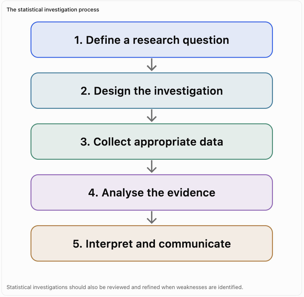
Stage 1: Define the Research Question
A research question should be specific and measurable.
Weak question:
"Does technology help students?"
Improved question:
"Do Grade 9 students who use an online revision program for four weeks achieve higher average test scores than students using printed revision materials?"
The improved question identifies the population, comparison, outcome, and time period.
Stage 2: Design the Investigation
Researchers decide:
-
Who will participate?
-
How will participants be selected?
-
What variables will be measured?
-
Will the study be observational or experimental?
-
How will bias and confounding variables be addressed?
-
What statistical methods will be used?
Stage 3: Collect Data
Researchers gather information using methods such as surveys, experiments, observations, or existing records.
Data collection should be accurate, consistent, ethical, and appropriate for the research question.
Stage 4: Analyse the Data
Researchers may calculate means, proportions, standard deviations, correlations, confidence intervals, or statistical test results.
Graphs can help identify patterns and unusual observations.
Stage 5: Interpret and Communicate Findings
Researchers explain what the results suggest, assess uncertainty, and identify limitations.
A strong conclusion distinguishes what the evidence actually establishes from what remains uncertain.
Evaluating the Quality of a Statistical Study
Not all statistical investigations provide equally reliable evidence.
Before accepting a conclusion, we should examine the quality of the study.
The Research Question
A good investigation begins with a clear research question.
For example:
"Are students happier when using technology?"
This is vague because happiness and technology use have not been clearly defined.
A more precise question is:
"Is daily recreational screen time associated with self-reported wellbeing scores among students aged 13–16?"
This identifies measurable variables and a defined population.
The Population and Sample
The population is the entire group that researchers want to investigate.
The sample is the subset from which data are collected.
Suppose a researcher wants to investigate the study habits of all secondary school students in Singapore.
If the researcher surveys only students from one advanced mathematics class, the sample may not represent the intended population.
This creates a risk of selection bias.
Sample Size
Larger samples generally provide more precise estimates, provided that the sampling method is appropriate.
However, a large sample does not automatically guarantee reliable conclusions.
A survey of 10,000 people selected using a biased method may be less representative than a carefully selected random sample of 500 people.
Measurement Quality
Researchers must ensure that variables are measured consistently and accurately.
For example, asking students to estimate how many hours they studied last month may produce inaccurate responses because students may not remember their study time.
Using a daily study log might produce more reliable measurements, although self-reporting can still introduce errors.
Recognising Bias in Statistical Studies
Bias is a systematic error that causes a statistical estimate or conclusion to deviate from the quantity it is intended to represent.
Bias can occur during sampling, measurement, analysis, or reporting.
Selection Bias
Selection bias occurs when the process of selecting participants produces a sample that differs systematically from the target population.
Example
A school surveys only students attending an optional after-school mathematics club to determine whether all students enjoy mathematics.
Students attending the club may be more interested in mathematics than the average student.
The results may therefore overestimate enjoyment.
Voluntary Response Bias
Voluntary response bias occurs when people choose whether to participate and those who respond differ systematically from those who do not.
Example
A website asks visitors to complete an optional survey about customer satisfaction.
People with very positive or very negative experiences may be more likely to respond.
The results may not represent all customers.
Nonresponse Bias
Nonresponse bias occurs when selected participants do not respond and their characteristics differ from those who participate.
Example
A survey about working hours receives responses mainly from employees who have flexible schedules.
Employees working longer or irregular hours may be underrepresented.
Response Bias
Response bias occurs when answers are systematically influenced by factors such as question wording, social expectations, or inaccurate recall.
Consider two questions:
"Do you agree that responsible students should complete homework every day?"
"How many days per week do you believe students should complete homework?"
The first question contains leading language that may influence responses.
The second is more neutral.
Confirmation Bias
Confirmation bias occurs when researchers or readers give greater attention to evidence supporting their existing beliefs.
For example, someone who believes that online learning is ineffective might focus on studies reporting poor results while ignoring studies showing benefits.
Publication Bias
Publication bias occurs when studies with statistically significant or striking findings are more likely to be published or promoted than studies with inconclusive findings.
This can distort the overall impression of the available evidence.
Correlation and Causation
One of the most important skills in interpreting statistical studies is distinguishing between correlation and causation.
What Is Correlation?
Correlation describes a statistical relationship between two variables.
When two variables are correlated, their values tend to vary together in a systematic way.
Correlation may be positive, negative, or approximately zero.
Positive Correlation
A positive correlation occurs when larger values of one variable tend to be associated with larger values of another.
Examples include:
-
Height and mass among growing children.
-
Hours studied and examination performance.
-
Outdoor temperature and ice cream sales.
Negative Correlation
A negative correlation occurs when larger values of one variable tend to be associated with smaller values of another.
Examples include:
-
Distance travelled and fuel remaining in a vehicle.
-
Price and quantity demanded under some market conditions.
-
Time spent practising a skill and the number of errors made.
No Linear Correlation
When there is no linear correlation, the variables do not display a clear straight-line relationship.
However, they may still have a nonlinear relationship.
Three possible correlation patterns
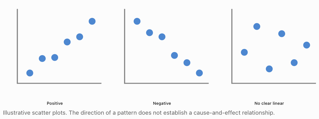
The Correlation Coefficient
The Pearson correlation coefficient, represented by r, measures the direction and strength of a linear relationship.
Its value lies between −1 and +1.
|
Value of r |
Interpretation |
|---|---|
|
+1 |
Perfect positive linear correlation |
|
+0.8 |
Strong positive linear correlation |
|
+0.3 |
Weak positive linear correlation |
|
0 |
No linear correlation |
|
−0.3 |
Weak negative linear correlation |
|
−0.8 |
Strong negative linear correlation |
|
−1 |
Perfect negative linear correlation |
These descriptions are approximate and depend on the research context.
The coefficient can be calculated using:
r = Σ[(x − x̄)(y − ȳ)] / √[Σ(x − x̄)² × Σ(y − ȳ)²]
For example, if a study finds:
r = 0.85
between study hours and examination scores, this indicates a strong positive linear relationship in the observed data.
It does not prove that increasing study hours causes higher scores.
What Is Causation?
Causation occurs when a change in one factor produces a change in another.
For example, in a controlled physical experiment, increasing the applied net force on an object of constant mass causes greater acceleration, according to Newton's Second Law.
In statistical investigations involving human behaviour, identifying causation is often more difficult because many variables may influence the outcome.
Why Correlation Does Not Prove Causation
Consider this example:
A study finds that ice cream sales and drowning incidents both increase during summer.
Does buying ice cream cause drowning?
No.
A third variable, hot weather, can influence both.
A confounding variable can create an association
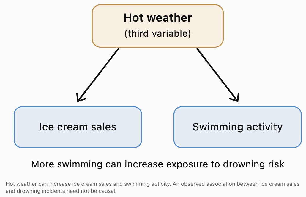
Other Explanations for Correlation
Reverse causation
Researchers may incorrectly assume the direction of cause and effect.
For example, a study might find that students receiving extra tutoring have lower examination scores.
It would be misleading to conclude that tutoring causes poor performance.
Students who are already struggling may be more likely to receive tutoring.
Coincidence
Two variables may appear correlated simply by chance, especially when many possible relationships are examined.
Confounding variables
Other factors may influence both variables and create or distort the observed relationship.
Selection effects
The way participants are selected can create an apparent relationship that does not exist in the wider population.
Observational Studies and Experiments
The type of investigation strongly affects the conclusions researchers can draw.
Observational Studies
In an observational study, researchers measure variables without assigning participants to treatments or deliberately manipulating the exposure of interest.
For example, researchers might compare examination results among students who independently choose different revision methods.
Observational studies can identify associations and provide valuable evidence.
However, differences between groups may be caused by confounding variables.
Controlled Experiments
In a controlled experiment, researchers deliberately assign treatments or conditions and measure the resulting outcomes.
A randomized controlled experiment is particularly useful for investigating causation.
For example, researchers might randomly assign students to:
-
Group A: Traditional revision materials.
-
Group B: Interactive revision materials.
Both groups complete the same assessment after four weeks.
Random assignment helps balance both known and unknown confounding variables across groups, especially in sufficiently large studies.
Random Sampling Versus Random Assignment
These concepts serve different purposes.
|
Random sampling |
Random assignment |
|---|---|
|
Selects participants from a population |
Allocates participants to experimental groups |
|
Helps improve population representativeness |
Helps reduce confounding between treatment groups |
|
Supports generalization |
Supports causal inference |
|
Does not automatically establish causation |
Does not automatically ensure population representativeness |
An experiment can have strong internal validity but limited generalizability if its participants are not representative of the wider population.
Identifying Misleading Statistical Conclusions
Statistical claims can be misleading even when the underlying numbers are mathematically correct.
Misleading Percentages
Suppose an advertisement states:
"Our program increased student success by 100%!"
This sounds impressive.
However, imagine the pass rate increased from 2% to 4%.
Relative increase:
(4 − 2) / 2 × 100% = 100%
Absolute increase:
4% − 2% = 2 percentage points
The statement is mathematically correct but omits important context.
Always ask whether a reported percentage is an absolute change or a relative change.
Misleading Graph Scales
A graph with a truncated vertical axis can make a small difference appear dramatic.
Cherry-Picking Data
Cherry-picking occurs when someone selects only data that support a desired conclusion.
For example, a company might report sales growth during its best three months while ignoring the rest of the year.
A fair analysis should consider the relevant full dataset and explain any exclusions.
Small or Unrepresentative Samples
Suppose a company claims:
"Nine out of ten customers recommend our product."
If only ten customers were surveyed, the estimate is highly uncertain.
If those customers were selected from a group of enthusiastic supporters, the result may also be biased.
Confusing Statistical Significance With Importance
A study may report a statistically significant improvement of 0.2 marks on a 100-mark examination.
This result could be statistically detectable but educationally unimportant.
We must consider the magnitude and consequences of the effect.
Evaluating Evidence Using Descriptive Statistics
Descriptive statistics help summarize the observations in a study.
However, different statistics reveal different aspects of the data.
Worked Example: Comparing Two Teaching Programs
Suppose researchers collect the following results:
|
Statistic |
Program A |
Program B |
|---|---|---|
|
Students |
50 |
50 |
|
Mean score |
72 |
78 |
|
Median score |
74 |
79 |
|
Standard deviation |
8 |
15 |
Step 1: Compare the means
78 − 72 = 6
Program B has a sample mean 6 marks higher.
Step 2: Compare the medians
79 − 74 = 5
Program B also has a higher median.
Step 3: Compare variation
Program A: SD = 8
Program B: SD = 15
Program B has substantially greater variability.
Step 4: Interpret the findings
Program B has higher typical scores in this sample, but its results are less consistent.
Some students may perform very well under Program B, while others may perform poorly.
Step 5: Evaluate limitations
Before concluding that Program B is more effective, we should ask whether students were randomly assigned, whether the assessments were comparable, and whether other differences between groups could explain the results.
Evaluating Evidence Using Confidence Intervals
A confidence interval provides an estimate of uncertainty around a population parameter.
Suppose a study estimates that a new teaching program improves scores by 5 marks.
Its 95% confidence interval for the mean improvement relative to a comparison program is:
(1, 9)
This suggests that the true mean difference is plausibly between 1 and 9 marks, assuming the statistical model is appropriate.
Because the interval does not contain zero, it provides evidence of a positive difference under a corresponding two-sided 5% test.
Now consider a second study:
Estimated difference = 5 marks
95% confidence interval:
(−3, 13)
Although both studies estimate the same difference, the second interval is much wider and includes zero.
The second study provides less precise evidence about the population difference.
Confidence Interval Width
Narrow confidence intervals generally indicate greater precision.
Wide confidence intervals indicate greater uncertainty.
Confidence interval width depends on factors including sample size, variability, confidence level, and the estimation method.
Evaluating Evidence Using Hypothesis Tests
A hypothesis test evaluates how compatible observed data are with a specified null hypothesis.
Worked Example: A New Learning Program
A study compares two teaching programs.
The null hypothesis is:
H₀: μ₁ = μ₂
The alternative hypothesis is:
H₁: μ₁ ≠ μ₂
The test produces:
p = 0.03
At a significance level of 0.05:
0.03 < 0.05
Therefore, the researchers reject the null hypothesis.
There is statistically significant evidence of a difference between the population means.
However, the p-value does not tell us:
-
How large the difference is.
-
Whether the difference is educationally important.
-
Whether the study was biased.
-
Whether one teaching method caused the difference.
-
The probability that the null hypothesis is true.
A p-value should be interpreted alongside the effect size, confidence interval, research design, and data quality.
Understanding Study Limitations
Every statistical investigation has limitations.
Recognising these limitations is essential for evaluating the strength of its conclusions.
Sampling Limitations
A sample may not represent the intended population.
For example, results from students at one school may not generalize to students across an entire country.
Measurement Limitations
Measurements may be inaccurate or inconsistent.
Self-reported exercise time, for example, may differ from actual exercise time.
Confounding Variables
Unmeasured variables may influence the results.
An observational study linking screen time to examination performance might be affected by sleep, prior achievement, or home environment.
Small Sample Sizes
Small samples often produce imprecise estimates and can be strongly affected by unusual observations.
Short Study Duration
A short investigation may not reveal long-term effects.
For example, a teaching intervention may improve short-term test scores without improving long-term retention.
Missing Data
If participants drop out or fail to provide information, the remaining data may be unrepresentative.
Lack of Replication
A single study may produce an unusual result by chance.
Replication helps determine whether findings are consistent across different samples and settings.
Generalizability
A conclusion may apply only to the population, conditions, and setting studied.
Researchers should avoid extending results beyond the evidence.
Evaluating Evidence Using Effect Size
Statistical significance tells us whether the data provide evidence against a null hypothesis.
Effect size describes the magnitude of an observed difference or relationship.
For two independent groups, a common standardized effect size is Cohen's d.
d = (x̄₂ − x̄₁) / sₚ
Here, sₚ is the pooled standard deviation.
Worked Example
Suppose:
Group A mean = 70
Group B mean = 76
Pooled standard deviation = 12
Then:
d = (76 − 70) / 12
d = 6 / 12
d = 0.5
The observed mean difference is half a pooled standard deviation.
A conventional interpretation is that this represents a medium-sized effect.
However, whether the effect is practically important depends on the situation.
For example, a modest improvement in a medical treatment could be important if it prevents serious complications, while a similar standardized difference in another context might have little practical consequence.
Evaluating Multiple Statistical Studies
When several studies investigate the same question, their findings may differ.
For example:
|
Study |
Sample size |
Estimated improvement |
95% confidence interval |
|---|---|---|---|
|
A |
40 |
+6 marks |
−2 to +14 |
|
B |
200 |
+5 marks |
+2 to +8 |
|
C |
500 |
+4 marks |
+2 to +6 |
All three studies estimate a positive improvement.
However, Study A has a wide confidence interval that includes zero, indicating substantial uncertainty.
Studies B and C provide more precise estimates, assuming the methods and data are reliable.
We should not automatically conclude that Study C is the best study simply because it has the largest sample.
Study quality, participant selection, measurement accuracy, confounding, and statistical methods must also be considered.
Systematic Reviews and Meta-Analyses
A systematic review uses a structured method to identify, evaluate, and summarize relevant studies.
A meta-analysis statistically combines results from multiple studies when appropriate.
These approaches can provide stronger evidence than a single study, but their reliability depends on the quality, comparability, and completeness of the included studies.
Combining several biased studies does not automatically eliminate bias.
Real-World Applications
Health and Medicine
Suppose a newspaper reports:
"People who drink green tea have a lower risk of heart disease."
Before accepting a causal interpretation, we should ask whether the study was observational or experimental, whether other lifestyle factors were considered, and how large and precise the estimated association was.
People who drink green tea may differ from other people in diet, exercise, income, or other characteristics.
Education
A school reports that examination scores increased after introducing a new online learning platform.
However, the increase might also reflect changes in teaching, examination difficulty, student composition, or additional revision time.
A comparison with an appropriate control group would provide stronger evidence about the platform's effect.
Advertising
A company advertises:
"95% of users experienced improvement."
Important questions include how improvement was measured, how many people participated, how participants were selected, and whether the study included a comparison group.
Environmental Science
Researchers report a correlation between air pollution and respiratory illness.
Statistical evidence can help identify an association, but causal interpretation requires careful consideration of other factors, exposure measurement, timing, and the broader body of scientific evidence.
Social Media and Technology
A study reports that students who spend more time on social media have lower average examination scores.
Possible explanations include:
-
Social media use affecting study time.
-
Students struggling academically spending more time online.
-
Other factors influencing both social media use and academic performance.
The association alone cannot establish which explanation is correct.
A Practical Framework for Critically Evaluating Statistical Claims
When reading a statistical study or news article, use the following questions.
Statistical study evaluation checklist
0 of 12 reviewed
A study that performs well on these criteria is generally more trustworthy than one that ignores important methodological weaknesses.
However, no checklist can replace careful consideration of the specific research question and study design.
Common Mistakes
Mistake 1: Assuming correlation proves causation
A relationship between two variables does not automatically mean one causes the other.
Look for confounding variables, reverse causation, and alternative explanations.
Mistake 2: Believing a large sample eliminates all bias
Large samples can reduce random sampling error, but they cannot automatically correct systematic bias.
Mistake 3: Treating a small p-value as proof that a hypothesis is true
A small p-value provides evidence against the null hypothesis under the model assumptions. It does not prove the alternative hypothesis with certainty.
Mistake 4: Ignoring absolute differences when reading percentages
A 100% relative increase may represent a change from 1% to 2%, which is only one percentage point.
Mistake 5: Assuming a statistically significant result must be important
Statistical significance and practical importance are different concepts.
Mistake 6: Ignoring the scale of a graph
A truncated or inconsistent scale can exaggerate or conceal differences.
Mistake 7: Generalizing beyond the population studied
Results from a small or narrowly selected group may not apply to a wider population.
Mistake 8: Accepting conclusions without examining study design
Observational studies, randomized experiments, and surveys support different types of conclusions.
Mistake 9: Ignoring uncertainty
A point estimate without a confidence interval or another measure of uncertainty may give an incomplete picture.
Mistake 10: Selecting only evidence that supports a preferred conclusion
Reliable statistical interpretation considers the relevant evidence as a whole, including contradictory findings and limitations.
Key Terms
-
Statistical investigation: A systematic process of collecting, analysing, and interpreting data to answer a research question.
-
Population: The complete group of individuals or observations of interest.
-
Sample: A subset of a population.
-
Representative sample: A sample that adequately reflects the relevant characteristics of its target population.
-
Bias: A systematic error that distorts a statistical estimate or conclusion.
-
Selection bias: Bias caused by the process used to select participants.
-
Response bias: Systematic distortion in participants' answers.
-
Nonresponse bias: Bias arising when nonrespondents differ from respondents in relevant ways.
-
Confirmation bias: The tendency to favour information supporting existing beliefs.
-
Publication bias: Distortion arising when certain study results are more likely to be published.
-
Correlation: A statistical relationship between variables.
-
Causation: A relationship in which a change in one factor produces a change in another.
-
Correlation coefficient: A numerical measure of the direction and strength of a relationship.
-
Confounding variable: A variable that can distort an observed relationship between an exposure and an outcome.
-
Observational study: A study in which researchers observe variables without assigning the exposure or treatment of interest.
-
Controlled experiment: An investigation in which researchers assign conditions or treatments and compare outcomes.
-
Random assignment: Allocation of participants to experimental groups using a random process.
-
Random sampling: Selection of participants from a population using a random process.
-
Null hypothesis: A statistical claim used as the reference point for a hypothesis test.
-
p-value: The probability, under the null hypothesis and statistical model, of observing a test statistic at least as extreme as the one obtained.
-
Statistical significance: Evidence against a null hypothesis according to a specified statistical test and significance level.
-
Confidence interval: An interval estimate constructed using a procedure with a specified long-run coverage rate.
-
Effect size: A measure of the magnitude of a difference or relationship.
-
Practical significance: The real-world importance of an observed result.
-
Generalizability: The extent to which findings apply beyond the individuals or conditions studied.
-
Replication: Repeating a study to assess whether findings are consistent.
-
Systematic review: A structured synthesis of research evidence.
-
Meta-analysis: A statistical method for combining results from multiple studies.
Key Takeaways
-
Statistical studies must be evaluated critically rather than accepted solely because they contain numerical evidence.
-
Reliable investigations require clear research questions, appropriate samples, accurate measurements, and suitable analytical methods.
-
Bias can arise during participant selection, data collection, analysis, and reporting.
-
Correlation describes an association between variables, while causation requires evidence that one factor influences another.
-
Randomized controlled experiments can provide stronger causal evidence than simple observational comparisons when appropriately designed.
-
Misleading statistical claims may involve selective reporting, confusing percentages, inappropriate graphs, or unsupported causal conclusions.
-
Confidence intervals, effect sizes, p-values, and descriptive statistics provide different but complementary information.
-
Statistical significance does not necessarily imply practical importance.
-
Every study has limitations that should be acknowledged when interpreting findings.
-
Strong statistical conclusions are supported by reliable evidence, appropriate methods, and clear communication of uncertainty.
Check Your Understanding
Question 1: Identifying Bias
A researcher wants to determine whether students enjoy mathematics.
The researcher surveys 100 students attending an optional mathematics enrichment club.
Explain why the results may be biased.
Answer
The sample may suffer from selection bias because students attending a mathematics enrichment club are likely to have a greater interest in mathematics than the general student population.
Therefore, the sample may overestimate how much students enjoy mathematics.
A better approach would be to select a representative sample from the wider student population.
Question 2: Correlation Versus Causation
A study finds that students who spend more time studying tend to achieve higher examination scores.
The correlation coefficient is:
r = 0.82
What does this indicate? Does it prove causation?
Answer
A correlation coefficient of 0.82 indicates a strong positive linear relationship between study time and examination scores.
Students who study more tend to achieve higher scores in the observed data.
However, correlation does not establish causation.
Other factors, such as motivation, previous academic achievement, and access to learning resources, may influence both study time and performance.
A carefully designed experiment could provide stronger evidence about the causal effect of additional study time.
Question 3: Misleading Percentages
A company reports that its product increased customer satisfaction by 50%.
The original satisfaction rate was 40%.
Calculate the new satisfaction rate if the claim refers to a relative increase.
Answer
Increase = 50% of 40%
Increase = 0.50 × 40% = 20 percentage points
New satisfaction rate:
40% + 20% = 60%
The satisfaction rate increased from 40% to 60%.
This is a relative increase of 50%, but an absolute increase of 20 percentage points.
Question 4: Interpreting a p-value
A statistical test produces:
p = 0.008
The significance level is:
α = 0.05
What conclusion should be reached?
Answer
Since:
0.008 < 0.05
We reject the null hypothesis.
The data provide statistically significant evidence against the null hypothesis under the assumptions of the test.
However, the p-value does not establish the size, practical importance, or causal nature of the effect.
Question 5: Evaluating Study Design
A school introduces a new teaching program.
At the end of the year, average examination scores increase from 70 to 78.
The school concludes that the program caused the improvement.
Explain why this conclusion may be unjustified.
Answer
The improvement could be associated with several other factors, including:
-
Changes in student ability.
-
Different examination difficulty.
-
Additional revision opportunities.
-
Changes in teaching staff.
-
Differences in attendance.
Without an appropriate comparison group or stronger experimental design, the school cannot confidently attribute the improvement to the new program.
The evidence establishes that average scores increased, but not necessarily why they increased.
Question 6: Interpreting Confidence Intervals
A study estimates that a new treatment reduces recovery time by an average of 3 days compared with an existing treatment.
The 95% confidence interval for the reduction is:
(−1, 7) days
What does this suggest?
Answer
The estimated mean reduction is 3 days, but the confidence interval includes zero.
It also includes negative values, which would indicate that the new treatment increases recovery time.
Therefore, the results do not establish a statistically significant difference at the 5% level under the corresponding two-sided test.
The evidence is compatible with a range of effects, from a small disadvantage to a substantial benefit.
More precise evidence may be needed.
Question 7: Comparing Statistical Evidence
Two studies investigate the same teaching method.
Study A:
n = 30
Estimated improvement = 5 marks
95% confidence interval = (−4, 14)
Study B:
n = 400
Estimated improvement = 5 marks
95% confidence interval = (3, 7)
Which study provides more precise evidence?
Answer
Study B provides more precise evidence because its confidence interval is narrower.
Study A interval width:
14 − (−4) = 18
Study B interval width:
7 − 3 = 4
Both studies estimate the same improvement, but Study B has substantially less uncertainty.
However, greater precision does not automatically mean lower bias. Study design and sampling quality must still be evaluated.
Question 8: Recognising a Confounding Variable
A study finds that people who own expensive sports equipment tend to exercise more frequently.
The researcher concludes that purchasing expensive equipment causes people to exercise more.
Identify a possible confounding variable.
Answer
One possible confounding variable is income.
People with higher incomes may be more likely to purchase expensive equipment and may also have greater access to fitness facilities or recreational opportunities.
Another possible factor is existing interest in fitness.
People who already exercise frequently may be more willing to purchase expensive equipment.
Therefore, the observed association does not prove that buying expensive equipment causes increased exercise.
Question 9: Evaluating Statistical Significance
A large study finds that a new educational program improves examination scores by an average of 0.4 marks out of 100.
The result is statistically significant, with:
p = 0.001
Should the school automatically adopt the program?
Answer
No.
Although the result is statistically significant, the average improvement is very small.
The school should also consider:
-
The cost of the program.
-
The time required to implement it.
-
The confidence interval around the improvement.
-
Whether the effect is consistent across different students.
-
Whether the study supports a causal conclusion.
-
Whether the improvement has meaningful educational consequences.
Statistical significance alone is insufficient for making an informed decision.
Question 10: Critical Evaluation of a Statistical Claim
A news article states:
"Scientists prove that drinking coffee makes students more intelligent."
The article describes an observational study of 200 university students.
Students who drank coffee regularly achieved an average test score of 78, while students who did not drink coffee achieved an average score of 73.
Identify at least four problems with the headline or conclusion.
Answer
Problem 1: Causation is not established.
The study is observational, so it cannot by itself prove that coffee causes higher intelligence or better performance.
Problem 2: Confounding variables may exist.
Coffee consumption may be associated with study habits, sleep, workload, age, or other factors.
Problem 3: Test scores do not directly measure intelligence.
The study measured examination performance, not necessarily intelligence.
Problem 4: Statistical uncertainty is not reported.
The article does not provide standard deviations, confidence intervals, or hypothesis test results.
Problem 5: Generalizability is uncertain.
The sample consists of 200 university students, and the sampling method is unknown.
Improved conclusion:
"In a study of 200 university students, regular coffee drinkers had an average test score 5 marks higher than non-coffee drinkers. However, the observational design does not establish that coffee consumption caused the difference."
This conclusion accurately describes the observed association without making unsupported causal claims.
Final Reflection
Statistics can reveal valuable information about the world, but numbers alone do not guarantee reliable conclusions.
A strong statistical thinker examines not only what the data show, but also how the data were obtained, what assumptions were made, how uncertainty was handled, and whether alternative explanations are possible.
When interpreting any statistical study, three questions are particularly important:
What does the evidence actually show?
What conclusions are justified by the research design and statistical analysis?
What limitations or uncertainties should be considered before accepting the findings?
Developing these habits allows us to distinguish strong evidence from misleading claims and make better-informed decisions in education, science, health, business, and everyday life.