Statistical Inference
3. Errors in Statistical Testing
Learning outcomes
- I can distinguish between Type I and Type II errors.
- I can explain statistical significance.
- I can interpret significance levels.
- I can evaluate statistical conclusions.
- I can explain limitations of hypothesis testing.
Introduction
Statistical hypothesis testing helps researchers make decisions using sample data. However, because samples contain uncertainty, statistical decisions can sometimes be wrong.
Imagine a medical screening test that indicates a person has a particular disease. The result could be correct, but it could also be a false positive. Alternatively, a screening test might fail to detect a disease that is actually present.
A similar problem occurs in statistical hypothesis testing.
A researcher may:
-
Reject a null hypothesis that is actually true.
-
Fail to reject a null hypothesis that is actually false.
These mistakes are known as Type I and Type II errors.
Understanding these errors is essential because statistical significance does not guarantee that a conclusion is correct, important, or reliable.
In this lesson, we will explore how errors occur, how significance levels influence decisions, how statistical power affects the detection of real effects, and why hypothesis tests must be interpreted carefully.
Review: The Logic of Hypothesis Testing
A hypothesis test evaluates a claim about a population parameter using sample data.
The two competing hypotheses are:
Null hypothesis (H₀): The reference claim being tested, often representing no difference or no effect.
Alternative hypothesis (H₁ or Hₐ): The competing claim that the researcher is investigating.
For example, a manufacturer claims that its batteries have a mean lifetime of 500 hours.
H₀: μ = 500 hours
H₁: μ < 500 hours
The researcher collects a sample and calculates a test statistic and p-value.
The decision depends on the significance level, α.
-
If p ≤ α, reject H₀.
-
If p > α, fail to reject H₀.
These decisions are made using incomplete information about the population. Therefore, mistakes are possible.
The Four Possible Outcomes
A hypothesis test can produce four combinations of reality and decision.
|
Actual situation |
Reject H₀ |
Fail to reject H₀ |
|---|---|---|
|
H₀ is true |
Type I error |
Correct decision |
|
H₀ is false |
Correct rejection |
Type II error |
This table is fundamental to understanding statistical errors.
There are two correct outcomes and two incorrect outcomes.
Importantly, in real investigations we generally do not know with certainty whether H₀ is true. The table describes possible outcomes, not information that the researcher necessarily possesses.
Type I Errors: False Positives
A Type I error occurs when we reject H₀ even though H₀ is true.
In simpler language:
We conclude that an effect or difference exists when the null hypothesis is actually true.
This is often described as a false positive.
Example: A Manufacturing Process
A factory produces components with a target mean mass of 200 g.
The hypotheses are:
H₀: μ = 200 g
H₁: μ ≠ 200 g
A Type I error occurs if the researcher concludes that the mean mass differs from 200 g when the true population mean is actually 200 g.
The factory might unnecessarily stop production, recalibrate machinery, or discard acceptable products.
Example: A New Teaching Method
A researcher investigates whether a new teaching method changes the population mean examination score.
H₀: μ_new − μ_old = 0
H₁: μ_new − μ_old ≠ 0
A Type I error occurs if the researcher concludes that the method changes scores when the true population mean difference is zero.
This could cause a school to adopt an intervention that does not actually improve average performance.
Probability of a Type I Error
The probability of a Type I error is represented by:
α (alpha)
For a test with a valid null model and a significance level of 0.05, the probability of incorrectly rejecting H₀ when H₀ is true is at most 5%.
In many continuous tests, it is exactly 5%.
This is why α is also called the significance level.
Type II Errors: False Negatives
A Type II error occurs when we fail to reject H₀ even though H₀ is false.
In simpler language:
A real effect or difference exists, but the test fails to detect it.
This is often described as a false negative.
Example: A Manufacturing Process
Suppose the true mean component mass has fallen to 195 g.
However, the sample results do not provide sufficient evidence to reject:
H₀: μ = 200 g.
The researcher fails to detect the actual change.
This is a Type II error.
Example: A New Teaching Method
Suppose a new teaching method genuinely increases the population mean score by 5 marks.
However, the study uses a small sample and obtains p = 0.12.
At α = 0.05, the researcher fails to reject H₀.
If the true mean difference is nonzero, this is a Type II error.
The researcher may incorrectly conclude that there is insufficient evidence to support adopting a genuinely beneficial intervention.
Notice the distinction: failing to reject H₀ is not automatically a Type II error. It is a Type II error only when H₀ is actually false.
Comparing Type I and Type II Errors
|
Feature |
Type I error |
Type II error |
|---|---|---|
|
Statistical decision |
Reject H₀ |
Fail to reject H₀ |
|
Reality |
H₀ is true |
H₀ is false |
|
Common description |
False positive |
False negative |
|
Probability |
α, or at most α |
β |
|
Main consequence |
Detecting a nonexistent effect |
Missing a real effect |
Worked Example 1: Identifying Errors in Context
A company tests whether the population mean concentration of a chemical in drinking water exceeds a safety limit of 10 mg/L.
For the test, use:
H₀: μ = 10 mg/L
H₁: μ > 10 mg/L
Situation A: The true mean concentration is 10 mg/L, but the test concludes that it is higher.
This is a Type I error.
Situation B: The true mean concentration is 12 mg/L, but the test fails to reject H₀.
This is a Type II error.
Situation C: The true mean concentration is 12 mg/L, and the test rejects H₀.
This is a correct rejection.
Situation D: The true mean concentration is 10 mg/L, and the test fails to reject H₀.
This is a correct decision.
In environmental monitoring, a Type II error could be especially serious because a genuine safety problem may go undetected.
In a real regulatory setting, the hypotheses and safety decision rules should be chosen to reflect which errors are most costly.
Statistical Significance
A result is statistically significant when the p-value is less than or equal to the chosen significance level.
For example, at α = 0.05:
-
p = 0.003 is statistically significant.
-
p = 0.041 is statistically significant.
-
p = 0.072 is not statistically significant.
-
p = 0.310 is not statistically significant.
Statistical significance means that the observed data are sufficiently incompatible with H₀, according to the selected test and threshold, to justify rejecting H₀.
It does not necessarily mean that the effect is large, important, or causal.
Understanding the p-Value
A p-value is the probability, assuming H₀ and the statistical model are correct, of obtaining a test statistic at least as extreme as the observed one in the direction or directions specified by H₁.
For example:
p = 0.02
means that, if H₀ and the model were correct, a result at least as extreme as the observed one would occur with probability 2%.
It does not mean:
-
There is a 2% probability that H₀ is true.
-
There is a 98% probability that H₁ is true.
-
The result has a 98% probability of being correct.
-
The effect is necessarily important.
Worked Example 2: Interpreting Statistical Significance
A school investigates whether the population mean test score differs from 70 marks.
H₀: μ = 70
H₁: μ ≠ 70
The test produces:
p = 0.032
At α = 0.05:
0.032 < 0.05
Therefore, reject H₀.
Conclusion: There is statistically significant evidence that the population mean test score differs from 70 marks.
However, the p-value does not tell us how large the difference is. We would need the estimated mean difference and preferably a confidence interval to evaluate its magnitude and precision.
Significance Levels and the Risk of Error
The significance level α is selected before examining the sample results.
It determines how much evidence is required before rejecting H₀.
Common choices include:
|
Significance level |
Interpretation under a true H₀ |
|---|---|
|
α = 0.10 |
Up to 10% probability of a Type I error |
|
α = 0.05 |
Up to 5% probability of a Type I error |
|
α = 0.01 |
Up to 1% probability of a Type I error |
A smaller significance level makes the test more conservative about rejecting H₀.
However, it does not automatically make the test better. A stricter threshold can make genuine effects harder to detect.
Worked Example 3: Different Significance Levels
A researcher obtains:
p = 0.028
Determine the decision at three significance levels.
At α = 0.10:
0.028 < 0.10
Reject H₀.
At α = 0.05:
0.028 < 0.05
Reject H₀.
At α = 0.01:
0.028 > 0.01
Fail to reject H₀.
The sample evidence has not changed. Only the decision threshold has changed.
This is why researchers should report the actual p-value rather than merely saying that a result is significant or not significant.
Critical Values and Rejection Regions
A significance level can also be expressed using critical values.
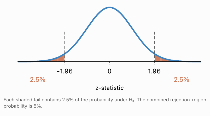
For a two-tailed z-test at α = 0.05, the critical values are:
z = −1.96 and z = +1.96.
Reject H₀ if:
z < −1.96 or z > +1.96.
Otherwise, fail to reject H₀.
Two-tailed z-test at α = 0.05
Worked Example 4: Using Critical Values
A two-tailed z-test produces:
z = 2.24.
The significance level is:
α = 0.05.
The critical values are ±1.96.
Since:
2.24 > 1.96,
the test statistic lies in the rejection region.
Decision: Reject H₀.
The corresponding two-tailed p-value is approximately 0.0251, which is also below 0.05.
Both approaches give the same decision.
Statistical Power and Type II Errors
The probability of a Type II error is represented by:
β (beta)
Statistical power is defined as:
Power = 1 − β
Power is the probability that a test correctly rejects H₀ when a specified alternative is true.
For example:
If β = 0.20,
Power = 1 − 0.20
= 0.80
= 80%.
This means that, if the specified alternative were true, the test would reject H₀ in approximately 80% of repeated studies.
The remaining 20% would result in Type II errors.
Unlike α, β is not usually a single fixed number for every false value of H₀. It depends on the actual effect size and other features of the study.
Factors Affecting Statistical Power
Power generally increases when:
-
Sample size increases.
-
The true effect is larger.
-
Population variability decreases.
-
The significance level is increased, all else equal.
-
The statistical design and measurement process become more efficient.
A test with low power may fail to detect effects that genuinely exist.
Worked Example 5: Calculating Power
A study has a Type II error probability of:
β = 0.15.
Calculate its power.
Power = 1 − β
= 1 − 0.15
= 0.85.
Answer: 85% power.
For the specified alternative, the test has an 85% probability of correctly rejecting H₀.
Worked Example 6: Understanding a Low-Power Study
A researcher investigates whether a new learning programme improves mean test scores.
The study has only eight participants and high variation in student performance.
The test produces:
p = 0.18.
At α = 0.05, the researcher fails to reject H₀.
Can the researcher conclude that the programme has no effect?
No.
The small sample and high variability may result in low statistical power.
A genuine improvement could exist but remain undetected.
A better conclusion is:
"There is insufficient evidence from this study to conclude that the programme improves mean test scores."
A larger, well-designed study could provide a more precise estimate.
The Trade-Off Between Type I and Type II Errors
When sample size and other study conditions remain fixed, lowering α generally reduces the probability of a Type I error but increases the probability of a Type II error for a specified alternative.
Consider a right-tailed z-test of:
H₀: μ = 100
H₁: μ > 100.
Suppose the standard error is 5.
The sample mean must exceed a critical value before H₀ is rejected.
At α = 0.10:
Critical z ≈ 1.282.
Critical sample mean:
100 + 1.282 × 5 = 106.41.
At α = 0.05:
Critical z ≈ 1.645.
Critical sample mean:
100 + 1.645 × 5 = 108.23.
At α = 0.01:
Critical z ≈ 2.326.
Critical sample mean:
100 + 2.326 × 5 = 111.63.
As α decreases, the sample mean must be larger before H₀ is rejected.
Interactive Example: Significance and Power
Suppose the true population mean is 110, the null mean is 100, and the standard error is 5. Explore the consequences of changing α for a right-tailed z-test.
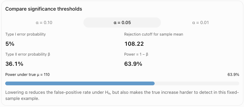
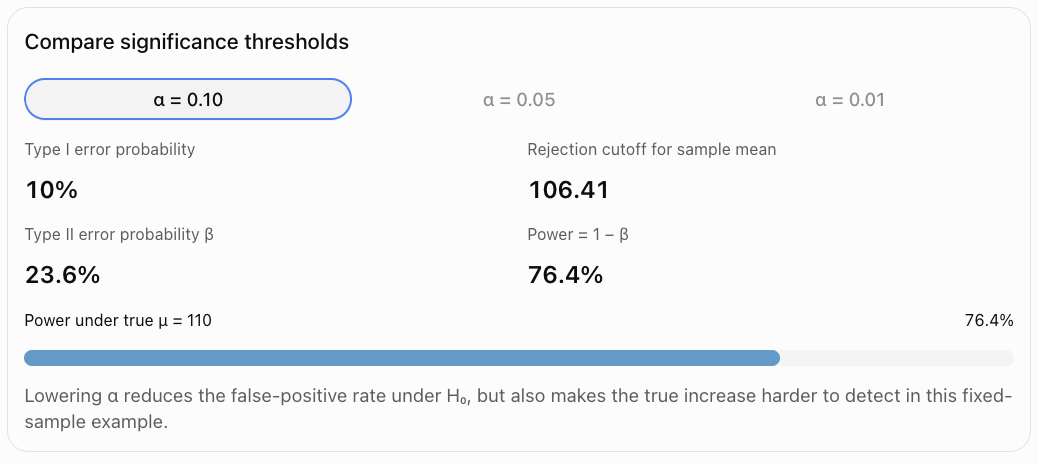
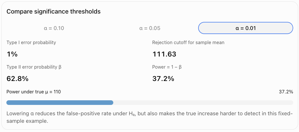
The trade-off can be improved by increasing sample size or reducing measurement variability, rather than simply changing α.
Calculating Type II Error Probability
To calculate β, we need to specify an actual alternative value of the population parameter.
Worked Example 7: Calculating β and Power
A factory tests whether the mean mass of a product exceeds 100 g.
Assume:
H₀: μ = 100 g
H₁: μ > 100 g
Known population standard deviation:
σ = 10 g.
Sample size:
n = 25.
Significance level:
α = 0.05.
Suppose the actual population mean is 105 g.
Calculate β and power.
Step 1: Standard error
SE = σ/√n
= 10/√25
= 2 g.
Step 2: Find the rejection cutoff
For a right-tailed test at α = 0.05:
z* = 1.645.
Reject H₀ when:
x̄ > 100 + 1.645(2)
x̄ > 103.29 g.
Step 3: Calculate β under the true mean of 105 g
A Type II error occurs when the test fails to reject H₀, so:
β = P(x̄ ≤ 103.29 | μ = 105).
Standardize:
z = (103.29 − 105)/2
= −0.855.
Therefore:
β = P(Z ≤ −0.855)
≈ 0.196.
Step 4: Calculate power
Power = 1 − 0.196
= 0.804.
Answer: β ≈ 19.6%, power ≈ 80.4%.
If the true population mean were 105 g, the test would detect the increase in approximately 80.4% of repeated samples.
Worked Example 8: Increasing Sample Size
Keep the same investigation, but increase the sample size from 25 to 100.
Now:
SE = 10/√100 = 1 g.
The rejection cutoff becomes:
100 + 1.645(1) = 101.645 g.
If the true mean is 105 g:
β = P(x̄ ≤ 101.645 | μ = 105).
Standardize:
z = (101.645 − 105)/1
= −3.355.
Thus:
β ≈ 0.0004.
Power ≈ 0.9996
≈ 99.96%.
Conclusion: Increasing sample size from 25 to 100 dramatically increases power to detect a true mean of 105 g, under the assumed model.
However, large sample sizes do not eliminate bias or guarantee practical importance.
Evaluating Statistical Conclusions
A statistical conclusion should be evaluated using more than its p-value.
Researchers should consider the estimated effect, uncertainty, study design, statistical assumptions, and real-world consequences.
Statistical Significance Versus Practical Significance
Statistical significance describes whether the data provide sufficient evidence against H₀ at the chosen α.
Practical significance describes whether the size of the effect matters in the real world.
Worked Example 9: A Statistically Significant but Small Effect
A manufacturer tests whether the mean diameter of a component differs from 20 mm.
A sample of 10,000 components produces:
x̄ = 20.02 mm.
Known σ = 0.5 mm.
H₀: μ = 20
H₁: μ ≠ 20.
Step 1: Standard error
SE = 0.5/√10000
= 0.005 mm.
Step 2: Test statistic
z = (20.02 − 20)/0.005
= 4.00.
Step 3: p-value
For a two-tailed test:
p ≈ 0.000063.
This is statistically significant at α = 0.05.
However, the estimated difference is only 0.02 mm.
Whether that difference matters depends on manufacturing tolerances.
Conclusion: The statistical evidence for a difference is strong, but the practical importance cannot be determined without the engineering requirements.
Confidence Intervals and Statistical Conclusions
Confidence intervals help evaluate the magnitude and precision of estimated effects.
For compatible two-sided procedures:
A 95% confidence interval corresponds to a hypothesis test at α = 0.05.
If the null value lies outside the interval, reject H₀.
If it lies inside the interval, fail to reject H₀.
Worked Example 10: Using a Confidence Interval
A study estimates a mean improvement of 3.5 marks.
The 95% confidence interval for the population mean improvement is:
(0.8, 6.2) marks.
Test:
H₀: μ_d = 0
H₁: μ_d ≠ 0.
Because zero is outside the interval, reject H₀ at α = 0.05, assuming the interval and test are compatible.
There is statistically significant evidence of a nonzero mean improvement.
However, the plausible improvement ranges from 0.8 to 6.2 marks.
If an improvement of at least 5 marks is required to justify the cost of the programme, the interval does not establish that the improvement meets that practical threshold.
Evaluating a Nonsignificant Result
A nonsignificant result does not establish that there is no effect.
Consider two studies.
Study A: Estimated effect = 0.2 marks, 95% CI = (−0.3, 0.7).
Study B: Estimated effect = 0.2 marks, 95% CI = (−8.0, 8.4).
Both intervals contain zero, so neither produces a significant result at the corresponding two-sided 5% level.
However, they tell different stories.
Study A estimates the effect relatively precisely and suggests that large effects are unlikely.
Study B is highly uncertain and remains compatible with both substantial harm and substantial benefit.
Therefore, absence of statistically significant evidence is not the same as evidence of absence.
To establish that an effect is small enough to be practically negligible, researchers may use equivalence tests with predefined equivalence margins.
Worked Example 11: Evaluating Two Studies
A researcher wants to know whether a new teaching programme changes mean test scores by at least 5 marks.
Two studies produce the following results:
|
Study A |
Study B |
|
|---|---|---|
|
Estimated change |
+1 mark |
+1 mark |
|
95% CI |
(0.2, 1.8) |
(−7, 9) |
|
Statistical significance versus zero |
Significant |
Not significant |
Study A: There is evidence of a positive mean change, but the entire confidence interval is below 5 marks. The estimated effect is unlikely to reach the practical target under the model.
Study B: There is insufficient evidence of a nonzero mean change, but the interval includes changes greater than 5 marks. The study is too imprecise to rule out a practically important improvement.
The two studies should not be described simply as one successful and one unsuccessful. Their estimates and uncertainties must be interpreted.
Limitations of Hypothesis Testing
Sampling Bias
If the sample does not represent the target population, statistical results may be misleading.
A small p-value cannot correct a biased sampling process.
Measurement Error
Poorly calibrated instruments, inaccurate self-reporting, or inconsistent procedures can distort results.
Violated Statistical Assumptions
Tests may require independent observations, particular distributional conditions, or sufficiently large samples.
Violating these assumptions can make p-values and error rates unreliable.
Low Statistical Power
A small study may fail to detect a real effect.
A nonsignificant result from a low-power study should be interpreted cautiously.
Multiple Hypothesis Testing
When many tests are performed, the probability of obtaining at least one false positive increases.
If 20 independent tests are performed at α = 0.05 and all null hypotheses are true, the probability of at least one false rejection is:
P(at least one false positive) = 1 − (1 − 0.05)²⁰
= 1 − 0.95²⁰
≈ 0.642.
Answer: Approximately 64.2%.
The calculation assumes independent tests. Dependence changes the exact probability, but multiple testing remains an important concern.
Methods such as the Bonferroni correction and false discovery rate procedures can help manage multiple-testing errors.
Selective Reporting
If researchers report only statistically significant results and omit nonsignificant findings, the published evidence may be distorted.
p-Hacking
Repeatedly changing analyses, excluding observations without a justified plan, or testing many alternatives until p < 0.05 can increase false-positive risk.
Confounding Variables
An observed association may be influenced by other variables.
For example, students who participate in optional tutoring may have higher scores because of differences in motivation or prior achievement.
A significant result alone does not establish causation.
Model Dependence
Statistical conclusions depend on the chosen model.
An incorrect model may produce misleading estimates and significance tests.
Generalizability
A result obtained from one group or setting may not apply to other populations.
Worked Example 12: Multiple Testing
A researcher tests 20 unrelated outcomes at α = 0.05.
Assume all 20 null hypotheses are true and the tests are independent.
The probability that none produces a Type I error is:
0.95²⁰ ≈ 0.3585.
Therefore, the probability of at least one false positive is:
1 − 0.3585
≈ 0.6415.
Answer: Approximately 64.2%.
This does not mean that 64.2% of the tests will be false positives. It means that the probability of getting at least one false positive across the 20 tests is approximately 64.2%.
Real-World Applications
Medical research
Researchers balance the risks of falsely detecting treatment effects and failing to detect genuine benefits or harms.
Manufacturing
Quality-control decisions balance unnecessary production interruptions against missed defects.
Education
Schools evaluate interventions while considering sample size, uncertainty, and practical improvements.
Environmental monitoring
Statistical testing helps identify changes in environmental conditions, while missed problems may have serious consequences.
Integrated Investigation: Evaluating a New Teaching Programme
A school wants to determine whether a new mathematics programme improves average test scores.
The historical mean score is 70 marks.
A random sample of 36 students enrolled in the programme has:
x̄ = 74 marks
s = 12 marks.
Assume a one-sample t-test is appropriate.
Step 1: Hypotheses
H₀: μ = 70
H₁: μ > 70.
Step 2: Significance Level
α = 0.05.
Step 3: Standard Error
SE = 12/√36
= 2 marks.
Step 4: Test Statistic
t = (74 − 70)/2
= 2.00.
Degrees of freedom:
df = 35.
Step 5: p-Value
For a right-tailed t-test with t = 2.00 and df = 35:
p ≈ 0.0266.
Step 6: Statistical Decision
0.0266 < 0.05.
Reject H₀.
Step 7: Statistical Conclusion
There is statistically significant evidence at the 5% level that the population mean score among students enrolled in the programme exceeds 70 marks.
Step 8: Possible Errors
Type I error: Concluding that the population mean score exceeds 70 when it is actually 70.
Type II error: Failing to detect a genuine increase above 70. This study rejected H₀, so a Type II error was not the decision made.
Step 9: Evaluate the Conclusion
The result is statistically significant, but several questions remain:
-
Were the students representative of the target population?
-
Did students volunteer for the programme?
-
Were the tests comparable to the historical assessments?
-
Was the estimated improvement large enough to justify the programme's cost?
-
Could other changes explain the higher scores?
Without random assignment or another credible causal design, the test does not prove that the programme caused the improvement.
Overall conclusion: The evidence suggests a higher population mean score among programme participants, but the causal and practical conclusions require additional investigation.
Common Mistakes
-
Confusing Type I and Type II errors: Type I means rejecting a true H₀; Type II means failing to reject a false H₀.
-
Assuming a rejected H₀ must be false: A Type I error remains possible.
-
Assuming failure to reject proves H₀: The test may lack sufficient power.
-
Interpreting α as the probability that H₀ is true: α controls the false-rejection probability under H₀.
-
Assuming β always equals 1 − α: β depends on the alternative, sample size, variability, and test.
-
Confusing statistical significance with practical importance: A tiny effect can be statistically significant.
-
Interpreting p = 0.03 as a 3% probability that H₀ is true: This is not the meaning of a p-value.
-
Changing α after examining results: This undermines the integrity of the decision procedure.
-
Assuming a larger α is always better: It generally increases power but also increases Type I error risk.
-
Assuming a smaller α eliminates errors: It reduces false-positive risk but can increase false negatives.
-
Ignoring sample size: Small samples may have low power.
-
Ignoring effect size: The magnitude of a difference matters.
-
Ignoring confidence intervals: A p-value alone does not adequately communicate precision.
-
Treating a nonsignificant result as proof of equivalence: Equivalence requires an appropriate design and test.
-
Assuming large samples eliminate bias: A large biased sample can produce misleading results.
-
Ignoring multiple comparisons: Repeated testing increases the opportunity for false-positive findings.
-
Assuming statistical significance establishes causation: Confounding and selection bias may explain associations.
-
Overlooking assumptions: Incorrect assumptions can invalidate nominal error rates.
-
Reporting only significant findings: Selective reporting distorts the evidence.
-
Using absolute language: Statistical conclusions should acknowledge uncertainty and limitations.
Key Terms
-
Hypothesis Test: A statistical procedure for evaluating a claim about a population.
-
Null Hypothesis (H₀): The reference hypothesis tested against the data.
-
Alternative Hypothesis (H₁): The competing claim for which evidence is sought.
-
Type I Error: Rejecting H₀ when H₀ is true.
-
Type II Error: Failing to reject H₀ when H₀ is false.
-
False Positive: A positive conclusion when the tested null condition is actually true.
-
False Negative: A failure to detect an effect that genuinely exists.
-
Significance Level (α): The selected upper bound on the Type I error probability.
-
Beta (β): The Type II error probability under a specified alternative.
-
Statistical Power: The probability of correctly rejecting H₀ under a specified alternative.
-
p-Value: The probability, under H₀ and the model, of a test statistic at least as extreme as the observed one.
-
Statistical Significance: Meeting the chosen criterion for rejecting H₀.
-
Practical Significance: The real-world importance of an estimated effect.
-
Effect Size: A numerical measure of the magnitude of an effect.
-
Test Statistic: A value summarizing how strongly the sample conflicts with H₀.
-
Critical Value: A cutoff used to define a rejection region.
-
Rejection Region: Test-statistic values that lead to rejection of H₀.
-
Standard Error: A measure of the sampling variability of a statistic.
-
Confidence Interval: An interval estimate constructed using a procedure with a specified coverage rate.
-
Sampling Variability: Natural differences between statistics from different samples.
-
Sampling Bias: Systematic distortion caused by an unrepresentative sampling process.
-
Measurement Error: Inaccuracy in observed or recorded values.
-
Confounding Variable: A variable that distorts an apparent relationship between other variables.
-
Multiple Testing: Conducting several statistical tests within an investigation.
-
Familywise Error Rate: The probability of making at least one Type I error across a family of tests.
-
Bonferroni Correction: A method for controlling familywise error by adjusting individual test thresholds.
-
False Discovery Rate: The expected proportion of false rejections among rejected hypotheses, under the relevant procedure's conditions.
-
p-Hacking: Manipulating or selectively exploring analyses to obtain significant results.
-
Selective Reporting: Reporting results based on whether they support a preferred conclusion.
-
Equivalence Testing: Testing whether an effect lies within predefined practically negligible bounds.
-
Generalizability: The extent to which study conclusions apply to a wider population.
-
Statistical Assumption: A condition required for a method's validity.
Key Takeaways
-
Hypothesis tests can produce correct or incorrect decisions.
-
A Type I error occurs when a true null hypothesis is rejected.
-
A Type II error occurs when a false null hypothesis is not rejected.
-
The significance level α controls the Type I error risk under the null model.
-
The probability β measures Type II error risk for a specified alternative.
-
Statistical power equals 1 − β.
-
Increasing sample size generally improves power.
-
Lowering α generally reduces Type I errors but can increase Type II errors.
-
A small p-value provides evidence against H₀, not certainty that H₀ is false.
-
A large p-value does not prove that H₀ is true.
-
Statistical significance does not necessarily mean practical importance.
-
Effect sizes and confidence intervals improve statistical interpretation.
-
Low-power studies may fail to detect genuine effects.
-
A nonsignificant result is not proof of no effect.
-
Multiple testing can increase false-positive risk.
-
Biased sampling can undermine statistical conclusions.
-
Violated model assumptions can make reported p-values unreliable.
-
Statistical association does not automatically establish causation.
-
Conclusions should identify uncertainty, assumptions, and limitations.
-
Good statistical reasoning requires evaluating the evidence, not merely comparing p with 0.05.
Check Your Understanding
Question 1: Identifying Errors
A factory tests whether the mean mass of its products differs from 250 g.
Explain what Type I and Type II errors would mean in this situation.
Question 2: Statistical Significance
A hypothesis test produces p = 0.043.
Determine the decision at α = 0.05 and explain what the result means.
Question 3: Significance Levels
A researcher obtains p = 0.018.
Determine the decision at α = 0.05 and α = 0.01.
Question 4: Calculating Power
A hypothesis test has β = 0.25.
Calculate the power and interpret it.
Question 5: Comparing Error Probabilities
Explain why reducing α from 0.05 to 0.01 may increase the probability of a Type II error when sample size and other conditions remain fixed.
Question 6: Critical Values
A two-tailed z-test at α = 0.05 produces z = −2.31.
Determine the statistical decision using critical values.
Question 7: Practical Significance
A study with 20,000 participants finds an average improvement of 0.1 marks with p = 0.002.
Explain why the result is statistically significant but may not be practically important.
Question 8: Low Statistical Power
A small study finds p = 0.23.
Can the researcher conclude that the intervention has no effect? Explain.
Question 9: Evaluating Confidence Intervals
Two studies investigate the same population mean difference.
Study A: 95% CI = (0.2, 1.4).
Study B: 95% CI = (−5, 7).
Explain which study provides more precise evidence and what each interval suggests about a difference from zero.
Question 10: Multiple Testing
A researcher performs 10 independent hypothesis tests at α = 0.05.
Assuming all null hypotheses are true, calculate the probability of at least one Type I error.
Question 11: Calculating a Type II Error Probability
A right-tailed z-test uses:
H₀: μ = 50
H₁: μ > 50
σ = 12
n = 36
α = 0.05.
Suppose the true population mean is 54.
Calculate the rejection cutoff, β, and power.
Use z* = 1.645.
Question 12: Statistical Conclusions
A researcher obtains p = 0.08 at α = 0.05 and writes:
"The experiment proves that the treatment has no effect."
Explain why this conclusion is incorrect and provide a better statement.
Question 13: Sampling Bias
A school surveys only students in an advanced mathematics class to estimate the average mathematics achievement of all students.
Explain how sampling bias may affect the hypothesis test.
Question 14: Error Consequences
A public health researcher tests whether a pollutant exceeds a specified safety threshold.
Explain why Type I and Type II errors may have different consequences.
Question 15: Comprehensive Evaluation
A school investigates whether a new study programme increases average mathematics scores above a historical mean of 70 marks.
A random sample of 64 programme participants has:
x̄ = 72.5
Known σ = 10
α = 0.05.
Assume a one-sample z-test is appropriate.
Calculate and explain:
a) H₀ and H₁.
b) The standard error.
c) The z-test statistic.
d) The p-value.
e) The statistical decision.
f) The Type I error in context.
g) The Type II error in context.
h) Whether the result proves that the programme caused an improvement.
i) Two limitations of the study.
Fully Worked Answers
Answer 1: Identifying Errors
The hypotheses are:
H₀: μ = 250 g
H₁: μ ≠ 250 g.
Type I error: Concluding that the population mean mass differs from 250 g when it is actually 250 g.
Type II error: Failing to reject H₀ when the true population mean differs from 250 g.
The first could cause unnecessary changes to production. The second could allow a real manufacturing problem to remain undetected.
Answer 2: Statistical Significance
Given:
p = 0.043
α = 0.05.
Since:
0.043 < 0.05,
reject H₀.
Conclusion: The result is statistically significant at the 5% level.
The data provide sufficient evidence against H₀ according to the selected test, but they do not establish that the alternative hypothesis is certainly true.
Answer 3: Significance Levels
p = 0.018.
At α = 0.05:
0.018 < 0.05.
Reject H₀.
At α = 0.01:
0.018 > 0.01.
Fail to reject H₀.
The same evidence produces different decisions because the thresholds differ.
Answer 4: Calculating Power
Given:
β = 0.25.
Power = 1 − β
= 1 − 0.25
= 0.75.
Answer: 75% power.
For the specified alternative, the test has a 75% probability of correctly rejecting H₀.
Answer 5: Comparing Error Probabilities
Reducing α from 0.05 to 0.01 makes the rejection criterion stricter.
The observed result must be more extreme before H₀ is rejected.
This reduces the probability of rejecting a true H₀.
However, when H₀ is false, some results that would previously have led to rejection may now lead to failure to reject.
Therefore, β generally increases and power decreases when other conditions remain fixed.
Answer 6: Critical Values
Given:
z = −2.31.
For a two-tailed z-test at α = 0.05:
Critical values = ±1.96.
Since:
−2.31 < −1.96,
the statistic lies in the left rejection region.
Decision: Reject H₀.
The result is statistically significant at the 5% level.
Answer 7: Practical Significance
Given:
p = 0.002.
Since p < 0.05, the result is statistically significant.
However, the estimated improvement is only 0.1 marks.
A very large sample can detect extremely small differences.
The improvement may not justify the cost, time, or effort required to implement the intervention.
Conclusion: The statistical evidence of a difference is strong, but its practical importance may be negligible.
Answer 8: Low Statistical Power
No.
A p-value of 0.23 means that the result is not statistically significant at α = 0.05.
However, a small sample may have insufficient power to detect a real effect.
A suitable conclusion is:
"There is insufficient statistical evidence from this study to conclude that the intervention has an effect."
The researcher should consider the effect estimate, confidence interval, and statistical power.
Answer 9: Evaluating Confidence Intervals
Study A: (0.2, 1.4)
The interval is relatively narrow and excludes zero.
For a compatible two-sided 5% test, this indicates a statistically significant positive population mean difference.
Study B: (−5, 7)
The interval is much wider and includes zero.
It is compatible with substantial negative effects, no effect, and substantial positive effects.
Conclusion: Study A provides more precise evidence. Study B has much greater uncertainty.
Answer 10: Multiple Testing
Given:
10 independent tests.
α = 0.05.
Assume all null hypotheses are true.
Probability of no Type I errors:
P(no errors) = 0.95¹⁰
≈ 0.5987.
Probability of at least one Type I error:
P(at least one) = 1 − 0.5987
≈ 0.4013.
Answer: Approximately 40.1%.
This is the probability of at least one false positive across the ten tests, not the expected percentage of tests that are false positives.
Answer 11: Calculating Type II Error Probability
Given:
H₀: μ = 50
H₁: μ > 50
σ = 12
n = 36
α = 0.05
True mean = 54.
Step 1: Standard error
SE = 12/√36
= 2.
Step 2: Rejection cutoff
Critical sample mean:
50 + 1.645 × 2
= 53.29.
Reject H₀ when:
x̄ > 53.29.
Step 3: Calculate β
When the true mean is 54:
β = P(x̄ ≤ 53.29 | μ = 54).
Standardize:
z = (53.29 − 54)/2
= −0.355.
From the standard normal distribution:
β ≈ 0.3613.
Step 4: Calculate power
Power = 1 − 0.3613
= 0.6387.
Answers:
-
Rejection cutoff = 53.29.
-
β ≈ 36.1%.
-
Power ≈ 63.9%.
The test would detect the specified increase to 54 in approximately 63.9% of repeated samples.
Answer 12: Statistical Conclusions
The researcher's statement is incorrect because failing to reject H₀ does not prove that the null hypothesis is true.
Given:
p = 0.08
α = 0.05.
Since p > α, fail to reject H₀.
A better conclusion is:
"At the 5% significance level, there is insufficient statistical evidence that the treatment has an effect."
A confidence interval would help determine which effect sizes remain plausible.
Answer 13: Sampling Bias
Students in advanced mathematics classes may have higher mathematics achievement than the general student population.
Therefore, their scores may not represent all students.
The sample could systematically overestimate the population mean.
A hypothesis test based on this sample may produce a misleading conclusion, even if the p-value is very small.
A more appropriate approach would use a representative random sample from the full student population.
Answer 14: Error Consequences
Suppose:
H₀: μ = safety threshold
H₁: μ > safety threshold.
Type I error: Concluding that the population mean pollutant concentration exceeds the threshold when the null value is actually correct.
This may cause unnecessary warnings, closures, or interventions.
Type II error: Failing to detect a true exceedance of the safety threshold.
This may expose people or ecosystems to a genuine environmental hazard.
Because the consequences differ, the significance level and required power should be chosen with the decision context in mind.
Answer 15: Comprehensive Evaluation
Given:
x̄ = 72.5
μ₀ = 70
σ = 10
n = 64
α = 0.05.
a) Hypotheses
H₀: μ = 70.
H₁: μ > 70.
This is a right-tailed test.
b) Standard error
SE = σ/√n
= 10/√64
= 10/8
= 1.25 marks.
c) z-test statistic
z = (72.5 − 70)/1.25
= 2.5/1.25
= 2.00.
d) p-value
For a right-tailed test:
p = P(Z ≥ 2.00)
≈ 0.0228.
e) Statistical decision
0.0228 < 0.05.
Reject H₀.
There is statistically significant evidence that the population mean score among programme participants exceeds 70 marks.
f) Type I error
Concluding that the population mean score exceeds 70 when the true population mean is actually 70.
g) Type II error
Failing to reject H₀ when the true population mean score exceeds 70.
Although this particular test rejected H₀, Type II errors remain an important consideration when designing similar studies.
h) Does the result prove causation?
No.
The sample mean is higher than the historical benchmark, and the difference is statistically significant.
However, the students may differ from previous students in motivation, preparation, or other characteristics.
Without an appropriate comparison design, the result does not establish that the programme caused the increase.
i) Two limitations
-
Selection bias: Students participating in the programme may not represent the wider student population.
-
Historical comparison: The historical mean may come from a different cohort or assessment conditions, making direct comparison unreliable.
A randomized controlled study, or another carefully designed comparison, would provide stronger evidence about the programme's causal effect.
Final Course Connections
Errors in statistical testing are a central part of statistical inference because every decision based on a sample involves uncertainty.
Type I errors represent false rejections, while Type II errors represent missed genuine effects. Significance levels control one kind of risk, and statistical power describes the ability to detect specified alternatives.
Understanding these concepts helps researchers make more responsible decisions. Rather than focusing only on whether p is below 0.05, a strong statistical analysis considers effect sizes, confidence intervals, sample quality, study design, assumptions, and real-world consequences.
The most important principle is that statistical significance is evidence, not certainty, and a statistically nonsignificant result is not proof that no effect exists.
This completes Errors in Statistical Testing, covering all five learning targets with 12 worked examples, visual explanations, an interactive significance-and-power comparison, real-world applications, common mistakes, key terms, key takeaways, and 15 practice questions with fully worked answers.