Box Plots and Histograms

Introduction

Statistical graphs help us understand how data are organised, distributed, and spread out.

Two particularly useful graphs are box plots and histograms.

A box plot summarises a dataset using its median, quartiles, and overall spread. It is especially useful for comparing different datasets and identifying potential outliers.

A histogram shows how frequently numerical values occur within intervals. It is especially useful for identifying the shape of a distribution, including symmetry, skewness, clusters, and gaps.

Although both graphs describe distributions, they reveal different information.

For example, a histogram can show whether examination scores form one peak or two, while a box plot makes it easier to compare the medians and interquartile ranges of two classes.

Understanding how to construct and interpret these graphs allows us to draw meaningful conclusions from data.

Understanding Box Plots

A box plot, also called a box-and-whisker plot, is a graph that summarises the centre and spread of numerical data.

A traditional box plot is constructed using five important values, called the five-number summary:

• Minimum

• First quartile (Q₁)

• Median (Q₂)

• Third quartile (Q₃)

• Maximum

These values divide the dataset into four sections containing approximately 25% of the observations each.

A modified box plot also identifies potential outliers separately.

The Structure of a Box Plot

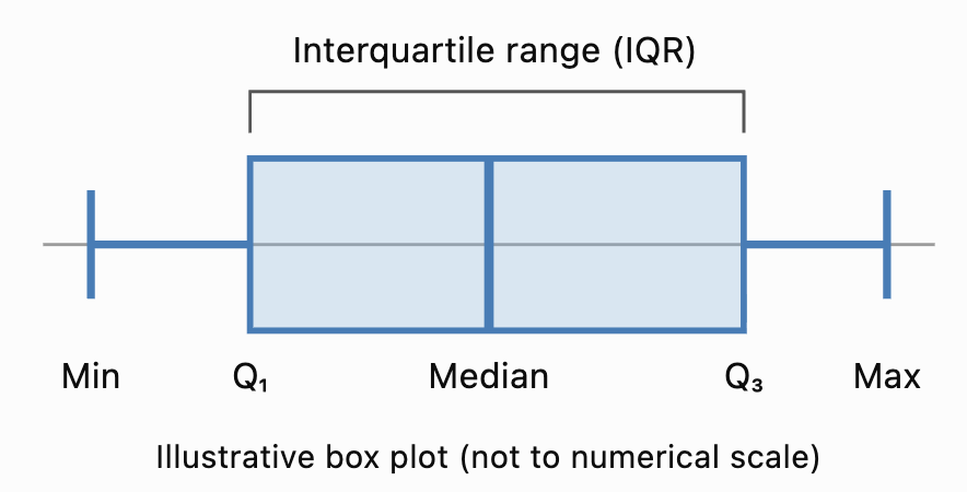
Important Features

The box extends from Q₁ to Q₃.

The line inside the box represents the median.

The length of the box represents the interquartile range.

The whiskers extend toward the lowest and highest values included under the chosen box-plot convention.

In a traditional box plot, the whiskers extend to the minimum and maximum observations.

In a modified box plot, the whiskers extend to the most extreme observations that are not classified as outliers.

The Five-Number Summary

Before constructing a box plot, we need to calculate the five-number summary.

Consider the ordered dataset:

3, 5, 7, 8, 10, 12, 14, 16, 18, 21, 25

Minimum

The smallest value is:

Minimum = 3

Maximum

The largest value is:

Maximum = 25

Median

There are 11 observations.

The median is the sixth value.

Median = 12

First Quartile

Using the median-of-halves method, exclude the median and examine the lower five values:

3, 5, 7, 8, 10

The middle value is 7.

Q₁ = 7

Third Quartile

Examine the upper five values:

14, 16, 18, 21, 25

The middle value is 18.

Q₃ = 18

Five-Number Summary

This summary provides the information needed to construct a traditional box plot.

Note: Several accepted quartile conventions exist. These notes use the median-of-halves method, excluding the overall median when the dataset has an odd number of observations. Other methods may produce slightly different quartiles.

Constructing a Box Plot

Let's construct a box plot for:

4, 6, 8, 10, 12, 14, 16, 18, 20

Step 1: Order the Data

The values are already arranged in ascending order.

Step 2: Identify the Minimum and Maximum

Minimum = 4

Maximum = 20

Step 3: Find the Median

There are nine observations.

The fifth value is 12.

Median = 12

Step 4: Find the Quartiles

Lower half:

4, 6, 8, 10

Q₁ = (6 + 8)/2 = 7

Upper half:

14, 16, 18, 20

Q₃ = (16 + 18)/2 = 17

Step 5: Record the Five-Number Summary

Step 6: Draw a Number Line

Choose a suitable horizontal scale covering the data.

For this example, a scale from 0 to 22 is appropriate.

Step 7: Draw the Box

Draw a rectangle extending from Q₁ = 7 to Q₃ = 17.

Step 8: Mark the Median

Draw a vertical line inside the box at 12.

Step 9: Add the Whiskers

Draw lines extending from the box to the minimum and maximum.

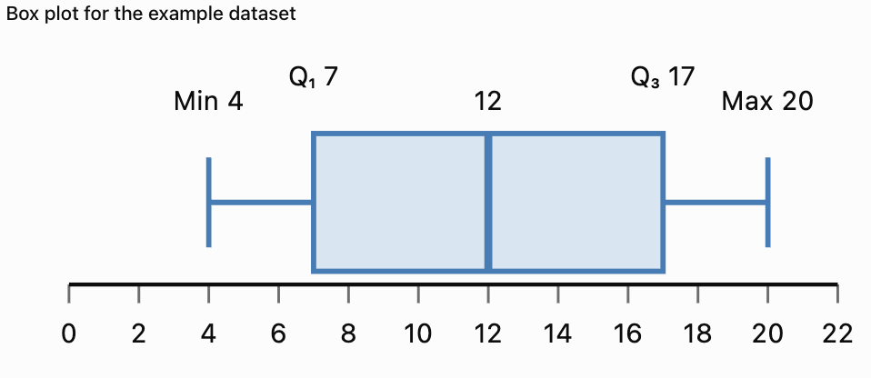
The completed box plot shows the centre and spread of the dataset.

Understanding the Interquartile Range

The interquartile range (IQR) measures the spread of the middle 50% of the observations.

The formula is:

IQR = Q₃ − Q₁

For the previous dataset:

Q₁ = 7

Q₃ = 17

IQR = 17 − 7

IQR = 10

Interpretation

The middle 50% of the observations lie between 7 and 17.

The width of this interval is 10 units.

A smaller IQR indicates that the middle half of the data is more closely grouped.

A larger IQR indicates that the middle half is more widely spread.

Why Is the IQR Useful?

The IQR is resistant to extreme values.

Unlike the range, it is not determined by the smallest and largest observations.

This makes it particularly useful for skewed distributions or datasets containing outliers.

Identifying Outliers Using Box Plots

An outlier is an observation unusually far from the main group of data.

A common method for identifying potential outliers uses the IQR.

Outlier Fences

Lower fence = Q₁ − 1.5 × IQR

Upper fence = Q₃ + 1.5 × IQR

Observations below the lower fence or above the upper fence are flagged as potential outliers.

Worked Example

Consider:

5, 6, 7, 8, 9, 10, 11, 12, 13, 40

Step 1: Find the Median

Median = (9 + 10)/2

Median = 9.5

Step 2: Find Q₁ and Q₃

Lower half:

5, 6, 7, 8, 9

Q₁ = 7

Upper half:

10, 11, 12, 13, 40

Q₃ = 12

Step 3: Calculate the IQR

IQR = 12 − 7

IQR = 5

Step 4: Calculate the Fences

Lower fence = 7 − 1.5(5)

Lower fence = −0.5

Upper fence = 12 + 1.5(5)

Upper fence = 19.5

Step 5: Identify Outliers

The value 40 exceeds the upper fence.

40 is a potential outlier.

Modified Box Plot

In a modified box plot:

• The box extends from Q₁ = 7 to Q₃ = 12.

• The median is 9.5.

• The lower whisker extends to 5.

• The upper whisker extends to 13.

• The outlier 40 is shown separately as a point.

Important Observation

An outlier is not necessarily an error.

It may represent a genuine unusual event, an extreme measurement, or a mistake.

Outliers should be investigated before deciding whether they should be excluded.

Interpreting Box Plot Shapes

Box plots can provide clues about the shape of a distribution.

Approximately Symmetric Distribution

In an approximately symmetric distribution:

• The median is often near the centre of the box.

• The whiskers may have similar lengths.

• The two halves of the box may be similar in width.

Right-Skewed Distribution

A right-skewed distribution may have:

• A longer upper whisker.

• A median closer to Q₁.

• High-value outliers.

Left-Skewed Distribution

A left-skewed distribution may have:

• A longer lower whisker.

• A median closer to Q₃.

• Low-value outliers.

Important Limitation

Box plots provide clues about skewness but do not show the complete distribution.

A histogram is generally better for examining detailed distribution shape and identifying multiple peaks.

Comparing Multiple Box Plots

One of the main advantages of box plots is that several datasets can be compared on the same numerical scale.

Suppose two classes complete a mathematics examination.

Class A

50, 55, 60, 65, 70, 75, 80, 85, 90

Class B

40, 45, 50, 65, 70, 75, 90, 95, 100

Calculate the Five-Number Summaries

Interpretation

Both classes have the same median score of 70.

However, Class B has a larger IQR and range.

This means the scores in Class B are more widely spread.

Class A has more consistent scores around the centre.

What Should We Compare?

When comparing box plots, examine:

• Median: Which group has the higher typical value?

• IQR: Which group has more variation in its middle 50%?

• Range: Which group has the greater overall spread?

• Outliers: Are there unusual observations?

• Shape: Are the quartile intervals and whiskers balanced?

Understanding Histograms

A histogram is a graph that displays the frequency distribution of numerical data.

Histograms group values into intervals called bins or classes.

The horizontal axis shows the numerical intervals.

The vertical axis usually shows frequency.

The bars touch because adjacent intervals represent consecutive parts of a numerical scale.

Example

A teacher records the examination scores of 30 students.

A histogram makes it easier to see where scores are concentrated.

Most students scored between 60 and 79.

Constructing a Histogram

Consider the following 20 measurements:

12, 15, 17, 18, 21, 22, 24, 25, 27, 28, 31, 32, 33, 35, 36, 38, 41, 43, 45, 48

Step 1: Identify the Range

Minimum = 12

Maximum = 48

Range = 48 − 12

Range = 36

Step 2: Choose Intervals

We will use equal-width intervals of 10 units.

• 10–19

• 20–29

• 30–39

• 40–49

For integer data, these can be treated as intervals 10 ≤ x < 20, 20 ≤ x < 30, and so on.

Step 3: Count the Frequencies

Step 4: Draw the Axes

Label the horizontal axis with the measurement intervals.

Label the vertical axis with frequency.

Step 5: Draw the Bars

Each bar represents the frequency of its interval.

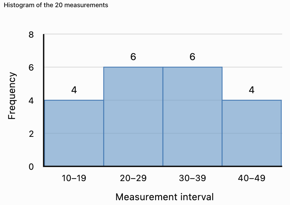
Interpretation

The middle intervals have the highest frequencies.

The frequencies are balanced around the centre.

The distribution appears approximately symmetric.

Histograms Versus Bar Charts

Histograms and bar charts may look similar, but they represent different types of data.

Example

A histogram might display the heights of 100 students.

A bar chart might display how many students prefer Mathematics, Science, English, or History.

Choosing Histogram Intervals

The choice of interval width affects the appearance of a histogram.

Very Wide Intervals

Wide intervals produce fewer bars.

They may hide important details such as gaps or multiple peaks.

Very Narrow Intervals

Narrow intervals produce more bars.

They may reveal additional detail but can make the graph appear irregular.

Appropriate Intervals

A useful histogram should have intervals that:

• Cover the entire dataset.

• Do not overlap.

• Have clearly defined boundaries.

• Are usually equal in width.

• Reveal meaningful patterns.

There is no single best interval width for every dataset.

Example

Suppose test scores range from 0 to 100.

Using intervals of width 50 creates only two bars.

Using intervals of width 10 creates ten bars.

The second histogram may reveal more detail about the shape of the distribution.

Unequal Histogram Intervals

Sometimes histograms use intervals of different widths.

In these cases, using frequency directly as bar height can be misleading.

Instead, the bar height should represent frequency density.

Frequency Density Formula

Frequency density = Frequency / Class width

The area of each bar then represents the frequency.

Worked Example

Interpretation

The interval 20–40 has the highest total frequency, but it is twice as wide as the first two intervals.

Its frequency density is therefore 2.

A histogram with unequal intervals must account for the different widths.

Remember: For unequal-width histograms, bar area—not bar height alone—represents frequency.

Interpreting Histogram Shapes

Histograms reveal important patterns in numerical data.

Symmetric Distribution

A symmetric histogram has approximately balanced sides.

The frequencies often increase toward the centre and decrease toward both ends.

Right-Skewed Distribution

A right-skewed histogram has a longer tail toward larger values.

Most observations are concentrated toward the lower end.

Left-Skewed Distribution

A left-skewed histogram has a longer tail toward smaller values.

Most observations are concentrated toward the higher end.

Unimodal Distribution

A unimodal distribution has one main peak.

Bimodal Distribution

A bimodal distribution has two main peaks.

This may indicate that the data contain two distinct groups.

Uniform Distribution

A uniform distribution has approximately equal frequencies across its intervals.

Important Observation

Histograms reveal features that box plots may hide.

For example, a box plot may not show that a dataset has two separate peaks.

Identifying Outliers in Histograms

An outlier may appear as an isolated bar or a small group of observations separated from the main distribution.

Example

Suppose most examination scores are between 50 and 90, but one score is 5.

The histogram may show a gap between the low score and the rest of the distribution.

This suggests that the low score should be investigated.

However, a histogram alone does not establish whether a value meets a formal outlier rule.

The appearance also depends on the chosen intervals.

Box Plots Versus Histograms for Outliers

Box plots can use a formal IQR-based rule to identify potential outliers.

Histograms can reveal isolated observations or unusual gaps.

Both are useful, but they provide different kinds of evidence.

Comparing Multiple Histograms

When comparing histograms, examine the shape, centre, spread, and unusual features.

Suppose two classes complete the same examination.

Class A

Most students score between 60 and 80.

The distribution is approximately symmetric.

Class B

Most students score between 40 and 60, but a few students score above 90.

The distribution is right-skewed.

Interpretation

Class A appears to have more consistent results around the middle.

Class B has a larger concentration of lower scores and a small number of high scores.

However, exact comparisons of centre and spread require numerical summaries or more detailed data.

Fair Comparisons

When comparing histograms, it is helpful to use:

• The same numerical scale.

• The same interval boundaries.

• The same interval widths.

• Relative frequencies when sample sizes differ.

If one class contains 20 students and another contains 200, raw frequency bars may not be directly comparable.

Relative-frequency histograms can solve this problem.

Relative-Frequency Histograms

A relative-frequency histogram shows proportions or percentages rather than raw counts.

Formula

Relative frequency = Frequency / Total observations

To convert to a percentage:

Percentage frequency = (Frequency / Total) × 100%

Worked Example

A class of 40 students receives the following results:

Interpretation

Forty percent of the class scored between 60 and 79.

Relative-frequency histograms are particularly useful when comparing groups of different sizes.

Box Plots and Histograms: Strengths and Limitations

Which Graph Should We Use?

Use a box plot when the goal is to compare medians, quartiles, spreads, and potential outliers.

Use a histogram when the goal is to examine distribution shape, peaks, clusters, and gaps.

Using both graphs together often provides the clearest understanding.

Real-World Application: Examination Results

Teachers can use box plots and histograms to analyse student performance.

Using a Histogram

A histogram can show:

• Whether scores cluster near the middle.

• Whether an examination appears relatively easy or difficult for a group.

• Whether there are two distinct groups of scores.

• Whether a few students have unusually low or high results.

Using a Box Plot

A box plot can show:

• The median score.

• The middle 50% of results.

• Differences in spread between classes.

• Potential outliers.

Interpretation

If two classes have the same median but different IQRs, they have similar central scores but different levels of variability.

The class with the smaller IQR has a more tightly grouped middle half of scores.

Real-World Application: Manufacturing

A factory produces metal components with a target diameter of 20 mm.

A histogram can reveal whether most components are close to the target diameter.

A box plot can compare the spread of measurements from different production machines.

Example

Machine A:

Median diameter = 20.0 mm

IQR = 0.2 mm

Machine B:

Median diameter = 20.0 mm

IQR = 0.8 mm

Both machines have the same median.

However, Machine A has a smaller IQR.

Its middle 50% of measurements are more consistent.

This does not by itself establish whether either machine meets the required tolerances.

Real-World Application: Environmental Measurements

Environmental scientists may use histograms to examine rainfall, temperature, or air-quality measurements.

Rainfall Example

A histogram of daily rainfall may show many days with little rainfall and a few days with very heavy rainfall.

This produces a right-skewed distribution.

A box plot can help identify unusually wet days.

Interpretation

Extreme observations may be important for planning drainage systems, managing flood risk, and understanding environmental variability.

Removing unusual values without investigation could eliminate important information.

Common Mistakes

Forgetting to order data before finding quartiles

Quartiles must be calculated from ordered observations.

Confusing the median with the mean

The line inside a standard box plot represents the median, not necessarily the mean.

Drawing whiskers to outliers in a modified box plot

Modified box plots show potential outliers separately.

Assuming the box represents all observations

The box represents the middle 50% of the distribution.

Confusing IQR with range

IQR = Q₃ − Q₁.

Range = Maximum − Minimum.

Using overlapping histogram intervals

Each observation should belong to exactly one interval.

Leaving gaps between histogram bars

For consecutive numerical intervals, histogram bars normally touch.

Using unequal intervals without frequency density

Unequal-width histograms require bar heights that account for interval widths.

Confusing histogram and bar chart data

Histograms display numerical distributions; bar charts usually compare categories.

Assuming a box plot reveals every feature of the distribution

Box plots do not directly reveal multiple peaks or detailed clusters.

Comparing graphs with different scales carelessly

Different scales can make similar distributions appear very different.

Assuming an isolated bar proves an outlier

Histogram appearance depends on interval selection.

Key Terms

• Box Plot: Graph summarising the centre and spread of numerical data.

• Box-and-Whisker Plot: Another name for a box plot.

• Five-Number Summary: Minimum, Q₁, median, Q₃, and maximum.

• Minimum: Smallest observation.

• Maximum: Largest observation.

• Median: Middle value of ordered data.

• First Quartile (Q₁): Value separating approximately the lowest 25% of observations.

• Third Quartile (Q₃): Value separating approximately the lowest 75% of observations.

• Interquartile Range (IQR): Difference between Q₃ and Q₁.

• Range: Difference between the maximum and minimum.

• Whisker: Line extending from a box toward the extremes of the data under the chosen convention.

• Outlier: Observation unusually far from the main group.

• Lower Fence: Q₁ − 1.5 × IQR.

• Upper Fence: Q₃ + 1.5 × IQR.

• Histogram: Graph displaying the frequency distribution of numerical data.

• Frequency: Number of observations in a category or interval.

• Relative Frequency: Proportion of observations in an interval.

• Class Interval: Numerical interval used to group observations.

• Bin: Another term for a histogram interval.

• Class Width: Numerical width of an interval.

• Frequency Density: Frequency divided by interval width.

• Symmetric Distribution: Distribution with approximately balanced sides.

• Right-Skewed Distribution: Distribution with a longer right tail.

• Left-Skewed Distribution: Distribution with a longer left tail.

• Unimodal Distribution: Distribution with one main peak.

• Bimodal Distribution: Distribution with two main peaks.

• Cluster: Region containing many observations.

• Gap: Region containing few or no observations.

• Spread: Extent to which observations vary.

• Statistical Graph: Visual representation of data.

Key Takeaways

• Box plots summarise numerical data using quartiles, median, and spread.

• The five-number summary includes minimum, Q₁, median, Q₃, and maximum.

• The box represents the middle 50% of the data.

• IQR = Q₃ − Q₁.

• Modified box plots show potential outliers separately.

• Outlier fences can be calculated using 1.5 × IQR.

• Histograms display the frequencies of numerical intervals.

• Histogram bars normally touch.

• Histograms are useful for identifying symmetry, skewness, peaks, gaps, and clusters.

• Equal-width intervals simplify histogram construction.

• Unequal-width histograms require frequency density.

• Box plots are especially useful for comparing centres and spreads.

• Histograms are especially useful for examining distribution shape.

• Relative frequencies allow comparisons between groups of different sizes.

• Using both box plots and histograms provides a more complete understanding of a dataset.

Check Your Understanding

Box Plots

1. What five values make up the five-number summary?

2. What does the line inside a box plot represent?

3. What percentage of observations is represented by the box?

4. Calculate the IQR if Q₁ = 15 and Q₃ = 35.

5. Calculate the range if the minimum is 8 and maximum is 62.

Constructing Box Plots

Use the median-of-halves quartile convention.

6. Find the median of 2, 4, 6, 8, 10, 12, 14.

7. Find Q₁ and Q₃ for the same dataset.

8. Calculate the IQR.

9. Determine the lower and upper outlier fences.

10. Explain how an outlier is displayed on a modified box plot.

Histograms

11. What type of data is displayed in a histogram?

12. Why do histogram bars normally touch?

13. What does the vertical axis usually represent?

14. Explain the difference between a histogram and a bar chart.

15. Why is interval width important?

Comparing Graphs

16. Which graph is better for comparing medians?

17. Which graph is better for identifying two peaks?

18. What does a larger IQR indicate?

19. Why might relative-frequency histograms be useful?

20. Explain one advantage of using both box plots and histograms.

Answer Key

Extended Challenge

Constructing Box Plots

Use the median-of-halves quartile convention.

1. Construct a box plot for 5, 8, 10, 12, 15, 18, 20, 22, 25.

2. Calculate the five-number summary.

3. Determine the IQR.

4. Calculate the outlier fences.

5. Explain whether any observations are potential outliers.

Constructing Histograms

Consider the following data:

12, 15, 18, 21, 24, 25, 28, 31, 33, 35, 38, 40, 42, 45, 48, 51, 53, 55, 58, 60

6. Create a frequency table using intervals of width 10.

7. Construct a histogram.

8. Identify the interval with the greatest frequency.

9. Describe the overall shape of the distribution.

10. Explain how changing the interval width might affect the graph.

Comparing Distributions

Dataset A:

40, 45, 50, 55, 60, 65, 70

Dataset B:

20, 35, 50, 55, 60, 75, 90

11. Calculate the median of each dataset.

12. Calculate the IQR of each dataset.

13. Calculate the range of each dataset.

14. Construct side-by-side box plots.

15. Compare the centres and spreads of the datasets.

Advanced Interpretation

16. Explain why a histogram may reveal bimodality while a box plot does not.

17. Describe how an extreme outlier could affect a box plot.

18. Explain why relative frequencies are useful when comparing classes of different sizes.

19. Describe a situation where a histogram would be more informative than a box plot.

20. Explain why both graphical and numerical summaries are important in statistical analysis.

Final Investigation: Comparing Student Examination Results

Three classes complete the same examination.

Class A

48, 52, 55, 58, 60, 62, 65, 68, 72, 75

Class B

35, 42, 50, 55, 60, 65, 70, 78, 85, 92

Class C

45, 48, 50, 52, 55, 58, 60, 62, 65, 98

Complete the investigation.

1. Order each dataset.

2. Calculate the mean of each class.

3. Calculate the median of each class.

4. Calculate the minimum and maximum.

5. Calculate the range.

6. Find Q₁ and Q₃ using the median-of-halves method.

7. Calculate the IQR.

8. Determine the lower and upper outlier fences.

9. Identify potential outliers.

10. Construct a modified box plot for each class.

11. Display all three box plots on the same numerical scale.

12. Compare the median scores.

13. Compare the IQRs.

14. Identify which class has the greatest overall spread.

15. Construct a frequency table for each class using common score intervals.

16. Draw a histogram for each class using the same interval widths and axes.

17. Describe the shape of each distribution.

18. Identify any clusters, gaps, or unusual observations.

19. Explain which graph provides the clearest information about differences between the classes.

20. Write a statistical report comparing the three classes using evidence from both box plots and histograms.