Descriptive Statistics
| Site: | Young Education |
| Cursus: | Statistics |
| Boek: | Descriptive Statistics |
| Afgedrukt door: | Guest user |
| Datum: | maandag, 9 november 2026, 16:37 |
1. Measures of Centre
Learning outcomes
- I can calculate the mean.
- I can calculate the median.
- I can calculate the mode.
- I can compare measures of centre.
- I can select appropriate measures for different datasets.
Measures of Centre
Introduction
When we collect data, we often want to describe the information using a single number that represents a typical or central value.
For example, imagine that a teacher records the scores of students on a mathematics quiz. Rather than examining every individual score, the teacher might calculate an average to understand how the class performed.
Similarly, a business might want to know the typical amount customers spend, or a scientist might want to determine the typical height of plants in an experiment.
These situations involve measures of centre, also called measures of central tendency.
The three most common measures of centre are:
-
Mean: The sum of all values divided by the number of values.
-
Median: The middle value when data is arranged in order.
-
Mode: The value that occurs most frequently.
Each measure describes the centre of a dataset differently. Understanding these differences helps us select the most appropriate measure for a particular situation.


What Is a Dataset?
A dataset is a collection of values or observations gathered for analysis.
For example, consider the number of books read by eight students during a month:
2, 4, 3, 5, 4, 6, 3, 5
Each number represents one observation.
The dataset contains eight values.
We can use measures of centre to describe a typical number of books read.
Before calculating a measure of centre, it is important to understand the data.
Questions to consider include:
-
How many values are there?
-
Are the values numerical or categorical?
-
Are any values unusually large or small?
-
Are some values repeated?
-
What does each value represent?
The answers help determine which measure of centre is most useful.
The Mean
The mean is calculated by adding all the values in a dataset and dividing by the number of values.
It is often called the arithmetic average.
Formula
Mean = Sum of all values ÷ Number of values
Using mathematical notation:
x̄ = Σx/n
Where:
-
x̄ represents the sample mean.
-
Σx represents the sum of all values.
-
n represents the number of values.
The symbol Σ (sigma) means sum.
Worked Example: Quiz Scores
Five students receive the following quiz scores:
6, 8, 7, 9, 10
Find the mean.
Step 1: Add the values.
6 + 8 + 7 + 9 + 10 = 40
Step 2: Count the values.
There are 5 scores.
Step 3: Divide.
Mean = 40 ÷ 5
Mean = 8
The mean quiz score is 8.
Interpretation
The mean represents an equal-sharing value.
If the total of 40 points were distributed equally among the five students, each would have 8 points.
This does not mean every student actually scored 8.
Understanding the Mean Visually
Consider the dataset:
2, 3, 3, 4, 8
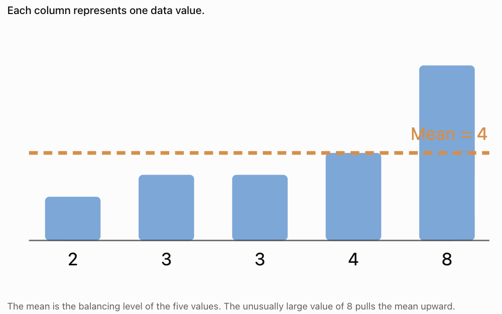
Calculate:
Mean = (2 + 3 + 3 + 4 + 8)/5
= 20/5
Mean = 4
Notice that only one value is greater than 4, but that value is much larger than the others.
This demonstrates how an unusually high value can affect the mean.
Finding the Mean with Decimal Values
The mean can be calculated using whole numbers, decimals, or negative numbers.
Worked Example: Temperatures
A scientist records these temperatures in degrees Celsius:
21.5, 22.0, 23.5, 21.0, 22.5
Calculate the mean.
Add:
21.5 + 22.0 + 23.5 + 21.0 + 22.5 = 110.5
Divide by 5:
Mean = 110.5/5
Mean = 22.1°C
Important Point
The mean does not have to be one of the values in the dataset.
For example, the mean of 3 and 4 is 3.5.
Finding the Mean from a Frequency Table
Sometimes a dataset contains many repeated values.
A frequency table makes it easier to calculate the mean.
Worked Example
The following table shows the number of siblings students have.
|
Number of siblings (x) |
Frequency (f) |
f × x |
|---|---|---|
|
0 |
3 |
0 |
|
1 |
5 |
5 |
|
2 |
4 |
8 |
|
3 |
2 |
6 |
|
Total |
14 |
19 |
The mean is:
Mean = Σ(f × x)/Σf
Substitute:
Mean = 19/14
Mean ≈ 1.36 siblings
Interpretation
The average number of siblings is approximately 1.36.
Although no student can have 1.36 siblings, the mean is still useful for comparing groups.
The Median
The median is the middle value of a dataset when the values are arranged in numerical order.
Unlike the mean, the median depends on the position of values rather than their total.
Finding the Median
-
Arrange the values from smallest to largest.
-
Count the number of values.
-
Find the middle position.
-
If there are two middle values, calculate their mean.
Median with an Odd Number of Values
Worked Example
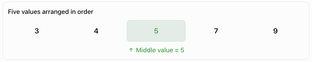
Consider:
7, 3, 9, 5, 4
Arrange in ascending order:
3, 4, 5, 7, 9
There are five values.
The middle value is the third value.
Median = 5
Median Position Formula
For an odd number of values:
Median position = (n + 1)/2
For n = 5:
Median position = (5 + 1)/2 = 3
Therefore, the median is the third value.
Median with an Even Number of Values
When a dataset contains an even number of values, there are two middle values.
The median is the mean of these two values.
Worked Example
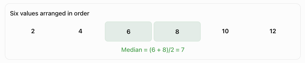
Consider:
4, 8, 2, 10, 6, 12
Arrange in ascending order:
2, 4, 6, 8, 10, 12
There are six values.
The middle values are 6 and 8.
Median = (6 + 8)/2
Median = 7
Important Observation
The median does not have to appear in the original dataset.
In this example, 7 is the median even though no value equals 7.
Why Ordering Matters
Consider:
12, 4, 8, 2, 10
A student might incorrectly select 8 because it appears in the middle of the written list.
However, the values must first be arranged in order:
2, 4, 8, 10, 12
In this particular case, the median is still 8, but this is a coincidence.
Consider instead:
12, 4, 2, 10, 8
The middle value in the original list is 2.
After sorting:
2, 4, 8, 10, 12
the median is 8.
Always arrange numerical data in order before finding the median.
The Mode
The mode is the value that occurs most frequently in a dataset.
The mode is determined by counting how many times each value appears.
Worked Example
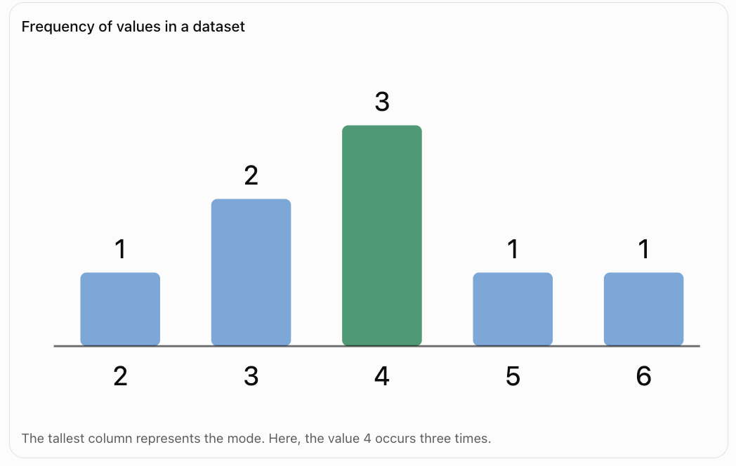
Consider:
2, 4, 3, 4, 5, 4, 6, 3
Count the frequencies:
|
Value |
Frequency |
|---|---|
|
2 |
1 |
|
3 |
2 |
|
4 |
3 |
|
5 |
1 |
|
6 |
1 |
The value 4 appears most often.
Mode = 4
Interpretation
The most common value is 4.
The mode is particularly useful when we want to identify the most frequently occurring result.
Understanding the Mode Visually
Datasets with More Than One Mode
Some datasets contain two or more values that share the highest frequency.
Bimodal Dataset
Consider:
2, 2, 3, 4, 4, 5
Both 2 and 4 appear twice.
All other values appear once.
The dataset has two modes:
Modes = 2 and 4
This is called a bimodal dataset.
Multimodal Dataset
Consider:
1, 1, 2, 2, 3, 3, 4
The values 1, 2, and 3 each appear twice.
Therefore, the dataset has three modes.
A dataset with several modes is called multimodal.
No Mode
Consider:
3, 5, 7, 9, 11
Each value appears once.
Under the usual school convention, this dataset has no mode because no value occurs more frequently than the others.
Mode with Categorical Data
Unlike the mean and median, the mode can be used with non-numerical categories.
For example, students are asked to identify their favourite fruit.
Results:
Apple, Banana, Apple, Orange, Banana, Apple, Mango
The most frequent response is Apple.
Mode = Apple
It would not make sense to calculate the mean of these categories.
The median is also not meaningful because fruit categories do not have a natural numerical order.
The mode is therefore the most appropriate measure of centre for this dataset.

Comparing Mean, Median, and Mode
Although all three measures describe the centre of data, they do so differently.
|
Measure |
How it is calculated |
Main advantage |
Main limitation |
|---|---|---|---|
|
Mean |
Sum ÷ number of values |
Uses every numerical value |
Sensitive to extreme values |
|
Median |
Middle value of ordered data |
Resistant to extreme values |
Does not use the size of every value |
|
Mode |
Most frequent value |
Works with categories |
May be absent or have multiple values |
Worked Example
Consider:
3, 4, 4, 5, 9
Mean:
(3 + 4 + 4 + 5 + 9)/5 = 25/5
Mean = 5
Median:
The middle value is 4.
Median = 4
Mode:
The most frequent value is 4.
Mode = 4
Interpretation
The mean is larger than the median and mode because the high value of 9 increases the average.
The Effect of Outliers
An outlier is a value that is unusually high or low compared with the other values.
Outliers can have a significant effect on the mean.
Example: Household Incomes
Consider five annual household incomes:
$40,000, $45,000, $48,000, $50,000, $52,000
Mean:
= $235,000/5
Mean = $47,000
Median:
Median = $48,000
Now suppose a sixth household with an income of $500,000 is included.
New dataset:
$40,000, $45,000, $48,000, $50,000, $52,000, $500,000
New mean:
= $735,000/6
Mean = $122,500
New median:
= ($48,000 + $50,000)/2
Median = $49,000
Comparison
Mean before
$47,000
Mean after
$122,500
Large increase
Median before
$48,000
Median after
$49,000
Small increase
What Does This Show?
The mean increases dramatically because of the unusually high income.
The median changes only slightly.
For this dataset, the median provides a better description of a typical household income.
This is one reason median income is commonly used in economic and social statistics.
Measures of Centre and Data Distribution
The shape of a dataset can help us decide which measure of centre is most useful.
Symmetrical Distributions
A symmetrical distribution has approximately the same shape on both sides of its centre.
For a perfectly symmetric, unimodal distribution, the mean, median, and mode often coincide.

Right-Skewed Distributions
A right-skewed distribution has a longer tail toward larger values.
High values tend to pull the mean to the right.
In a typical unimodal right-skewed distribution:
Mode < Median < Mean
This ordering is common but not a universal mathematical rule.

Left-Skewed Distributions
A left-skewed distribution has a longer tail toward smaller values.
Low values tend to pull the mean to the left.
In a typical unimodal left-skewed distribution:
Mean < Median < Mode
Again, this is a common pattern rather than a guarantee for every dataset.

Choosing the Most Appropriate Measure
The best measure depends on the type of data and the purpose of the investigation.
When to Use the Mean
The mean is usually appropriate when:
-
Data is numerical.
-
All values should contribute to the calculation.
-
There are no unusually influential outliers.
-
The distribution is reasonably symmetrical.
-
Further calculations require an arithmetic average.
Example: Average temperature measured during an experiment.
When to Use the Median
The median is usually appropriate when:
-
The dataset contains extreme values.
-
The distribution is strongly skewed.
-
A typical middle value is needed.
-
Data can be placed in a meaningful order.
Example: Typical household income or house price.
When to Use the Mode
The mode is usually appropriate when:
-
The most common value is important.
-
Data is categorical.
-
We want to identify the most popular option.
-
Repeated values are meaningful.
Example: Most popular shoe size in a shop.
Practical Application: Choosing Shoe Sizes
A shoe shop records the sizes of shoes sold during one day.
|
Shoe size |
Number sold |
|---|---|
|
6 |
3 |
|
7 |
5 |
|
8 |
12 |
|
9 |
9 |
|
10 |
4 |
|
11 |
2 |
The shop wants to decide which size to stock most heavily.
The most appropriate measure is the mode.
Mode = Size 8
Size 8 was sold 12 times, more than any other size.
Although the mean shoe size could be calculated, it would not directly identify the most popular size.
Practical Application: Comparing Two Classes
Two classes complete the same assessment.
Assessment scores
Class A
6, 7, 7, 8, 8, 9, 10
Mean = 7.86
Median = 8
Modes = 7 and 8
Class B
3, 5, 7, 8, 9, 10, 10
Mean = 7.43
Median = 8
Mode = 10
Interpretation
Both classes have the same median score of 8.
Class A has a slightly higher mean.
Class B has the highest possible mode of 10, but it also has several low scores.
This demonstrates why relying on only one measure of centre can be misleading.
The mean, median, and mode provide different information about the same dataset.
Real-World Application: Scientific Measurements
A scientist measures the height of six plants after four weeks.
The heights are:
12, 14, 13, 15, 14, 16 cm
Mean
Sum = 12 + 14 + 13 + 15 + 14 + 16 = 84
Mean = 84/6
Mean = 14 cm
Median
Arrange the data:
12, 13, 14, 14, 15, 16
The middle values are 14 and 14.
Median = 14 cm
Mode
The value 14 appears twice.
Mode = 14 cm
Interpretation
All three measures are equal.
This suggests that 14 cm is a reasonable central value for the measurements.
However, measures of centre alone do not describe the variation in plant heights. Measures such as range and standard deviation would provide additional information.

Comparing Datasets with the Same Mean
Two datasets can have the same mean but very different distributions.
Consider:
Dataset A:
4, 5, 6, 7, 8
Dataset B:
0, 0, 5, 10, 15
Dataset A
Mean = 30/5 = 6
Median = 6
Mode = none
Dataset B
Mean = 30/5 = 6
Median = 5
Mode = 0
Both datasets have the same mean, but the values are distributed differently.
Dataset B contains much greater variation.
This demonstrates why a measure of centre should often be considered alongside a measure of spread.
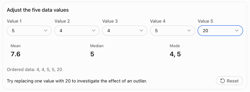
Interactive Practice: Calculate the Measures of Centre
Change the values in the dataset and observe how the mean, median, and mode respond.
Common Mistakes
Forgetting to divide when calculating the mean
The mean is the sum of the values divided by the number of values.
Dividing by the wrong number
Count every observation, including repeated values.
Failing to order the data before finding the median
The median depends on numerical order.
Selecting only one middle value for an even-sized dataset
When there are two middle values, calculate their mean.
Confusing the mode with the largest value
The mode is the most frequent value, not necessarily the greatest value.
Assuming every dataset has exactly one mode
A dataset can have no mode, one mode, or several modes.
Assuming the mean must appear in the dataset
The mean can be a decimal even when all values are whole numbers.
Ignoring outliers
Extreme values can substantially change the mean.
Using the mean for categorical data
Categories such as favourite colours cannot meaningfully be averaged.
Assuming the mean, median, and mode always agree
They often differ, especially in skewed distributions.
Reporting a measure without context
Always include appropriate units and explain what the value represents.
Key Terms
-
Data: Information collected for analysis.
-
Dataset: Collection of observations or values.
-
Observation: Individual value recorded in a dataset.
-
Measure of Centre: Statistic used to describe a typical or central value.
-
Central Tendency: Tendency of data to cluster around a central value.
-
Mean: Sum of numerical values divided by their number.
-
Arithmetic Mean: Another name for the ordinary mean.
-
Median: Middle value of an ordered dataset.
-
Mode: Most frequently occurring value.
-
Frequency: Number of times a value occurs.
-
Frequency Table: Table showing values and their frequencies.
-
Bimodal: Having two modes.
-
Multimodal: Having more than one mode.
-
Outlier: Value unusually far from the other observations.
-
Distribution: Pattern showing how data values are spread.
-
Symmetrical Distribution: Distribution with approximately matching sides.
-
Right-Skewed Distribution: Distribution with a longer tail toward larger values.
-
Left-Skewed Distribution: Distribution with a longer tail toward smaller values.
-
Categorical Data: Data describing categories or labels.
-
Numerical Data: Data represented by numbers with quantitative meaning.
-
Measure of Spread: Statistic describing variability in a dataset.
-
Representative Value: Value used to summarise a dataset.
Key Takeaways
-
Measures of centre describe typical or central values in a dataset.
-
The three main measures are mean, median, and mode.
-
The mean is calculated by dividing the sum of values by the number of values.
-
The median is the middle value after sorting the dataset.
-
For an even number of values, the median is the mean of the two middle values.
-
The mode is the most frequently occurring value.
-
A dataset may have multiple modes or no mode.
-
The mean is sensitive to unusually large or small values.
-
The median is resistant to outliers.
-
The mode can be used with categorical data.
-
Symmetrical datasets often have similar measures of centre.
-
Skewed datasets may have noticeably different means, medians, and modes.
-
The most appropriate measure depends on the data type and purpose.
-
Measures of centre should often be interpreted alongside measures of spread.
Check Your Understanding
Calculate the mean, median, and mode where appropriate.
-
2, 4, 6, 8, 10
-
3, 3, 5, 7, 7, 7
-
10, 15, 20, 25
-
4, 6, 6, 8, 10, 12
-
1, 2, 3, 4, 100
-
5, 5, 6, 6, 7, 8
-
12, 14, 16, 18, 20
-
2, 2, 3, 4, 4, 5, 5
-
7, 9, 11, 13, 15, 17
-
1.5, 2.0, 2.5, 3.0, 3.5
Answer the following questions.
-
Why must data be ordered before finding the median?
-
Which measure of centre is most affected by outliers?
-
Which measure is most appropriate for favourite colours?
-
Why is the median often preferred for household income?
-
Can a dataset have more than one mode?
Answers
|
Question |
Mean |
Median |
Mode |
|---|---|---|---|
|
1 |
6 |
6 |
None |
|
2 |
5.33 |
6 |
7 |
|
3 |
17.5 |
17.5 |
None |
|
4 |
7.67 |
7 |
6 |
|
5 |
22 |
3 |
None |
|
6 |
6.17 |
6 |
5 and 6 |
|
7 |
16 |
16 |
None |
|
8 |
3.57 |
4 |
2, 4 and 5 |
|
9 |
12 |
12 |
None |
|
10 |
2.5 |
2.5 |
None |
-
The median is determined by position in an ordered dataset.
-
The mean.
-
The mode.
-
It is less affected by extreme income values.
-
Yes. A dataset can be bimodal or multimodal.
Extended Challenge
Calculating Measures of Centre
-
Calculate the mean, median, and mode of: 12, 15, 15, 18, 20, 20, 20, 25.
-
Calculate the mean and median of: 3, 7, 8, 9, 12, 15.
-
Find the missing value if the mean of 4, 6, 8, x, 12 is 8.
-
Five numbers have a mean of 14. What is their total?
-
Six values have a total of 90. What is their mean?
Comparing Datasets
-
Dataset A: 5, 6, 7, 8, 9. Dataset B: 1, 3, 7, 11, 13. Compare their means and medians.
-
Create two different datasets with the same mean but different medians.
-
Create a dataset with exactly two modes.
-
Create a dataset with no mode.
-
Explain how adding a very large value changes the mean and median of a dataset.
Selecting Appropriate Measures
-
A school wants to identify the most common lunch choice. Which measure should be used?
-
A real estate company wants to describe typical house prices in an area containing several luxury homes. Which measure is likely most appropriate?
-
A scientist records 100 measurements from a stable instrument. Which measure might best represent the overall average?
-
A clothing store wants to determine which shirt size to order most frequently. Which measure should be used?
-
A researcher compares the incomes of two communities. Explain why reporting both mean and median may be useful.
Final Challenge: Statistical Investigation
A school records the time, in minutes, taken by 15 students to complete a mathematics activity.
The times are:
12, 15, 14, 18, 16, 15, 13, 17, 14, 15, 20, 16, 14, 19, 42
Complete the investigation.
-
Arrange the data in ascending order.
-
Calculate the mean completion time.
-
Determine the median completion time.
-
Identify the mode.
-
Construct a frequency table.
-
Identify any value that appears unusually high or low.
-
Explain how the unusually high value affects the mean.
-
Recalculate the mean after excluding the value 42, clearly stating that you have changed the dataset.
-
Compare the two means.
-
Determine whether the median changes when 42 is excluded.
-
Decide which measure of centre best represents a typical student's completion time.
-
Justify your choice using evidence.
-
Explain why reporting only the mean could be misleading.
-
Describe one possible reason for the unusually high completion time.
-
Write a short conclusion explaining what the dataset reveals about student performance.
Further Investigation
Collect a dataset of at least 20 values from a real situation, such as daily temperatures, travel times, test scores, or plant heights.
Calculate the mean, median, and mode. Construct an appropriate graph and investigate whether the distribution is symmetrical or skewed.
Explain which measure of centre provides the most meaningful summary and why.
2. Measures of Spread
Learning outcomes
- I can calculate the range.
- I can calculate the interquartile range.
- I can calculate the variance.
- I can calculate the standard deviation.
- I can interpret measures of variability.
Measures of Spread
Introduction
Measures of centre, such as the mean, median, and mode, help us describe a typical value in a dataset. However, knowing the centre does not tell us how widely the values are distributed.
Consider two groups of students who complete the same mathematics assessment.
Class A: 6, 7, 8, 9, 10
Class B: 2, 5, 8, 11, 14
Both classes have a mean score of 8.
However, the scores in Class A are clustered closely around the mean, while the scores in Class B are much more widely distributed.
This difference is described using measures of spread, also called measures of dispersion or variability.
The four measures we will investigate are:
-
Range: Difference between the highest and lowest values.
-
Interquartile range (IQR): Spread of the middle 50% of values.
-
Variance: Average squared deviation from the mean, with different formulas for populations and samples.
-
Standard deviation: Measure of how far values typically vary around the mean.
These measures are used in science, economics, education, manufacturing, medicine, and many other fields.


What Is Variability?
Variability describes how much the values in a dataset differ from one another.
A dataset with low variability has values that are relatively close together.
A dataset with high variability has values that are more widely dispersed.
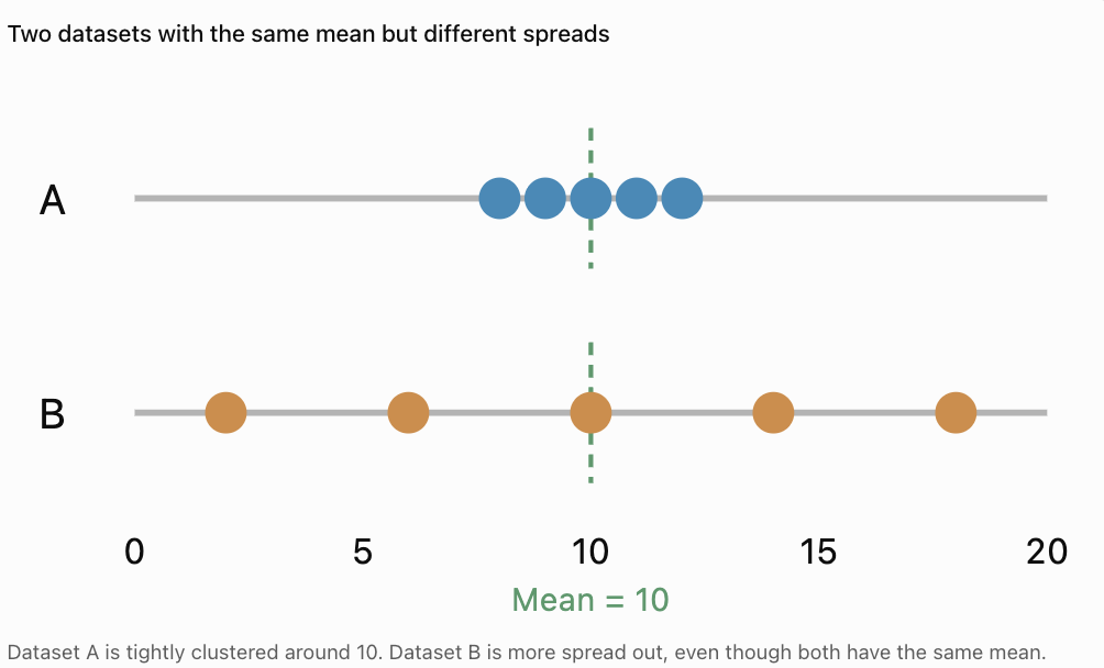
Example
Consider:
Dataset A: 8, 9, 10, 11, 12
Dataset B: 2, 6, 10, 14, 18
Both datasets have:
Mean = 10
However, Dataset B has much greater variability.
Why Is Variability Important?
Variability helps us understand:
-
Whether results are consistent.
-
Whether measurements are reliable.
-
How much individuals differ.
-
Whether a typical value represents the whole dataset well.
-
Whether unusual values may be present.
For example, two machines might produce objects with the same average mass, but one machine may produce much more consistent results.
The Range
The range is the simplest measure of spread.
It is the difference between the largest and smallest values in a dataset.
Range = Maximum value − Minimum value
Worked Example: Test Scores
Consider:
12, 15, 18, 20, 25
The maximum value is 25.
The minimum value is 12.
Range = 25 − 12
Range = 13
Interpretation
The highest score is 13 points greater than the lowest score.
The range tells us the total width of the dataset.
Finding the Range with Negative Numbers
The range can also be calculated for datasets containing negative values.
Worked Example: Temperatures
A weather station records these temperatures:
−4, −2, 1, 3, 6°C
Maximum = 6°C
Minimum = −4°C
Range = 6 − (−4)
Range = 6 + 4
Range = 10°C
Important Reminder
Subtracting a negative number is equivalent to adding its positive value.
Strengths and Limitations of the Range
Advantages
-
Very easy to calculate.
-
Quickly describes the total spread.
-
Useful for comparing minimum and maximum measurements.
-
Can be calculated for small datasets.
Limitations
-
Uses only two values.
-
Does not describe the distribution of the middle values.
-
Can be strongly affected by outliers.
-
May change dramatically when a single extreme value is added.
Example
Dataset A:
5, 6, 7, 8, 9
Range = 9 − 5 = 4
Dataset B:
5, 6, 7, 8, 100
Range = 100 − 5 = 95
Replacing one value with an extreme observation increases the range dramatically.
The range is useful, but it should not always be used alone.
Quartiles
Quartiles divide an ordered dataset into four parts.
The three quartiles are:
-
First quartile (Q1): Lower quartile, associated with the 25th percentile.
-
Second quartile (Q2): Median, associated with the 50th percentile.
-
Third quartile (Q3): Upper quartile, associated with the 75th percentile.
Quartiles help us understand where values are concentrated.
Example
Consider the ordered dataset:
2, 4, 5, 7, 8, 10, 12, 14, 16
The median is the fifth value:
Q2 = 8
Using the median-of-halves method, exclude the overall median and divide the remaining values into two halves.
Lower half:
2, 4, 5, 7
Upper half:
10, 12, 14, 16
Find the median of each half.
Q1 = (4 + 5)/2 = 4.5
Q3 = (12 + 14)/2 = 13
Therefore:
Q1 = 4.5
Q2 = 8
Q3 = 13
Important Note About Quartile Methods
Different textbooks, calculators, and statistical software may calculate quartiles using slightly different conventions.
In these notes, we use the median-of-halves method:
-
For an odd-sized dataset, exclude the overall median when forming the halves.
-
For an even-sized dataset, divide the values into equal lower and upper halves.
-
Find the median of each half.
Always use the method required by your course or assessment.
The Interquartile Range
The interquartile range (IQR) measures the spread of the middle 50% of a dataset.
It is calculated by subtracting the first quartile from the third quartile.
IQR = Q3 − Q1
Worked Example
Using the previous dataset:
2, 4, 5, 7, 8, 10, 12, 14, 16
We found:
Q1 = 4.5
Q3 = 13
Therefore:
IQR = 13 − 4.5
IQR = 8.5
Interpretation
The middle half of the dataset extends across an interval with width 8.5.
Unlike the range, the IQR focuses on the central portion of the data.
Finding the IQR with an Even Number of Values
Worked Example
Consider:
3, 5, 7, 8, 10, 12, 14, 18
There are eight values.
Divide the ordered dataset into two equal halves.
Lower half:
3, 5, 7, 8
Upper half:
10, 12, 14, 18
Calculate Q1:
Q1 = (5 + 7)/2 = 6
Calculate Q3:
Q3 = (12 + 14)/2 = 13
Therefore:
IQR = 13 − 6
IQR = 7
Understanding the IQR with Box Plots
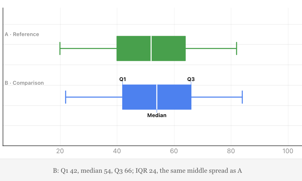
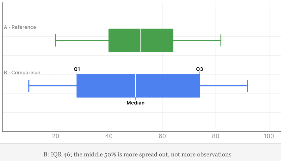
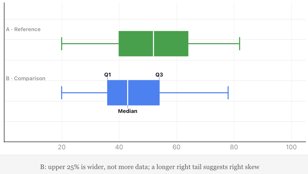
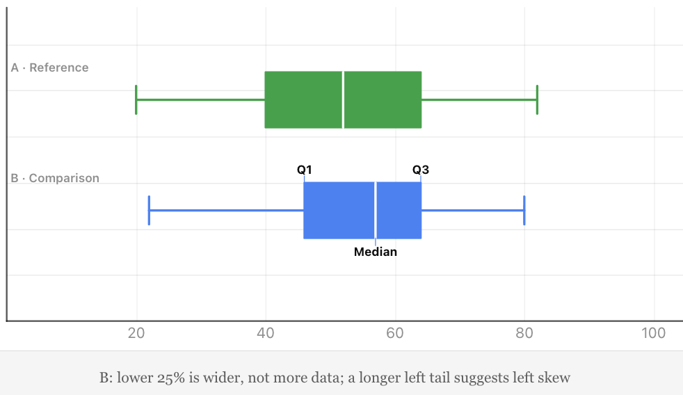
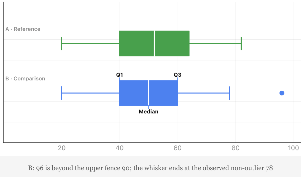
A box plot displays the distribution of numerical data using quartiles, the median, and whiskers.
The box extends from Q1 to Q3.
Its width represents the interquartile range.
A line inside the box represents the median.
In a modified box plot, whiskers usually extend to the most extreme observed values that are not classified as outliers.
Interpreting a Box Plot
A wide box indicates that the middle 50% of values has a large spread.
A narrow box indicates that the middle 50% is more closely clustered.
Box plots are particularly useful for comparing two or more datasets.
Why Is the IQR Useful?
The IQR is resistant to extreme values because it focuses on the middle half of the dataset.
For this reason, it is often preferred when data is skewed or contains outliers.
Identifying Possible Outliers Using the IQR
The IQR can help identify unusually high or low values.
A common method is the 1.5 × IQR rule.
Calculate:
Lower fence = Q1 − 1.5 × IQR
Upper fence = Q3 + 1.5 × IQR
Values outside these fences are flagged as potential outliers.
Worked Example
Consider:
2, 3, 4, 5, 6, 7, 8, 9, 30
Using the median-of-halves method:
Q1 = (3 + 4)/2 = 3.5
Q3 = (8 + 9)/2 = 8.5
IQR = 8.5 − 3.5 = 5
Calculate the fences.
Lower fence:
3.5 − 1.5(5) = −4
Upper fence:
8.5 + 1.5(5) = 16
Therefore, values below −4 or above 16 are potential outliers.
Since:
30 > 16
30 is a potential outlier.
Important Interpretation
A potential outlier is not necessarily an error.
It may represent a genuine but unusual observation.
Investigators should examine possible outliers before deciding whether to exclude them.
Variance
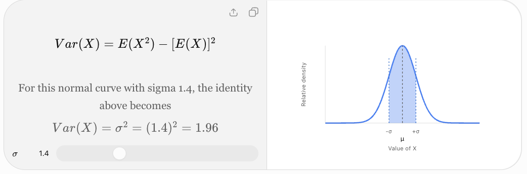
The variance measures how widely numerical values are distributed around their mean.
It is based on the squared differences between each value and the mean.
These differences are called deviations.
Why Square the Deviations?
Consider values above and below the mean.
Some deviations are positive, while others are negative.
If we simply add all deviations from the mean, the total is zero.
Squaring the deviations:
-
Makes every contribution nonnegative.
-
Prevents positive and negative deviations from cancelling.
-
Gives greater weight to values far from the mean.
Variance is therefore a useful mathematical measure of variability.
Population Variance and Sample Variance
There are two commonly used variance formulas.
Population Variance
A population contains every member or observation in the group being studied.
Population variance is:
σ² = Σ(x − μ)²/N
Where:
-
σ² = population variance
-
x = individual value
-
μ = population mean
-
N = number of values in the population
-
Σ = sum of all values
Sample Variance
A sample is a subset selected from a larger population.
Sample variance is:
s² = Σ(x − x̄)²/(n − 1)
Where:
-
s² = sample variance
-
x = individual value
-
x̄ = sample mean
-
n = number of sample observations
Why Divide by n − 1?
When we calculate variance from a sample, dividing by n − 1 rather than n corrects for the tendency of the sample's squared deviations to underestimate the population variance.
This is called Bessel's correction.
For a sample of independent observations from a population with finite variance, the n − 1 formula gives an unbiased estimator of population variance.
Which Formula Should You Use?
Use the population formula when your dataset represents the entire population of interest.
Use the sample formula when your data is a sample and you want to estimate the variability of the larger population.
Calculating Population Variance Step by Step
Worked Example
Consider the dataset:
2, 4, 6, 8, 10
Treat these five values as the entire population.
Step 1: Calculate the Mean
Mean = (2 + 4 + 6 + 8 + 10)/5
Mean = 30/5
μ = 6
Step 2: Find Each Deviation
Subtract the mean from each value.
|
x |
x − μ |
(x − μ)² |
|---|---|---|
|
2 |
−4 |
16 |
|
4 |
−2 |
4 |
|
6 |
0 |
0 |
|
8 |
2 |
4 |
|
10 |
4 |
16 |
|
Total |
0 |
40 |
Step 3: Add the Squared Deviations
Σ(x − μ)² = 40
Step 4: Divide by N
σ² = 40/5
Population variance = 8
Interpretation
The variance describes the average squared distance from the mean.
Because the original values have no specified units, the variance is expressed in squared data units.
If these were measurements in centimetres, the variance would be 8 cm².
Understanding Squared Deviations
The further a value is from the mean, the larger its squared deviation becomes.
For example:
-
A deviation of 1 contributes 1 to the squared total.
-
A deviation of 2 contributes 4.
-
A deviation of 3 contributes 9.
-
A deviation of 5 contributes 25.
This means extreme values can have a substantial effect on variance.
Important Observation
Variance is always greater than or equal to zero.
It equals zero only when every value in the dataset is identical.
Calculating Sample Variance
Worked Example
Suppose the values:
2, 4, 6, 8, 10
are a sample from a larger population.
The mean is:
x̄ = 6
The sum of squared deviations is:
Σ(x − x̄)² = 40
However, because the dataset is a sample:
s² = 40/(5 − 1)
s² = 40/4
Sample variance = 10
Comparison
For the same five observations:
-
Population variance = 8
-
Sample variance = 10
The sample variance is larger because we divide by n − 1 instead of n.
This distinction is essential when interpreting statistical results.
Standard Deviation
The standard deviation measures the spread of data around the mean.
It is calculated by taking the square root of the variance.
Standard deviation is especially useful because it is expressed in the same units as the original data.
Population Standard Deviation
σ = √[Σ(x − μ)²/N]
Sample Standard Deviation
s = √[Σ(x − x̄)²/(n − 1)]
Relationship Between Variance and Standard Deviation
Standard deviation = √Variance
Variance = (Standard deviation)²
Calculating Standard Deviation Step by Step
Using the dataset:
2, 4, 6, 8, 10
we previously found:
Population variance = 8
Therefore:
σ = √8
Population standard deviation ≈ 2.83
If the data represents a sample:
Sample variance = 10
Therefore:
s = √10
Sample standard deviation ≈ 3.16
Interpretation
The population standard deviation of approximately 2.83 indicates the scale of variation around the mean of 6.
Standard deviation is often described informally as a typical distance from the mean, although it is specifically the root mean square of the deviations rather than the ordinary average absolute distance.
Understanding Standard Deviation Visually
Standard deviation helps us compare how tightly or widely values cluster around their mean.
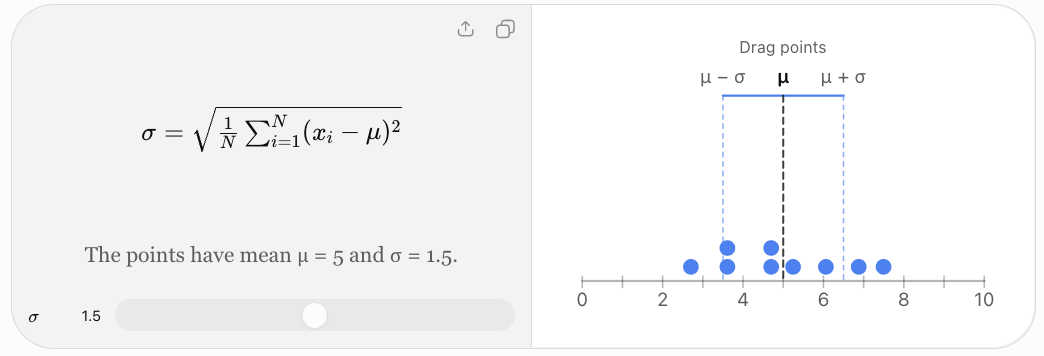
Small Standard Deviation
A small standard deviation indicates that values are relatively close to the mean.
Large Standard Deviation
A large standard deviation indicates that values are more widely spread around the mean.
Zero Standard Deviation
If all values are identical, the standard deviation is zero.
For example:
5, 5, 5, 5, 5
Mean = 5
Every deviation is zero.
Therefore:
Variance = 0
Standard deviation = 0
Comparing Two Datasets Using Standard Deviation
Consider:
Dataset A:
8, 9, 10, 11, 12
Dataset B:
2, 6, 10, 14, 18
Both have:
Mean = 10
Dataset A
Deviations:
−2, −1, 0, 1, 2
Squared deviations:
4, 1, 0, 1, 4
Sum = 10
Population variance:
σ² = 10/5 = 2
Standard deviation:
σ ≈ 1.41
Dataset B
Deviations:
−8, −4, 0, 4, 8
Squared deviations:
64, 16, 0, 16, 64
Sum = 160
Population variance:
σ² = 160/5 = 32
Standard deviation:
σ ≈ 5.66
Comparison
|
Measure |
Dataset A |
Dataset B |
|---|---|---|
|
Mean |
10 |
10 |
|
Range |
4 |
16 |
|
Population variance |
2 |
32 |
|
Population standard deviation |
1.41 |
5.66 |
Dataset B has much greater variability, despite having the same mean.
Standard Deviation and the Normal Distribution
A normal distribution is a symmetrical, bell-shaped distribution.
For data that follows a normal distribution approximately:
-
About 68% of observations lie within 1 standard deviation of the mean.
-
About 95% lie within 2 standard deviations.
-
About 99.7% lie within 3 standard deviations.
This is known as the 68–95–99.7 rule, or empirical rule.

Worked Example
Suppose examination scores are approximately normally distributed with:
Mean = 70
Standard deviation = 10
Then approximately:
-
68% of scores fall between 60 and 80.
-
95% fall between 50 and 90.
-
99.7% fall between 40 and 100.
These are approximate proportions under the assumed normal model, not guarantees for every dataset.
Important Limitation
The empirical rule should not be applied automatically to strongly skewed or irregular distributions.
Comparing Range, IQR, Variance, and Standard Deviation
|
Measure |
Calculation |
Units |
Sensitivity to outliers |
|---|---|---|---|
|
Range |
Maximum − minimum |
Original units |
Very high |
|
IQR |
Q3 − Q1 |
Original units |
Relatively low |
|
Population variance |
Mean squared deviation |
Squared units |
High |
|
Population standard deviation |
Square root of variance |
Original units |
High |
When Is Each Measure Useful?
Range: When the total difference between the smallest and largest values is important.
IQR: When describing the spread of the middle half of a dataset, particularly if the data is skewed.
Variance: When performing mathematical and statistical calculations involving squared deviations.
Standard deviation: When describing variability around the mean using the original units.
Measures of Centre and Spread Together
A measure of centre describes a typical value.
A measure of spread describes how much values vary around that typical value.
Both are important.
For example, two schools may have the same mean test score but different standard deviations.
A school with a smaller standard deviation has scores that are more tightly clustered around its mean.
A school with a larger standard deviation has greater variation in student performance.
Useful Reporting Combinations
For approximately symmetrical numerical data:
Mean and standard deviation
For skewed numerical data or data with outliers:
Median and interquartile range
These are common reporting conventions, not absolute rules.
Real-World Application: Manufacturing Quality Control
A factory produces metal rods intended to have a length of 50 cm.
Two machines produce the following samples.
Machine A:
49.9, 50.0, 50.1, 50.0, 50.0
Machine B:
49.5, 50.4, 50.0, 50.6, 49.5
Both machines have a mean length of 50.0 cm.
However, Machine A produces rods with much less variation.
Machine A
Population variance:
σ² = (0.01 + 0 + 0.01 + 0 + 0)/5
= 0.004 cm²
Standard deviation:
σ ≈ 0.063 cm
Machine B
Squared deviations:
0.25, 0.16, 0, 0.36, 0.25
Sum = 1.02
Population variance:
σ² = 1.02/5 = 0.204 cm²
Standard deviation:
σ ≈ 0.452 cm
Interpretation
Machine A is more consistent.
Even though both machines have the same mean, Machine B produces rods with a much greater spread of lengths.

Real-World Application: Comparing Student Performance
Two students complete five assessments.
Student A:
78, 80, 82, 79, 81
Student B:
60, 70, 80, 90, 100
Both have:
Mean = 80
Student A
Squared deviations from 80:
4, 0, 4, 1, 1
Sum = 10
Population variance = 10/5 = 2
Population standard deviation:
σ ≈ 1.41
Student B
Squared deviations:
400, 100, 0, 100, 400
Sum = 1000
Population variance = 1000/5 = 200
Population standard deviation:
σ ≈ 14.14
Interpretation
Student A demonstrates much more consistent performance.
Student B has greater variation, including both much lower and much higher scores.
Standard deviation reveals this difference even though the mean scores are identical.
Real-World Application: Scientific Experiments
Suppose two groups of plants are grown under different conditions.
The mean plant height in both groups is 15 cm.
However:
Group A has a standard deviation of 1 cm.
Group B has a standard deviation of 4 cm.
Interpretation
Group A has more consistent plant heights.
Group B has greater variation.
This could suggest differences in environmental conditions, genetics, measurement quality, or other factors.
However, the standard deviation alone cannot establish the cause of the variability.
Scientists must consider the experimental design and other evidence.

Using Technology to Calculate Measures of Spread
Calculators and spreadsheets can calculate variance and standard deviation efficiently.
For example, in a spreadsheet with values in cells A1 through A10:
|
Calculation |
Spreadsheet formula |
|---|---|
|
Range |
|
|
Population variance |
|
|
Sample variance |
|
|
Population standard deviation |
|
|
Sample standard deviation |
|
For quartiles, spreadsheet functions such as QUARTILE.INC and QUARTILE.EXC are available, but their results may differ from the median-of-halves convention used in these notes.
Important Reminder
Technology can perform calculations quickly, but students should understand what each measure represents and how it is calculated.
Common Mistakes
Confusing range with interquartile range
The range uses the maximum and minimum values. The IQR uses Q3 and Q1.
Forgetting to order data before finding quartiles
Quartiles depend on the positions of values in an ordered dataset.
Using inconsistent quartile methods
Different methods can produce different results, particularly for small datasets.
Subtracting quartiles in the wrong order
IQR = Q3 − Q1, not Q1 − Q3.
Confusing variance and standard deviation
Standard deviation is the square root of variance.
Forgetting to square deviations
Variance requires squared differences from the mean.
Forgetting to take the square root
Calculating variance is not the final step when standard deviation is required.
Using the wrong denominator
Population variance uses N. Sample variance uses n − 1.
Rounding too early
Keep sufficient decimal places during calculations and round the final answer.
Ignoring units
Variance uses squared units, while standard deviation uses the original units.
Assuming a large standard deviation always indicates poor results
A large standard deviation indicates variability, not necessarily poor quality or performance.
Ignoring outliers
Extreme observations can strongly influence range, variance, and standard deviation.
Applying the empirical rule to every distribution
The 68–95–99.7 rule applies to approximately normal distributions.
Key Terms
-
Variability: Degree to which values differ within a dataset.
-
Dispersion: Another term for the spread of data.
-
Range: Difference between the maximum and minimum values.
-
Quartile: Value used to divide ordered data into four parts.
-
First Quartile (Q1): Lower quartile.
-
Second Quartile (Q2): Median.
-
Third Quartile (Q3): Upper quartile.
-
Interquartile Range (IQR): Difference between Q3 and Q1.
-
Five-Number Summary: Minimum, Q1, median, Q3, and maximum.
-
Box Plot: Graph displaying quartiles, median, and whiskers.
-
Outlier: Observation unusually far from other values.
-
Outlier Fence: Boundary used to identify potential outliers.
-
Variance: Measure based on squared deviations from the mean.
-
Standard Deviation: Square root of variance.
-
Deviation: Difference between a value and the mean.
-
Squared Deviation: Square of a deviation.
-
Population: Entire group of interest.
-
Sample: Subset of a population.
-
Population Variance: Variance calculated using the population mean and population size.
-
Sample Variance: Variance estimate calculated using the sample mean and n − 1.
-
Bessel's Correction: Use of n − 1 when calculating sample variance.
-
Normal Distribution: Symmetrical bell-shaped probability distribution.
-
Empirical Rule: Approximate 68–95–99.7 pattern for normal distributions.
-
Consistency: Degree to which measurements or results remain similar.
-
Skewness: Asymmetry in the distribution of data.
Key Takeaways
-
Measures of spread describe variability in a dataset.
-
The range is the difference between the largest and smallest values.
-
Quartiles divide ordered data into four parts.
-
The interquartile range describes the spread of the middle 50% of observations.
-
The IQR is relatively resistant to extreme values.
-
Variance is based on squared deviations from the mean.
-
Population variance uses N in the denominator.
-
Sample variance uses n − 1 in the denominator.
-
Standard deviation is the square root of variance.
-
Standard deviation uses the same units as the original data.
-
A small standard deviation indicates relatively consistent values.
-
A large standard deviation indicates greater variability.
-
Extreme values can strongly influence variance and standard deviation.
-
Mean and standard deviation are often reported together for approximately symmetrical data.
-
Median and IQR are often preferred for skewed data.
-
Measures of centre and spread should be interpreted together.
Check Your Understanding
Range
-
Find the range of 4, 7, 9, 12, 15.
-
Find the range of −5, −2, 3, 7, 10.
-
Find the range of 12, 12, 12, 12.
-
A dataset has a minimum of 8 and maximum of 37. Find the range.
Interquartile Range
Use the median-of-halves method.
-
Find the IQR of 2, 4, 6, 8, 10, 12, 14.
-
Find the IQR of 3, 5, 7, 9, 11, 13, 15, 17.
-
A dataset has Q1 = 12 and Q3 = 28. Find the IQR.
-
Explain why the IQR is less sensitive to outliers than the range.
Variance
Treat the following datasets as populations unless stated otherwise.
-
Find the population variance of 2, 4, 6.
-
Find the population variance of 5, 5, 5, 5.
-
Find the population variance of 1, 3, 5, 7.
-
A sample has values 2, 4, 6. Calculate the sample variance.
Standard Deviation
-
Find the population standard deviation of 2, 4, 6.
-
Find the population standard deviation of 5, 5, 5, 5.
-
A population has variance 25. Find its standard deviation.
-
A sample has variance 16. Find its sample standard deviation.
Interpretation
-
Which measure of spread is most strongly affected by a single extreme value: range or IQR?
-
Why is standard deviation easier to interpret than variance in terms of units?
-
Can two datasets have the same mean but different standard deviations?
-
Explain what a standard deviation of zero means.
Answers
|
Question |
Answer |
|---|---|
|
1 |
11 |
|
2 |
15 |
|
3 |
0 |
|
4 |
29 |
|
5 |
8 |
|
6 |
8 |
|
7 |
16 |
|
8 |
The IQR uses the middle half rather than the extreme values |
|
9 |
8/3 ≈ 2.67 |
|
10 |
0 |
|
11 |
5 |
|
12 |
4 |
|
13 |
√(8/3) ≈ 1.63 |
|
14 |
0 |
|
15 |
5 |
|
16 |
4 |
|
17 |
Range |
|
18 |
It uses the original data units |
|
19 |
Yes |
|
20 |
All values are identical |
Extended Challenge
Calculating Range and IQR
-
Find the range and IQR of 4, 6, 8, 10, 12, 14, 16.
-
Find the range and IQR of 2, 3, 5, 7, 9, 12, 15, 20.
-
Find the range and IQR of 10, 10, 12, 14, 15, 18, 20, 25, 30.
-
Construct a dataset with a range of 20 and an IQR of 5.
-
Explain how adding an extreme value might change the range and IQR.
Calculating Variance
-
Find the population variance of 3, 5, 7, 9.
-
Find the sample variance of 3, 5, 7, 9.
-
Find the population variance of 10, 12, 14, 16, 18.
-
Find the sample variance of 4, 6, 8, 10, 12.
-
Explain why sample variance is generally larger than population variance when both formulas are applied to the same nonconstant dataset.
Calculating Standard Deviation
-
Find the population standard deviation of 1, 2, 3, 4, 5.
-
Find the sample standard deviation of 1, 2, 3, 4, 5.
-
Find the population standard deviation of 20, 22, 24, 26, 28.
-
Find the sample standard deviation of 5, 10, 15, 20.
-
Explain why standard deviation cannot be negative.
Interpretation and Comparison
-
Two datasets have the same mean but standard deviations of 2 and 9. Compare their variability.
-
Explain why IQR may be preferred for income data.
-
Explain why standard deviation is useful in manufacturing.
-
Describe a situation where the range is more informative than the standard deviation.
-
Explain why measures of centre and spread should be reported together.
Final Challenge: Comparing Two Scientific Experiments
Two groups of plants are grown under different environmental conditions.
After four weeks, their heights are measured in centimetres.
Group A:
12, 13, 14, 14, 15, 15, 16, 17, 18
Group B:
6, 9, 11, 14, 15, 16, 19, 22, 27
Complete the investigation.
-
Calculate the mean height of each group.
-
Calculate the median height of each group.
-
Determine the range of each group.
-
Find Q1 and Q3 for each group using the median-of-halves method.
-
Calculate the IQR for each group.
-
Construct a five-number summary for each group.
-
Draw comparative box plots.
-
Calculate the population variance for each group, treating each group as the complete set of plants under investigation.
-
Calculate the population standard deviation for each group.
-
Compare the variability of the two groups.
-
Identify which group has more consistent plant heights.
-
Determine whether either group contains potential outliers using the 1.5 × IQR rule.
-
Explain how the range and IQR provide different information.
-
Explain how the standard deviations support your conclusions.
-
Discuss why two groups can have similar means but different spreads.
-
Suggest possible environmental factors that could influence plant growth.
-
Explain why variability is important when interpreting experimental results.
-
Identify one limitation of drawing conclusions from these datasets alone.
-
Recommend which measures of centre and spread should be reported.
-
Write a scientific conclusion comparing the two groups.
Further Investigation: Data Collection
Collect at least 20 numerical observations from a real-world situation.
Possible investigations include:
-
Time taken by students to complete an activity.
-
Daily temperatures over several weeks.
-
Heights of plants grown under similar conditions.
-
Distances travelled to school.
-
Scores on a classroom assessment.
Calculate the range, quartiles, IQR, variance, and standard deviation.
Present your results in a table and construct a suitable graph.
Finally, explain what the measures reveal about the consistency and variability of the data, and discuss whether any observations appear unusual.
3. Percentiles and Standard Scores
Learning outcomes
- I can calculate percentiles.
- I can interpret percentile rankings.
- I can calculate z-scores.
- I can compare observations using standard scores.
- I can interpret standardized data.
Understanding the Mean and Standard Deviation
Before calculating z-scores, we need to understand two statistical measures.
Mean
The mean is the arithmetic average of a dataset.
Mean = Sum of observations / Number of observations
Consider:
4, 6, 8, 10, 12
Mean = (4 + 6 + 8 + 10 + 12)/5
Mean = 40/5
Mean = 8
Standard Deviation
Standard deviation measures how spread out the observations are around the mean.
A small standard deviation indicates that values tend to be close to the mean.
A large standard deviation indicates that values are more widely spread.
For a population:
σ = √[Σ(x − μ)²/N]
where:
-
σ = population standard deviation
-
x = individual observation
-
μ = population mean
-
N = number of observations
For a sample, the corresponding formula uses the sample mean and divides by n − 1 rather than n.
Example
Two classes both have a mean examination score of 70.
Class A has a standard deviation of 5.
Class B has a standard deviation of 15.
Scores in Class A are more closely clustered around 70.
Scores in Class B are more widely spread.
A score of 85 is therefore much more unusual in Class A than in Class B.
Calculating z-Scores
The formula for a z-score is:
z = (x − μ)/σ
where:
-
z = standard score
-
x = observation
-
μ = population mean
-
σ = population standard deviation
If using a sample mean and sample standard deviation, the analogous calculation is:
z = (x − x̄)/s
The numerator measures how far the observation is from the mean.
The denominator expresses that distance in standard deviation units.
Worked Example: Examination Score
A mathematics examination has:
Mean = 70
Standard deviation = 10
A student scores 85.
Find the z-score.
Step 1: Identify the Values
x = 85
μ = 70
σ = 10
Step 2: Substitute
z = (85 − 70)/10
z = 15/10
z = 1.5
Interpretation
The student's score is 1.5 standard deviations above the mean.
This tells us more about the student's relative performance than the raw score alone.
Calculating a Negative z-Score
A negative z-score indicates an observation below the mean.
Worked Example
An examination has:
Mean = 65
Standard deviation = 8
A student scores 49.
Calculate the z-score.
Step 1: Substitute
z = (49 − 65)/8
z = −16/8
z = −2
Interpretation
The student's score is two standard deviations below the mean.
The negative sign describes the direction relative to the mean.
It does not mean the examination score itself is negative.
Interpreting z-Scores Visually
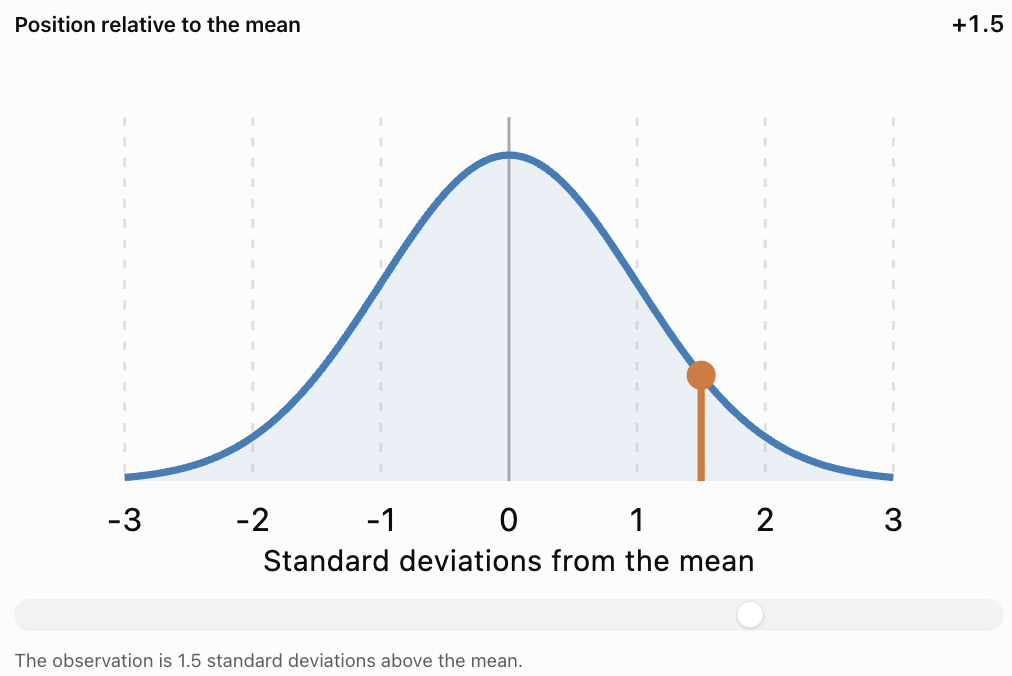
Important Observations
A positive z-score indicates an observation above the mean.
A negative z-score indicates an observation below the mean.
A z-score of zero indicates an observation equal to the mean.
The greater the absolute value of the z-score, the farther the observation is from the mean in standard deviation units.
A z-score has no units because the original units cancel during division.
Comparing Observations Using z-Scores
One of the most useful applications of standard scores is comparing observations from different distributions.
For example, a student may take two examinations with different means and standard deviations.
A raw score of 80 on one examination may represent better relative performance than a score of 90 on another.
Worked Example: Comparing Two Examinations
A student receives the following results:
|
Statistic |
Mathematics |
Science |
|---|---|---|
|
Student's score |
82 |
88 |
|
Class mean |
70 |
80 |
|
Standard deviation |
8 |
10 |
Which examination represents the student's stronger performance relative to the class?
Step 1: Calculate the Mathematics z-Score
z = (82 − 70)/8
z = 12/8
z = 1.5
Step 2: Calculate the Science z-Score
z = (88 − 80)/10
z = 8/10
z = 0.8
Step 3: Compare
Mathematics: z = 1.5
Science: z = 0.8
Interpretation
Although the student's raw Science score is higher, the Mathematics score is farther above its class mean.
Therefore, the student performed better relative to the Mathematics class distribution.
This does not necessarily mean the student understands Mathematics better than Science. It means the Mathematics result occupies a higher standardized position within its reference group.
Comparing Measurements with Different Units
Standard scores can also compare observations measured in different units.
Worked Example: Height and Mass
Suppose an athlete has:
|
Measurement |
Athlete |
Population mean |
Standard deviation |
|---|---|---|---|
|
Height |
190 cm |
175 cm |
10 cm |
|
Mass |
82 kg |
70 kg |
8 kg |
Height z-Score
z = (190 − 175)/10
z = 1.5
Mass z-Score
z = (82 − 70)/8
z = 1.5
Interpretation
The athlete's height and mass are each 1.5 standard deviations above their respective population means.
Even though centimetres and kilograms are different units, z-scores allow us to compare their relative positions.
This is possible because standard scores are dimensionless.
The Standard Normal Distribution
A normal distribution is a continuous, symmetric, bell-shaped probability distribution.
The standard normal distribution has:
-
Mean = 0
-
Standard deviation = 1
Its horizontal axis is measured in z-scores.

Important Properties
For a normal distribution:
-
Approximately 68% of observations lie within one standard deviation of the mean.
-
Approximately 95% lie within two standard deviations.
-
Approximately 99.7% lie within three standard deviations.
This is called the empirical rule or 68–95–99.7 rule.
The empirical rule
68%
Within ±1σ95%
Within ±2σ99.7%
Within ±3σInterpreting Unusual Observations
For a normal distribution:
-
z = 0 represents the mean.
-
z = 1 represents a moderately above-average observation.
-
z = 2 represents an observation relatively far above the mean.
-
z = 3 represents an observation very far above the mean.
Likewise, negative z-scores represent observations below the mean.
A common screening rule is to flag observations with |z| > 2 or |z| > 3 for further investigation.
However, a large absolute z-score does not automatically mean an observation is incorrect.
Connecting z-Scores to Percentiles
Percentiles and z-scores both describe relative position, but they use different scales.
For a normally distributed variable, a z-score can be converted into a percentile using the standard normal cumulative distribution.
Common z-Scores and Percentiles
|
z-score |
Approximate percentile |
|---|---|
|
−3.00 |
0.13th |
|
−2.00 |
2.28th |
|
−1.00 |
15.87th |
|
−0.67 |
25th |
|
0.00 |
50th |
|
+0.67 |
75th |
|
+1.00 |
84.13th |
|
+1.28 |
90th |
|
+1.645 |
95th |
|
+1.96 |
97.5th |
|
+2.00 |
97.72nd |
|
+3.00 |
99.87th |
Worked Example
A student receives a z-score of 1.00 on an examination whose scores are approximately normally distributed.
The corresponding percentile is approximately 84.13.
Interpretation
The student scored higher than approximately 84% of the reference distribution.
This does not mean the student answered 84% of the questions correctly.
It describes relative performance.
Important Limitation
A z-score does not automatically determine a percentile unless we know or assume an appropriate distribution.
For example, a z-score of 1.00 does not always correspond to the 84th percentile in a strongly skewed dataset.
The normal-distribution conversion is valid when the normal model is appropriate.
Calculating a Percentile from a z-Score
A standard normal table, statistical calculator, or spreadsheet can be used to convert z-scores into cumulative probabilities.
The cumulative probability is the area under the standard normal curve to the left of the specified z-score.
Worked Example
Find the approximate percentile corresponding to:
z = 1.25
Step 1: Identify the z-Score
z = 1.25
Step 2: Find the Cumulative Probability
Using a standard normal table:
P(Z ≤ 1.25) ≈ 0.8944
Step 3: Convert to a Percentage
0.8944 × 100% = 89.44%
Final Answer
Approximately the 89.44th percentile
Interpretation
An observation with z = 1.25 lies above approximately 89.44% of a normally distributed reference population.
Calculating a z-Score from a Percentile
We can also work backward.
Suppose a student is at the 90th percentile of a normally distributed examination.
The z-score corresponding to the 90th percentile is approximately:
z = 1.28
If the examination mean is 65 and the standard deviation is 12, estimate the student's score.
Step 1: Start with the z-Score Formula
z = (x − μ)/σ
Step 2: Rearrange
x = μ + zσ
Step 3: Substitute
x = 65 + 1.28(12)
x = 65 + 15.36
x ≈ 80.36
Interpretation
A score of approximately 80.4 corresponds to the 90th percentile under the assumed normal distribution.
The exact score may vary if the actual distribution differs from the normal model.
Standardizing an Entire Dataset
Standardization transforms each observation into a z-score.
For every observation:
z = (x − μ)/σ
Consider a population with:
Mean = 50
Standard deviation = 10
|
Original value |
Calculation |
z-score |
|---|---|---|
|
30 |
(30 − 50)/10 |
−2 |
|
40 |
(40 − 50)/10 |
−1 |
|
50 |
(50 − 50)/10 |
0 |
|
60 |
(60 − 50)/10 |
1 |
|
70 |
(70 − 50)/10 |
2 |
What Happens After Standardization?
For a dataset standardized using its own mean and standard deviation:
-
The standardized mean becomes 0.
-
The standardized standard deviation becomes 1.
-
The relative ordering of observations remains unchanged.
-
The values become unitless.
Standardization does not automatically make a dataset normally distributed.
If the original distribution is skewed, its standardized distribution remains skewed.
Applications in Education
Percentiles and standard scores are widely used to interpret examination results.

Example
Two students complete different standardized examinations.
Student A:
Score = 75
Mean = 60
Standard deviation = 10
Student B:
Score = 85
Mean = 80
Standard deviation = 5
Calculations
Student A:
z = (75 − 60)/10 = 1.5
Student B:
z = (85 − 80)/5 = 1.0
Interpretation
Student A performed better relative to the reference group for their examination.
Standard scores can help compare performance across different tests, provided the reference groups and testing conditions are appropriate.
Applications in Health and Growth
Percentile charts are commonly used to compare children's growth measurements with reference populations of the same age and sex.

For example, a height at the 75th percentile indicates that the measurement is greater than or equal to approximately 75% of measurements in the relevant reference distribution.
Important Considerations
A percentile is not a diagnosis.
A measurement at a high or low percentile is not automatically unhealthy.
Healthcare professionals consider patterns over time, medical history, age, development, and other relevant information.
The choice of reference population matters.
Applications in Sports
Standard scores can help compare athletic performances measured in different units.
For example:
-
Sprint times measured in seconds.
-
Jump heights measured in centimetres.
-
Throwing distances measured in metres.
-
Strength measurements recorded in kilograms.

Worked Example
An athlete runs 100 metres in 11.2 seconds.
The reference group has:
Mean time = 12.0 seconds
Standard deviation = 0.4 seconds
Calculate:
z = (11.2 − 12.0)/0.4
z = −0.8/0.4
z = −2
Interpretation
The athlete's time is two standard deviations below the mean.
Because a lower sprint time is better, this represents an unusually strong performance.
Important Observation
A positive z-score does not always represent a better result.
Its meaning depends on the variable.
For examination scores, higher is often better.
For race times, lower is often better.
Applications in Manufacturing
Manufacturers use standardized measurements to monitor product consistency.
Suppose a factory produces metal rods with:
Mean length = 100 cm
Standard deviation = 0.5 cm
A rod measures 101.2 cm.
Calculate the z-Score
z = (101.2 − 100)/0.5
z = 1.2/0.5
z = 2.4
Interpretation
The rod is 2.4 standard deviations longer than the mean.
This may justify checking the rod against manufacturing tolerances.
However, a z-score alone does not determine whether a product meets specifications.
The acceptable range must be defined separately.
Comparing Percentiles and z-Scores
|
Feature |
Percentile |
z-score |
|---|---|---|
|
Describes |
Relative rank |
Distance from mean |
|
Scale |
Usually 0–100 |
Can be negative or positive |
|
Uses standard deviation |
Not necessarily |
Yes |
|
Mean position |
Not always 50th percentile |
Always z = 0 |
|
Works with skewed data |
Yes |
Yes |
|
Directly gives normal percentile |
Not applicable |
Only with normal model |
|
Useful for |
Rankings and relative positions |
Standardized comparisons |
|
Example |
90th percentile |
z = 1.28 |
Choosing the Correct Measure
Use a percentile when you want to know how an observation ranks relative to other observations.
Use a z-score when you want to know how far an observation is from the mean in standard deviation units.
Both can be useful when comparing observations across groups, but the reference populations must be appropriate.
Common Mistakes
Confusing percentile with percentage
A percentile describes rank, not the proportion of questions answered correctly.
Forgetting to order the dataset
Percentile calculations require data arranged in ascending order.
Assuming all percentile methods give identical results
Different methods can produce slightly different sample percentile values.
Confusing percentile value with percentile rank
A percentile value is a measurement. A percentile rank is a relative position.
Subtracting the observation from the mean
The z-score formula uses x − μ, not μ − x.
Ignoring negative z-scores
Negative z-scores indicate values below the mean.
Assuming a positive z-score is always better
For variables such as race times or error counts, lower values may be preferable.
Confusing standard deviation with variance
Variance uses squared units; standard deviation uses the original units.
Assuming standardized data are normally distributed
Standardization changes location and scale, not the overall distribution shape.
Using normal-distribution percentiles for every dataset
The conversion between z-scores and normal percentiles requires a suitable normal model.
Rounding too early
Keep sufficient precision during calculations and round the final answer.
Ignoring the reference group
A percentile or z-score only has meaning relative to the distribution used to calculate it.
Key Terms
-
Percentile: Value associated with a specified cumulative position in an ordered distribution.
-
Percentile Rank: Relative position of an observation expressed as a percentage.
-
Percentage: Proportion expressed out of 100.
-
Median: Middle value of an ordered dataset; the 50th percentile.
-
Quartile: Value dividing ordered data into four approximately equal groups.
-
Interquartile Range: Difference between the third and first quartiles.
-
Interpolation: Estimation of a value between two known values.
-
Mean: Arithmetic average of a dataset.
-
Standard Deviation: Measure of the spread of observations around the mean.
-
Variance: Average squared deviation from the mean, using the appropriate population or sample formula.
-
Standard Score: Standardized measure of an observation's relative position.
-
z-Score: Number of standard deviations an observation lies above or below the mean.
-
Standardization: Transformation of observations into standardized values.
-
Normal Distribution: Symmetric, bell-shaped probability distribution.
-
Standard Normal Distribution: Normal distribution with mean 0 and standard deviation 1.
-
Cumulative Probability: Probability that a variable is at or below a specified value.
-
Empirical Rule: Approximate 68–95–99.7 pattern for normally distributed observations.
-
Outlier: Observation unusually far from the main body of a dataset.
-
Reference Population: Group used to interpret or compare an observation.
-
Skewed Distribution: Distribution that is asymmetric.
-
Raw Score: Original, unstandardized observation.
-
Relative Position: Location of an observation compared with others.
-
Dimensionless Quantity: Quantity without physical units.
Key Takeaways
-
Percentiles describe relative positions within distributions.
-
The 50th percentile is the median.
-
Quartiles correspond to the 25th, 50th, and 75th percentiles.
-
Percentiles and percentages are not the same.
-
Sample percentiles can be calculated using several accepted conventions.
-
A z-score measures distance from the mean in standard deviation units.
-
The population z-score formula is z = (x − μ)/σ.
-
Positive z-scores indicate observations above the mean.
-
Negative z-scores indicate observations below the mean.
-
A z-score of zero represents the mean.
-
Standard scores allow comparisons across different measurement scales.
-
Standardized observations are unitless.
-
A standard normal distribution has mean 0 and standard deviation 1.
-
Approximately 68%, 95%, and 99.7% of normally distributed observations lie within one, two, and three standard deviations of the mean.
-
Normal-distribution percentiles can be estimated from z-scores when a normal model is appropriate.
-
Percentiles and z-scores must always be interpreted in relation to their reference distributions.
Check Your Understanding
Percentiles
-
Define a percentile.
-
Explain the difference between a percentile and a percentage.
-
What percentile corresponds to the median?
-
Identify the percentiles represented by Q₁ and Q₃.
-
Using L = (k/100)(n + 1), find the position of the 30th percentile in a dataset containing 19 observations.
-
Using the same method, find the 25th percentile of 4, 8, 12, 16, 20, 24, 28.
-
Find the median of 10, 14, 18, 22, 26, 30.
-
If Q₁ = 18 and Q₃ = 42, calculate the IQR.
z-Scores
-
Write the population z-score formula.
-
Calculate the z-score for x = 85, μ = 70, σ = 10.
-
Calculate the z-score for x = 45, μ = 60, σ = 5.
-
What does z = 0 mean?
-
What does z = −1.5 mean?
-
An examination has mean 65 and standard deviation 8. Find the z-score for a score of 81.
-
A value has z = 2, mean 40, and standard deviation 6. Find the original value.
Comparing Observations
-
Student A has z = 1.2 and Student B has z = 0.8. Who performed better relative to their reference group, assuming higher scores are better?
-
Explain why a score of 80 may represent stronger relative performance than a score of 90.
-
Approximately what percentile corresponds to z = 1 in a normal distribution?
-
Does converting data to z-scores make the distribution normal?
-
Explain why a negative z-score may represent excellent performance in a running race.
Answer Key
|
Question |
Answer |
|---|---|
|
1 |
A value describing a specified relative position within a distribution |
|
2 |
Percentage describes a proportion; percentile describes relative position |
|
3 |
50th percentile |
|
4 |
Q₁ = 25th; Q₃ = 75th |
|
5 |
L = 0.30 × 20 = 6 |
|
6 |
L = 0.25 × 8 = 2; P₂₅ = 8 |
|
7 |
(18 + 22)/2 = 20 |
|
8 |
24 |
|
9 |
z = (x − μ)/σ |
|
10 |
1.5 |
|
11 |
−3 |
|
12 |
Observation equals the mean |
|
13 |
1.5 standard deviations below the mean |
|
14 |
2 |
|
15 |
52 |
|
16 |
Student A |
|
17 |
The examinations may have different means and standard deviations |
|
18 |
Approximately 84th percentile |
|
19 |
No |
|
20 |
Lower times are better, so a negative z-score may indicate a faster-than-average time |
Extended Challenge
Percentile Calculations
Use the (n + 1) position method with interpolation for Questions 1–5.
-
Find the 25th percentile of 5, 10, 15, 20, 25, 30, 35, 40, 45.
-
Find the 75th percentile of the same dataset.
-
Calculate the IQR of the dataset.
-
Find the 60th percentile of 12, 15, 18, 22, 25, 29, 34, 38, 42.
-
Explain why two statistical programs may report slightly different percentiles for the same dataset.
Standard Scores
-
Calculate the z-score for x = 92, μ = 75, σ = 10.
-
Calculate the z-score for x = 48, μ = 60, σ = 8.
-
A value has z = −1.25, mean 100, and standard deviation 16. Find the original value.
-
A dataset has mean 50 and standard deviation 12. Determine the values corresponding to z = −2 and z = 2.
-
Explain why z-scores are dimensionless.
Comparing Data
-
A student scores 78 on a test with mean 65 and standard deviation 10. On another test, the student scores 84 with mean 75 and standard deviation 6. Compare the performances.
-
Two athletes complete different events. Athlete A has z = −1.8 for race time. Athlete B has z = 1.5 for jump height. Explain how both results may represent strong performances.
-
A manufacturing process has mean 250 g and standard deviation 4 g. Calculate the z-score of a 261 g product.
-
Explain why the same raw score can have different z-scores in different distributions.
-
Describe a situation in which percentiles would be more useful than raw scores.
Normal Distribution Applications
-
Approximately what percentage of a normal distribution lies within one standard deviation of the mean?
-
Approximately what percentage lies outside two standard deviations?
-
A normal distribution has mean 100 and standard deviation 15. Find the values corresponding to z = −1 and z = 1.
-
Estimate the 90th-percentile value for a normal distribution with mean 50 and standard deviation 8, using z ≈ 1.28.
-
Explain why the normal model should not automatically be used for highly skewed data.
Final Investigation: Comparing Examination Results
Three classes complete different examinations.
|
Statistic |
Class A |
Class B |
Class C |
|---|---|---|---|
|
Mean |
65 |
72 |
58 |
|
Standard deviation |
10 |
8 |
12 |
|
Selected student's score |
80 |
84 |
76 |
Complete the investigation.
-
Calculate the z-score for the student in Class A.
-
Calculate the z-score for the student in Class B.
-
Calculate the z-score for the student in Class C.
-
Rank the students according to raw examination scores.
-
Rank the students according to standardized scores.
-
Explain why the two rankings may differ.
-
Identify which student performed best relative to their class.
-
Identify which student achieved the highest raw score.
-
Explain the role of the mean in standardization.
-
Explain the role of standard deviation.
-
Estimate the normal-distribution percentile for each student, assuming the scores are approximately normally distributed.
-
Explain why the percentile estimates depend on the normality assumption.
-
Determine the raw score corresponding to z = 2 in each class.
-
Determine the raw score corresponding to z = −1 in each class.
-
Explain why a student with z = 0 is not necessarily performing poorly.
-
Describe how a highly skewed distribution could affect interpretation.
-
Explain how standard scores could help compare results from different examinations.
-
Discuss one limitation of using only z-scores to evaluate students.
-
Suggest another statistic that would help describe each class.
-
Write a conclusion explaining why percentiles and standard scores are valuable tools for interpreting educational data.
4. Shape of Distributions
Learning outcomes
- I can identify symmetric distributions.
- I can identify skewed distributions.
- I can recognise outliers.
- I can interpret distribution shape.
- I can compare different datasets.
Shape of Distributions
Introduction
When analysing data, it is important to understand not only the individual values but also how those values are distributed.
The shape of a distribution describes how frequently different values occur and how those values are arranged across a dataset.
Two datasets may have the same mean or median but very different distributions. One might be symmetrical, another might be strongly skewed, and another might contain unusual observations called outliers.
Understanding distribution shape helps us:
-
Recognise patterns in data.
-
Identify symmetric and skewed distributions.
-
Detect unusual observations.
-
Interpret measures such as the mean, median, and standard deviation.
-
Compare datasets more accurately.
-
Decide which statistical measures best describe the data.
Distribution shapes are used in education, economics, medicine, environmental science, manufacturing, and many other fields.


What Is a Distribution?
A distribution describes how the values of a variable are spread across a dataset.
Consider the following examination scores:
45, 52, 58, 63, 67, 70, 72, 75, 79, 84, 91
We can analyse these scores by asking:
-
Where are most of the scores concentrated?
-
Are the scores spread evenly?
-
Are there more high scores or low scores?
-
Are any scores unusually far from the others?
-
Does the distribution have one peak or several peaks?
The answers help us understand the shape of the distribution.
Frequency Distributions
A frequency distribution records how often values or groups of values occur.
For example:
|
Score range |
Frequency |
|---|---|
|
40–49 |
1 |
|
50–59 |
2 |
|
60–69 |
2 |
|
70–79 |
4 |
|
80–89 |
1 |
|
90–99 |
1 |
This table shows that the greatest concentration of scores is between 70 and 79.
A histogram can make the pattern easier to recognise.
Using Histograms to Examine Shape
A histogram displays the frequencies of numerical data grouped into intervals.
The horizontal axis represents numerical intervals.
The vertical axis represents frequency.
Unlike a typical bar chart for categories, histogram bars normally touch because the intervals represent a continuous numerical scale.
Example
Consider the following grouped data:
|
Value range |
Frequency |
|---|---|
|
0–9 |
2 |
|
10–19 |
5 |
|
20–29 |
9 |
|
30–39 |
6 |
|
40–49 |
3 |
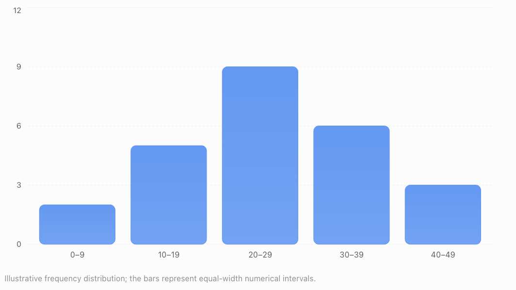
Most observations occur near the middle of the range.
There are fewer observations at the lower and upper ends.
Important Features to Examine
When studying a histogram, look for:
-
Centre: Where the typical values are located.
-
Spread: How widely the observations vary.
-
Shape: Whether the distribution is symmetric or skewed.
-
Peaks: Where observations are most concentrated.
-
Gaps: Intervals containing few or no observations.
-
Outliers: Observations unusually distant from the rest.
These features provide a more complete description than the mean alone.
Symmetric Distributions
A symmetric distribution has approximately the same shape on both sides of its centre.
If the distribution were folded vertically through its centre, the two sides would approximately match.
Symmetric distributions have balanced left and right tails.
Example
Consider:
2, 4, 6, 8, 10, 12, 14
The values are evenly arranged around 8.
The mean is:
(2 + 4 + 6 + 8 + 10 + 12 + 14)/7 = 8
The median is also 8.
This dataset is symmetric around 8.
A Symmetric Frequency Distribution
|
Value |
Frequency |
|---|---|
|
1 |
1 |
|
2 |
3 |
|
3 |
6 |
|
4 |
9 |
|
5 |
6 |
|
6 |
3 |
|
7 |
1 |
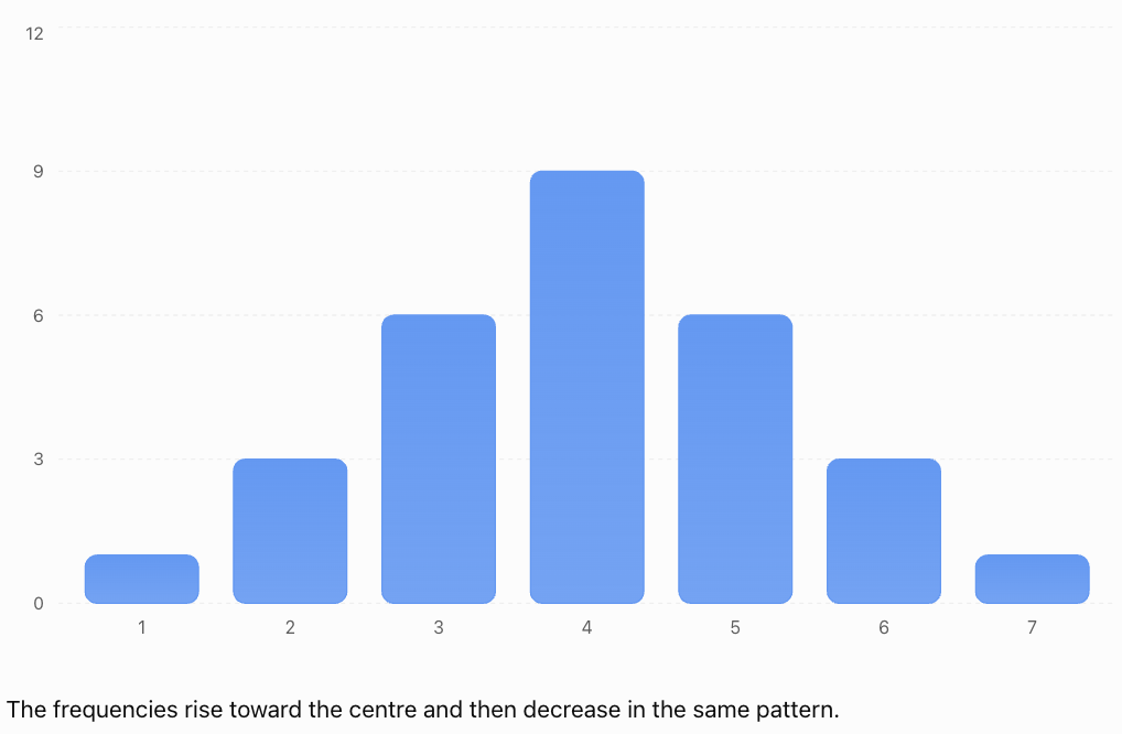
The frequencies rise toward the centre and then decrease in the same pattern.
Characteristics of Symmetric Distributions
-
The left and right sides have similar shapes.
-
The tails are approximately balanced.
-
The mean and median are often close together.
-
A symmetric distribution may have one peak, multiple peaks, or a flat shape.
Important: Symmetry does not automatically mean the distribution is normal or bell-shaped.
The Normal Distribution
One important symmetric distribution is the normal distribution.
It is often called the bell-shaped distribution because of its characteristic appearance.
Characteristics
A normal distribution:
-
Is symmetric around its mean.
-
Has one central peak.
-
Has mean, median, and mode at the same location.
-
Has tails that extend in both directions.
-
Has a shape determined by its mean and standard deviation.
Many measurements are approximately normal under suitable conditions, although real datasets are rarely perfectly normal.
Examples may include some measurement errors and certain biological characteristics within appropriately defined populations.
The Empirical Rule
For a normal distribution:
-
Approximately 68% of observations lie within one standard deviation of the mean.
-
Approximately 95% lie within two standard deviations.
-
Approximately 99.7% lie within three standard deviations.
This is known as the 68–95–99.7 rule.
It applies to normal distributions, not automatically to every symmetric distribution.
Uniform Distributions
A uniform distribution has approximately equal frequencies across its possible values or intervals.
For example, a fair six-sided die has an equal probability of producing each number from 1 to 6.
The theoretical probabilities are:
|
Outcome |
Probability |
|---|---|
|
1 |
1/6 |
|
2 |
1/6 |
|
3 |
1/6 |
|
4 |
1/6 |
|
5 |
1/6 |
|
6 |
1/6 |
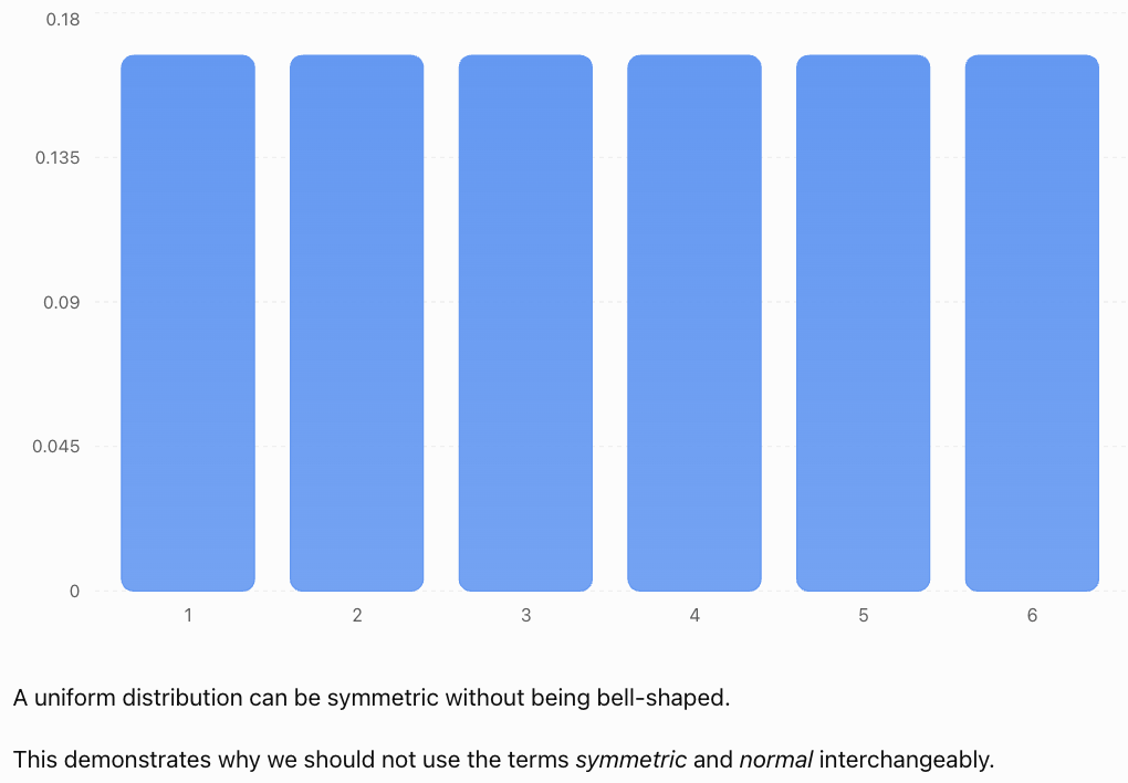
Skewed Distributions
A skewed distribution is asymmetric.
One side extends farther than the other, producing a longer tail.
There are two main types:
-
Right-skewed distributions.
-
Left-skewed distributions.
The direction of skewness is named after the direction of the longer tail, not the location of the tallest bars.
Right-Skewed Distributions
A right-skewed distribution, also called a positively skewed distribution, has a longer tail extending toward larger values.
Most observations are concentrated toward the lower end.
A smaller number of large observations extend the distribution to the right.
Example: Household Incomes
In many populations, most households earn low-to-middle incomes relative to a smaller number of very high-income households.

Example Dataset
20, 22, 23, 24, 25, 26, 28, 32, 80
Most values are between 20 and 32.
The value 80 is much larger than the others.
Calculate the Mean
Sum = 280
Mean = 280/9
Mean ≈ 31.11
Find the Median
There are nine observations.
The fifth value is 25.
Median = 25
The mean is larger than the median because the unusually high value pulls the mean upward.
Characteristics
-
Most values are concentrated toward the left.
-
The tail extends toward the right.
-
Large values may increase the mean.
-
The mean is often greater than the median.
Important Qualification
Mean > median is a common pattern in right-skewed distributions, but it is not a guaranteed rule for every possible dataset.
Distribution shape should be judged primarily from the data or graph, not only by comparing two summary statistics.
Left-Skewed Distributions
A left-skewed distribution, also called a negatively skewed distribution, has a longer tail extending toward smaller values.
Most observations are concentrated toward the higher end.
A smaller number of low observations extend the distribution to the left.
Example: An Easy Examination
Suppose most students score highly on an examination, but a few students receive much lower marks.
The distribution may be left-skewed.
Example Dataset
20, 68, 72, 74, 76, 78, 79, 80, 82
Calculate the Mean
Sum = 629
Mean = 629/9
Mean ≈ 69.89
Find the Median
The fifth value is 76.
Median = 76
The mean is smaller than the median because the low value pulls the mean downward.
Characteristics
-
Most observations are concentrated toward the right.
-
The tail extends toward the left.
-
Low values may decrease the mean.
-
The mean is often less than the median.
Comparing Symmetric and Skewed Distributions
Symmetric
Balanced tailsRight-skewed
Long right tailLeft-skewed
Long left tail|
Feature |
Symmetric |
Right-skewed |
Left-skewed |
|---|---|---|---|
|
Shape |
Balanced |
Longer right tail |
Longer left tail |
|
Concentration |
Often near centre |
Often toward lower values |
Often toward higher values |
|
Mean and median |
Often similar |
Mean often higher |
Mean often lower |
|
Example |
Some measurement errors |
Income data |
Scores on an easy test |
Remember
The direction of skewness is determined by the longer tail.
Understanding Outliers
An outlier is an observation that lies unusually far from the main group of data.
Outliers may be much higher or much lower than most observations.
Example
Consider:
12, 13, 14, 15, 15, 16, 17, 18, 65
Most values are between 12 and 18.
The value 65 is unusually large.
It is a possible outlier.

Possible Causes of Outliers
Outliers may result from:
-
Measurement errors.
-
Data entry mistakes.
-
Unusual but genuine observations.
-
Equipment problems.
-
Rare events.
-
Natural variation.
-
Observations from a different population.
Important Observation
An outlier is not necessarily an error.
A very high examination score, an unusually tall person, or an extreme weather event may be genuine.
Outliers should be investigated before deciding whether to exclude them.
Identifying Outliers Using the IQR Method
One common method uses the interquartile range.
The interquartile range measures the spread of the middle 50% of the data.
IQR = Q₃ − Q₁
Potential outliers are identified using two boundaries called fences.
Lower Fence
Lower fence = Q₁ − 1.5 × IQR
Upper Fence
Upper fence = Q₃ + 1.5 × IQR
Values below the lower fence or above the upper fence are flagged as potential outliers.
Worked Example
Consider:
4, 5, 6, 7, 8, 9, 10, 11, 12, 30
Step 1: Find the Median
Median = (8 + 9)/2
Median = 8.5
Step 2: Find the Quartiles
Using the median-of-halves convention:
Lower half:
4, 5, 6, 7, 8
Q₁ = 6
Upper half:
9, 10, 11, 12, 30
Q₃ = 11
Step 3: Calculate the IQR
IQR = 11 − 6
IQR = 5
Step 4: Calculate the Fences
Lower fence = 6 − 1.5(5)
Lower fence = −1.5
Upper fence = 11 + 1.5(5)
Upper fence = 18.5
Step 5: Identify Outliers
Any value below −1.5 or above 18.5 is flagged.
The value 30 is above 18.5.
Therefore, 30 is a potential outlier.
Important Note
There are several accepted methods for calculating quartiles. The median-of-halves convention is used in this example. Different quartile conventions may produce slightly different fences, particularly for small datasets.
Identifying Unusual Values Using z-Scores
Another method uses standardized scores.
The z-score formula is:
z = (x − μ)/σ
A z-score describes how many standard deviations an observation lies above or below the mean.
Common Screening Guidelines
-
|z| > 2 may indicate an unusually distant observation.
-
|z| > 3 is sometimes used to flag more extreme observations.
These are guidelines, not universal definitions of outliers.
Worked Example
A dataset has:
Mean = 50
Standard deviation = 10
An observation has value 85.
Calculate:
z = (85 − 50)/10
z = 35/10
z = 3.5
The observation is 3.5 standard deviations above the mean.
It may be considered unusually high.
Limitations
The mean and standard deviation can themselves be affected by extreme observations.
For strongly skewed datasets, IQR-based methods may be more appropriate than simple z-score thresholds.
How Outliers Affect the Mean and Median
Outliers can strongly affect some measures of centre.
Consider:
10, 12, 14, 16, 18
Original Mean
Mean = (10 + 12 + 14 + 16 + 18)/5
Mean = 70/5
Mean = 14
Original Median
Median = 14
Now replace the final value, 18, with 100.
New dataset:
10, 12, 14, 16, 100
New Mean
Mean = 152/5
Mean = 30.4
New Median
Median = 14
Interpretation
The mean increases substantially from 14 to 30.4.
The median remains unchanged.
This shows that:
-
The mean is sensitive to extreme values.
-
The median is more resistant to extreme values.
For skewed distributions or datasets containing outliers, the median may better represent a typical observation.
Choosing Between Mean and Median
The most appropriate measure of centre depends on the distribution.
Symmetric Distributions
For approximately symmetric distributions without extreme outliers, the mean is often a useful measure of centre.
Skewed Distributions
For strongly skewed distributions, the median is often more representative.
Distributions with Outliers
The median is usually less affected by extreme observations.
Example: Household Income
Suppose five households earn:
$35,000, $40,000, $45,000, $50,000, $500,000
The mean is:
(35,000 + 40,000 + 45,000 + 50,000 + 500,000)/5
Mean = $134,000
The median is:
$45,000
The median gives a better indication of the income of a typical household in this small group.
The mean is much higher because of one unusually large income.
Unimodal, Bimodal, and Multimodal Distributions
The number of peaks is another important feature of distribution shape.
A mode is a value or category with the highest frequency.
Unimodal Distribution
A unimodal distribution has one main peak.
Many approximately normal distributions are unimodal.
Bimodal Distribution
A bimodal distribution has two distinct peaks.
This may occur when data come from two different groups.
Multimodal Distribution
A multimodal distribution has more than two peaks.

Example: Two Student Groups
Suppose one group of students scores mainly between 40 and 50, while another group scores mainly between 80 and 90.
Combining the results may produce two peaks.
This could indicate two distinct groups within the dataset.
Important Observation
A bimodal distribution is not necessarily skewed.
A distribution can have two peaks and still be symmetric.
Skewness and number of peaks describe different characteristics.
Gaps and Clusters
Distribution shape can also reveal gaps and clusters.
Clusters
A cluster is a region where many observations are concentrated.
For example:
12, 13, 14, 15, 16, 45, 46, 47, 48
There are two clusters:
-
One near 14.
-
Another near 47.
Gaps
A gap is a region containing few or no observations.
In the example above, there are no observations between 16 and 45.
Interpretation
Clusters and gaps may indicate:
-
Different populations.
-
Different experimental conditions.
-
Distinct categories within a dataset.
-
Natural groupings.
-
Sampling or measurement effects.
A gap does not automatically indicate a problem with the data.
Comparing Different Datasets
When comparing datasets, it is useful to examine four main characteristics:
Shape, Centre, Spread, and Unusual Features.
A common statistical description uses the acronym SOCS:
-
Shape: Symmetry, skewness, and number of peaks.
-
Outliers: Unusual observations.
-
Centre: Mean or median.
-
Spread: Range, IQR, or standard deviation.
Worked Example
Consider two datasets.
Dataset A:
40, 45, 50, 55, 60
Dataset B:
10, 45, 50, 55, 90
Step 1: Compare the Means
Dataset A:
Mean = 250/5 = 50
Dataset B:
Mean = 250/5 = 50
Both datasets have the same mean.
Step 2: Compare the Medians
Dataset A median = 50
Dataset B median = 50
Both datasets have the same median.
Step 3: Compare the Ranges
Dataset A:
Range = 60 − 40 = 20
Dataset B:
Range = 90 − 10 = 80
Interpretation
Both datasets have the same centre.
However, Dataset B is much more spread out.
This demonstrates why measures of centre alone cannot fully describe a distribution.
Comparing Distributions with Box Plots
A box plot, also called a box-and-whisker plot, displays the median, quartiles, and spread of a dataset.
Modified box plots also identify potential outliers separately.

Important Features
A box plot can show:
-
The median.
-
The first quartile.
-
The third quartile.
-
The interquartile range.
-
The whiskers.
-
Potential outliers.
Comparing Two Box Plots
When comparing box plots, ask:
-
Which dataset has the higher median?
-
Which dataset has the larger IQR?
-
Which dataset has the greater overall spread?
-
Are there any outliers?
-
Is one side of a box or whisker noticeably longer?
Important Limitation
A box plot provides useful information about centre and spread, but it does not directly reveal the number of peaks.
Two datasets with very different histogram shapes can sometimes have similar box plots.
How Sample Size Affects Distribution Shape
Small datasets may appear irregular even when sampled from a symmetric population.
For example, a sample of ten heights may show an uneven pattern.
A sample of several thousand heights may reveal a clearer overall shape.
Why?
Random variation has a stronger visible effect in small samples.
As sample size increases, the observed distribution may more closely resemble the underlying population distribution.
However, a larger sample does not automatically correct biased sampling.
A large biased sample can still give a misleading picture.
How Histogram Intervals Affect Shape
The apparent shape of a histogram can change depending on the interval width.
Very wide intervals may hide important patterns.
Very narrow intervals may make a distribution appear irregular or noisy.
Example
Suppose examination scores range from 0 to 100.
Using intervals of width 50 produces only two bars.
Using intervals of width 10 produces ten bars.
The second histogram may reveal more detail about clusters, skewness, or outliers.
Important Conclusion
Histogram shape should be interpreted with consideration of the interval widths and the number of observations.
When comparing histograms, consistent interval widths are especially helpful.
Real-World Application: Examination Results
Examination results can have different distribution shapes depending on test difficulty.

Difficult Examination
Most students may score relatively low, while a few score highly.
The distribution may be right-skewed.
Easy Examination
Most students may score highly, while a few score much lower.
The distribution may be left-skewed.
Moderately Difficult Examination
Scores may cluster around the middle.
The distribution may be approximately symmetric.
Interpretation
Distribution shape can provide useful feedback about an assessment.
However, shape alone does not determine whether a test is valid, fair, or appropriately challenging.
Other factors, such as question quality and the abilities of the students, must also be considered.
Real-World Application: Income Distributions
Income distributions are often right-skewed.

Most incomes may be concentrated in a lower or middle range, while a smaller number of very high incomes create a long right tail.
Why Does This Matter?
The mean income may be substantially higher than the median income.
When describing typical income, the median is often more informative.
However, the mean remains useful for calculations involving total income.
Both statistics have legitimate uses.
Real-World Application: Environmental Data
Environmental measurements may have skewed distributions.
Examples include:
-
Daily rainfall amounts.
-
River flow rates.
-
Air pollutant concentrations.
-
Storm intensities.
-
Certain soil contaminant measurements.

Example: Daily Rainfall
Many days may have little or no rainfall.
A smaller number of days may experience very heavy rainfall.
This can produce a right-skewed distribution.
Interpretation
A few extreme rainfall events can strongly increase the mean.
The median may be zero in locations with many dry days.
For environmental planning, both typical conditions and extreme observations may be important.
Real-World Application: Manufacturing Quality Control
Manufacturers monitor the distribution of product measurements.
 wQI6-jisIRlogp3oymKZba5mnc9mXGz426qzidVhdFh8AoCnsn60YpqhbjarVIGv7XJ31I0VDKHkGZVTHx7MQX_6HuRMYXhVEz1MV2IZO4nyLW1YVDUUv_ER3huob9-2D4XDusoXD9SupJEHAarcur2UG8Ow8Y?purpose=inline" alt="Quality Control Training Certificate | Free & Fast Course">
Suppose a factory produces bolts intended to have a diameter of 10 mm.
A roughly symmetric distribution centred near 10 mm may indicate a reasonably stable process.
However, if the distribution becomes skewed or develops unusual observations, it may indicate a change in production conditions.
Important Questions
-
Is the distribution centred near the target?
-
Is the spread small enough?
-
Are there unusual measurements?
-
Has the distribution changed over time?
Distribution shape helps identify patterns, but actual acceptance decisions must use specified manufacturing tolerances.
Common Mistakes
Confusing skewness with the location of the peak
Skewness is named after the direction of the longer tail.
Assuming every symmetric distribution is normal
Uniform and bimodal distributions can also be symmetric.
Assuming the mean and median always follow a fixed order
Mean > median is common in right-skewed distributions, but not guaranteed.
Ignoring outliers
Outliers can strongly affect the mean, range, and standard deviation.
Automatically deleting outliers
Unusual observations may be genuine and important.
Using only the mean to compare datasets
Datasets can have the same mean but very different spreads and shapes.
Assuming all data should be normally distributed
Many real-world variables are naturally skewed or multimodal.
Ignoring histogram interval widths
Different bin widths can make the same dataset appear different.
Confusing gaps with outliers
A gap is an empty region. An outlier is an unusually distant observation.
Using the empirical rule for every distribution
The 68–95–99.7 rule applies to normal distributions.
Confusing variability with skewness
A dataset can have a large spread and still be symmetric.
Key Terms
-
Distribution: Arrangement of observations according to their values and frequencies.
-
Distribution Shape: Overall pattern formed by the observations.
-
Symmetric Distribution: Distribution with approximately balanced sides around its centre.
-
Skewed Distribution: Asymmetric distribution with a longer tail on one side.
-
Right-Skewed Distribution: Distribution with a longer tail toward higher values.
-
Left-Skewed Distribution: Distribution with a longer tail toward lower values.
-
Positive Skewness: Another term for right-skewness.
-
Negative Skewness: Another term for left-skewness.
-
Normal Distribution: Symmetric, bell-shaped probability distribution.
-
Uniform Distribution: Distribution with equal or approximately equal frequencies or probabilities across values or intervals.
-
Outlier: Observation unusually far from the main group of data.
-
Mean: Arithmetic average.
-
Median: Middle value of an ordered dataset.
-
Mode: Most frequently occurring value.
-
Range: Difference between the maximum and minimum values.
-
Quartile: Value dividing ordered data into four approximately equal groups.
-
Interquartile Range: Difference between the third and first quartiles.
-
Lower Fence: Q₁ − 1.5 × IQR.
-
Upper Fence: Q₃ + 1.5 × IQR.
-
Histogram: Graph showing the frequency distribution of numerical data.
-
Box Plot: Graph summarising quartiles, median, spread, and possible outliers.
-
Unimodal: Having one main peak.
-
Bimodal: Having two main peaks.
-
Multimodal: Having more than two peaks.
-
Cluster: Group of observations concentrated within a region.
-
Gap: Region with few or no observations.
-
Spread: Extent to which data values vary.
-
Standard Deviation: Measure of dispersion around the mean.
-
z-Score: Number of standard deviations an observation lies above or below the mean.
Key Takeaways
-
Distribution shape describes how observations are arranged.
-
Symmetric distributions have approximately balanced left and right sides.
-
Normal distributions are symmetric and bell-shaped.
-
Not every symmetric distribution is normal.
-
Right-skewed distributions have longer right tails.
-
Left-skewed distributions have longer left tails.
-
Outliers are observations unusually far from the main group.
-
The IQR method can identify potential outliers.
-
Outliers may be genuine and should not automatically be removed.
-
The mean is sensitive to extreme values.
-
The median is more resistant to extreme values.
-
Skewed distributions are often better summarised using the median and IQR.
-
Histograms help reveal shape, peaks, gaps, and clusters.
-
Box plots help compare centres, spreads, and potential outliers.
-
Datasets can have identical means but different shapes and spreads.
-
Comparing distributions requires examining shape, centre, spread, and unusual observations.
Check Your Understanding
Identifying Distribution Shapes
-
Define a symmetric distribution.
-
What is a right-skewed distribution?
-
What is a left-skewed distribution?
-
Is every symmetric distribution normally distributed?
-
What does the direction of skewness describe?
Recognising Outliers
-
Define an outlier.
-
Give two possible causes of outliers.
-
Explain why an outlier should not automatically be removed.
-
Calculate the IQR if Q₁ = 20 and Q₃ = 44.
-
Calculate the upper outlier fence for Q₁ = 20 and Q₃ = 44.
Interpreting Centre and Spread
-
Which measure of centre is generally more resistant to outliers?
-
Why might the mean be higher than the median in a right-skewed distribution?
-
What does a large range indicate?
-
Can two datasets have the same mean but different spreads?
-
Why is the median often useful for income data?
Comparing Distributions
-
What is a bimodal distribution?
-
What is a cluster?
-
What is a gap?
-
Name four characteristics useful when comparing datasets.
-
Explain why histogram interval widths matter.
Answer Key
|
Question |
Answer |
|---|---|
|
1 |
A distribution with approximately balanced sides |
|
2 |
A distribution with a longer right tail |
|
3 |
A distribution with a longer left tail |
|
4 |
No |
|
5 |
Direction of the longer tail |
|
6 |
An unusually distant observation |
|
7 |
Measurement error, rare genuine event, or other reasonable examples |
|
8 |
It may be genuine and important |
|
9 |
24 |
|
10 |
44 + 1.5(24) = 80 |
|
11 |
Median |
|
12 |
Large values can pull the mean upward |
|
13 |
Greater difference between maximum and minimum |
|
14 |
Yes |
|
15 |
It is less affected by extremely high incomes |
|
16 |
A distribution with two main peaks |
|
17 |
Region containing many observations |
|
18 |
Region containing few or no observations |
|
19 |
Shape, centre, spread, and outliers |
|
20 |
They affect how patterns appear in the graph |
Extended Challenge
Symmetry and Skewness
-
Describe the likely shape of a distribution in which most values are low but a few are extremely high.
-
Describe the likely shape of an examination distribution in which most students score near 90%, but a few score below 40%.
-
Explain why a uniform distribution can be symmetric.
-
Describe a situation that might produce a bimodal distribution.
-
Explain why skewness should be determined from the overall shape rather than only from the mean and median.
Outlier Calculations
Use the median-of-halves quartile convention.
-
Find Q₁, Q₃, and the IQR for 2, 4, 6, 8, 10, 12, 14, 16.
-
Calculate the lower and upper fences for the dataset.
-
Determine whether 30 would be flagged as an outlier if added to the dataset.
-
Explain how the mean would change if 30 were added.
-
Explain why the median would be less affected.
Comparing Datasets
Dataset A:
10, 12, 14, 16, 18
Dataset B:
2, 8, 14, 20, 26
-
Calculate the mean of each dataset.
-
Calculate the median of each dataset.
-
Calculate the range of each dataset.
-
Compare the spread of the two datasets.
-
Explain why comparing only the means would be misleading.
Real-World Interpretation
-
Explain why household income distributions are often right-skewed.
-
Describe how outliers may affect environmental measurements.
-
Explain how distribution shape could help teachers analyse examination results.
-
Discuss why a manufacturer might investigate a sudden change in the shape of product measurements.
-
Explain why larger samples may reveal distribution patterns more clearly than smaller samples.
Final Investigation: Comparing Examination Distributions
Three classes complete different examinations.
Class A
45, 50, 55, 60, 65, 70, 75
Class B
20, 60, 65, 68, 70, 72, 75
Class C
45, 48, 50, 52, 55, 58, 95
Complete the investigation.
-
Order each dataset from smallest to largest.
-
Calculate the mean of each class.
-
Calculate the median of each class.
-
Calculate the range of each class.
-
Identify which dataset is symmetric.
-
Describe the likely skewness of Class B.
-
Describe the likely skewness of Class C.
-
Explain how the low score in Class B affects its mean.
-
Explain how the high score in Class C affects its mean.
-
Compare the mean and median of each class.
-
Construct a dot plot for each dataset using the same horizontal scale.
-
Describe the shape of each distribution.
-
Calculate the quartiles using the median-of-halves method.
-
Calculate the IQR for each class.
-
Calculate the outlier fences for each class.
-
Identify any observations flagged as potential outliers.
-
Explain which measure of centre best describes each class.
-
Compare the overall spreads of the three classes.
-
Explain why the same mean would not necessarily indicate similar examination performance.
-
Write a short statistical report comparing the distributions, including their shape, centre, spread, and unusual observations.
5. Box Plots and Histograms
Learning outcomes
- I can construct box plots.
- I can construct histograms.
- I can compare multiple distributions.
- I can identify spread and outliers graphically.
- I can interpret statistical graphs.
Box Plots and Histograms
Introduction
Statistical graphs help us understand how data are organised, distributed, and spread out.
Two particularly useful graphs are box plots and histograms.
A box plot summarises a dataset using its median, quartiles, and overall spread. It is especially useful for comparing different datasets and identifying potential outliers.
A histogram shows how frequently numerical values occur within intervals. It is especially useful for identifying the shape of a distribution, including symmetry, skewness, clusters, and gaps.
Although both graphs describe distributions, they reveal different information.
For example, a histogram can show whether examination scores form one peak or two, while a box plot makes it easier to compare the medians and interquartile ranges of two classes.
Understanding how to construct and interpret these graphs allows us to draw meaningful conclusions from data.


Understanding Box Plots
A box plot, also called a box-and-whisker plot, is a graph that summarises the centre and spread of numerical data.
A traditional box plot is constructed using five important values, called the five-number summary:
-
Minimum
-
First quartile (Q₁)
-
Median (Q₂)
-
Third quartile (Q₃)
-
Maximum
These values divide the dataset into four sections containing approximately 25% of the observations each.
A modified box plot also identifies potential outliers separately.
The Structure of a Box Plot
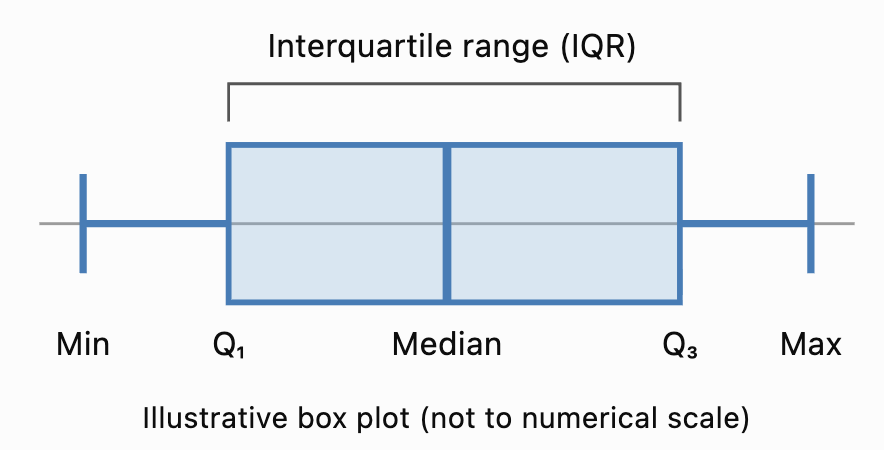
Important Features
The box extends from Q₁ to Q₃.
The line inside the box represents the median.
The length of the box represents the interquartile range.
The whiskers extend toward the lowest and highest values included under the chosen box-plot convention.
In a traditional box plot, the whiskers extend to the minimum and maximum observations.
In a modified box plot, the whiskers extend to the most extreme observations that are not classified as outliers.
The Five-Number Summary
Before constructing a box plot, we need to calculate the five-number summary.
Consider the ordered dataset:
3, 5, 7, 8, 10, 12, 14, 16, 18, 21, 25
Minimum
The smallest value is:
Minimum = 3
Maximum
The largest value is:
Maximum = 25
Median
There are 11 observations.
The median is the sixth value.
Median = 12
First Quartile
Using the median-of-halves method, exclude the median and examine the lower five values:
3, 5, 7, 8, 10
The middle value is 7.
Q₁ = 7
Third Quartile
Examine the upper five values:
14, 16, 18, 21, 25
The middle value is 18.
Q₃ = 18
Five-Number Summary
|
Statistic |
Value |
|---|---|
|
Minimum |
3 |
|
Q₁ |
7 |
|
Median |
12 |
|
Q₃ |
18 |
|
Maximum |
25 |
This summary provides the information needed to construct a traditional box plot.
Note: Several accepted quartile conventions exist. These notes use the median-of-halves method, excluding the overall median when the dataset has an odd number of observations. Other methods may produce slightly different quartiles.
Constructing a Box Plot
Let's construct a box plot for:
4, 6, 8, 10, 12, 14, 16, 18, 20
Step 1: Order the Data
The values are already arranged in ascending order.
Step 2: Identify the Minimum and Maximum
Minimum = 4
Maximum = 20
Step 3: Find the Median
There are nine observations.
The fifth value is 12.
Median = 12
Step 4: Find the Quartiles
Lower half:
4, 6, 8, 10
Q₁ = (6 + 8)/2 = 7
Upper half:
14, 16, 18, 20
Q₃ = (16 + 18)/2 = 17
Step 5: Record the Five-Number Summary
|
Minimum |
Q₁ |
Median |
Q₃ |
Maximum |
|---|---|---|---|---|
|
4 |
7 |
12 |
17 |
20 |
Step 6: Draw a Number Line
Choose a suitable horizontal scale covering the data.
For this example, a scale from 0 to 22 is appropriate.
Step 7: Draw the Box
Draw a rectangle extending from Q₁ = 7 to Q₃ = 17.
Step 8: Mark the Median
Draw a vertical line inside the box at 12.
Step 9: Add the Whiskers
Draw lines extending from the box to the minimum and maximum.
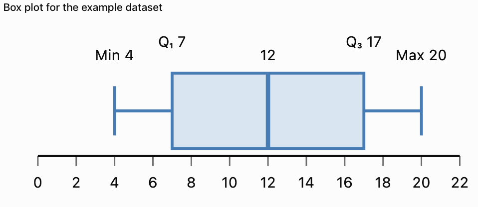
The completed box plot shows the centre and spread of the dataset.
Understanding the Interquartile Range
The interquartile range (IQR) measures the spread of the middle 50% of the observations.
The formula is:
IQR = Q₃ − Q₁
For the previous dataset:
Q₁ = 7
Q₃ = 17
IQR = 17 − 7
IQR = 10
Interpretation
The middle 50% of the observations lie between 7 and 17.
The width of this interval is 10 units.
A smaller IQR indicates that the middle half of the data is more closely grouped.
A larger IQR indicates that the middle half is more widely spread.
Why Is the IQR Useful?
The IQR is resistant to extreme values.
Unlike the range, it is not determined by the smallest and largest observations.
This makes it particularly useful for skewed distributions or datasets containing outliers.
Identifying Outliers Using Box Plots
An outlier is an observation unusually far from the main group of data.
A common method for identifying potential outliers uses the IQR.
Outlier Fences
Lower fence = Q₁ − 1.5 × IQR
Upper fence = Q₃ + 1.5 × IQR
Observations below the lower fence or above the upper fence are flagged as potential outliers.
Worked Example
Consider:
5, 6, 7, 8, 9, 10, 11, 12, 13, 40
Step 1: Find the Median
Median = (9 + 10)/2
Median = 9.5
Step 2: Find Q₁ and Q₃
Lower half:
5, 6, 7, 8, 9
Q₁ = 7
Upper half:
10, 11, 12, 13, 40
Q₃ = 12
Step 3: Calculate the IQR
IQR = 12 − 7
IQR = 5
Step 4: Calculate the Fences
Lower fence = 7 − 1.5(5)
Lower fence = −0.5
Upper fence = 12 + 1.5(5)
Upper fence = 19.5
Step 5: Identify Outliers
The value 40 exceeds the upper fence.
40 is a potential outlier.
Modified Box Plot
In a modified box plot:
-
The box extends from Q₁ = 7 to Q₃ = 12.
-
The median is 9.5.
-
The lower whisker extends to 5.
-
The upper whisker extends to 13.
-
The outlier 40 is shown separately as a point.

Important Observation
An outlier is not necessarily an error.
It may represent a genuine unusual event, an extreme measurement, or a mistake.
Outliers should be investigated before deciding whether they should be excluded.
Interpreting Box Plot Shapes
Box plots can provide clues about the shape of a distribution.
Approximately Symmetric Distribution
In an approximately symmetric distribution:
-
The median is often near the centre of the box.
-
The whiskers may have similar lengths.
-
The two halves of the box may be similar in width.
Right-Skewed Distribution
A right-skewed distribution may have:
-
A longer upper whisker.
-
A median closer to Q₁.
-
High-value outliers.
Left-Skewed Distribution
A left-skewed distribution may have:
-
A longer lower whisker.
-
A median closer to Q₃.
-
Low-value outliers.

Important Limitation
Box plots provide clues about skewness but do not show the complete distribution.
A histogram is generally better for examining detailed distribution shape and identifying multiple peaks.
Comparing Multiple Box Plots
One of the main advantages of box plots is that several datasets can be compared on the same numerical scale.
Suppose two classes complete a mathematics examination.
Class A
50, 55, 60, 65, 70, 75, 80, 85, 90
Class B
40, 45, 50, 65, 70, 75, 90, 95, 100
Calculate the Five-Number Summaries
|
Statistic |
Class A |
Class B |
|---|---|---|
|
Minimum |
50 |
40 |
|
Q₁ |
57.5 |
47.5 |
|
Median |
70 |
70 |
|
Q₃ |
82.5 |
92.5 |
|
Maximum |
90 |
100 |
|
IQR |
25 |
45 |
|
Range |
40 |
60 |
Interpretation
Both classes have the same median score of 70.
However, Class B has a larger IQR and range.
This means the scores in Class B are more widely spread.
Class A has more consistent scores around the centre.
What Should We Compare?
When comparing box plots, examine:
-
Median: Which group has the higher typical value?
-
IQR: Which group has more variation in its middle 50%?
-
Range: Which group has the greater overall spread?
-
Outliers: Are there unusual observations?
-
Shape: Are the quartile intervals and whiskers balanced?
Understanding Histograms
A histogram is a graph that displays the frequency distribution of numerical data.
Histograms group values into intervals called bins or classes.
The horizontal axis shows the numerical intervals.
The vertical axis usually shows frequency.
The bars touch because adjacent intervals represent consecutive parts of a numerical scale.

Example
A teacher records the examination scores of 30 students.
|
Score interval |
Frequency |
|---|---|
|
0–19 |
2 |
|
20–39 |
4 |
|
40–59 |
7 |
|
60–79 |
11 |
|
80–99 |
6 |
|
Total |
30 |
A histogram makes it easier to see where scores are concentrated.
Most students scored between 60 and 79.
Constructing a Histogram
Consider the following 20 measurements:
12, 15, 17, 18, 21, 22, 24, 25, 27, 28, 31, 32, 33, 35, 36, 38, 41, 43, 45, 48
Step 1: Identify the Range
Minimum = 12
Maximum = 48
Range = 48 − 12
Range = 36
Step 2: Choose Intervals
We will use equal-width intervals of 10 units.
-
10–19
-
20–29
-
30–39
-
40–49
For integer data, these can be treated as intervals 10 ≤ x < 20, 20 ≤ x < 30, and so on.
Step 3: Count the Frequencies
|
Interval |
Values |
Frequency |
|---|---|---|
|
10–19 |
12, 15, 17, 18 |
4 |
|
20–29 |
21, 22, 24, 25, 27, 28 |
6 |
|
30–39 |
31, 32, 33, 35, 36, 38 |
6 |
|
40–49 |
41, 43, 45, 48 |
4 |
|
Total |
20 |
Step 4: Draw the Axes
Label the horizontal axis with the measurement intervals.
Label the vertical axis with frequency.
Step 5: Draw the Bars
Each bar represents the frequency of its interval.
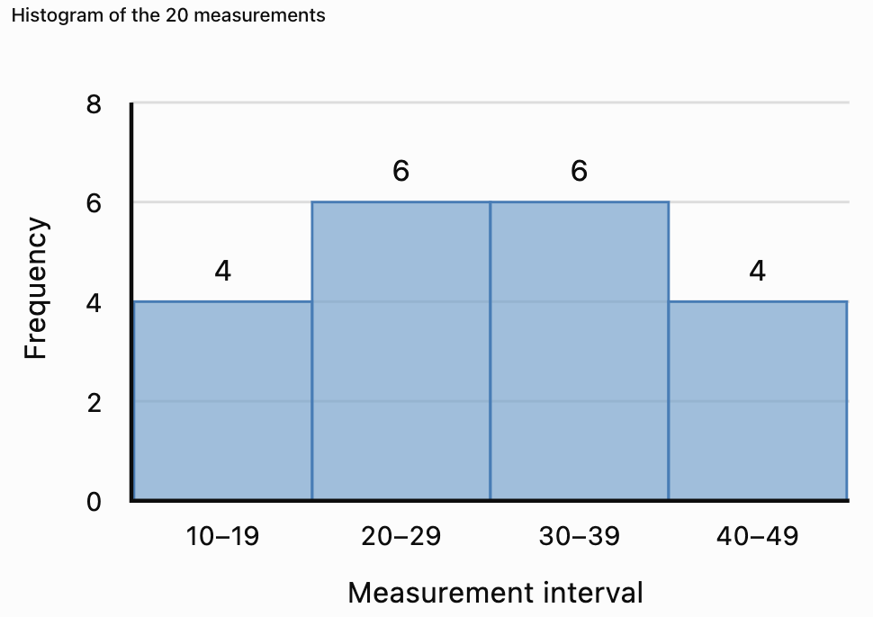
Interpretation
The middle intervals have the highest frequencies.
The frequencies are balanced around the centre.
The distribution appears approximately symmetric.
Histograms Versus Bar Charts
Histograms and bar charts may look similar, but they represent different types of data.
|
Feature |
Histogram |
Bar chart |
|---|---|---|
|
Data type |
Numerical |
Usually categorical |
|
Horizontal axis |
Numerical intervals |
Categories |
|
Bar spacing |
Bars normally touch |
Bars usually have gaps |
|
Bar order |
Numerical order |
May be rearranged |
|
Main purpose |
Show distribution |
Compare categories |
|
Example |
Student heights |
Favourite subjects |
Example
A histogram might display the heights of 100 students.
A bar chart might display how many students prefer Mathematics, Science, English, or History.


Choosing Histogram Intervals
The choice of interval width affects the appearance of a histogram.
Very Wide Intervals
Wide intervals produce fewer bars.
They may hide important details such as gaps or multiple peaks.
Very Narrow Intervals
Narrow intervals produce more bars.
They may reveal additional detail but can make the graph appear irregular.
Appropriate Intervals
A useful histogram should have intervals that:
-
Cover the entire dataset.
-
Do not overlap.
-
Have clearly defined boundaries.
-
Are usually equal in width.
-
Reveal meaningful patterns.
There is no single best interval width for every dataset.
Example
Suppose test scores range from 0 to 100.
Using intervals of width 50 creates only two bars.
Using intervals of width 10 creates ten bars.
The second histogram may reveal more detail about the shape of the distribution.
Unequal Histogram Intervals
Sometimes histograms use intervals of different widths.
In these cases, using frequency directly as bar height can be misleading.
Instead, the bar height should represent frequency density.
Frequency Density Formula
Frequency density = Frequency / Class width
The area of each bar then represents the frequency.
Worked Example
|
Interval |
Width |
Frequency |
Frequency density |
|---|---|---|---|
|
0–10 |
10 |
20 |
2 |
|
10–20 |
10 |
30 |
3 |
|
20–40 |
20 |
40 |
2 |
|
40–80 |
40 |
20 |
0.5 |
Interpretation
The interval 20–40 has the highest total frequency, but it is twice as wide as the first two intervals.
Its frequency density is therefore 2.
A histogram with unequal intervals must account for the different widths.
Remember: For unequal-width histograms, bar area—not bar height alone—represents frequency.
Interpreting Histogram Shapes
Histograms reveal important patterns in numerical data.
Symmetric Distribution
A symmetric histogram has approximately balanced sides.
The frequencies often increase toward the centre and decrease toward both ends.
Right-Skewed Distribution
A right-skewed histogram has a longer tail toward larger values.
Most observations are concentrated toward the lower end.
Left-Skewed Distribution
A left-skewed histogram has a longer tail toward smaller values.
Most observations are concentrated toward the higher end.


Unimodal Distribution
A unimodal distribution has one main peak.
Bimodal Distribution
A bimodal distribution has two main peaks.
This may indicate that the data contain two distinct groups.
Uniform Distribution
A uniform distribution has approximately equal frequencies across its intervals.
Important Observation
Histograms reveal features that box plots may hide.
For example, a box plot may not show that a dataset has two separate peaks.
Identifying Outliers in Histograms
An outlier may appear as an isolated bar or a small group of observations separated from the main distribution.
Example
Suppose most examination scores are between 50 and 90, but one score is 5.
The histogram may show a gap between the low score and the rest of the distribution.
This suggests that the low score should be investigated.
However, a histogram alone does not establish whether a value meets a formal outlier rule.
The appearance also depends on the chosen intervals.
Box Plots Versus Histograms for Outliers
Box plots can use a formal IQR-based rule to identify potential outliers.
Histograms can reveal isolated observations or unusual gaps.
Both are useful, but they provide different kinds of evidence.
Comparing Multiple Histograms
When comparing histograms, examine the shape, centre, spread, and unusual features.
Suppose two classes complete the same examination.
Class A
Most students score between 60 and 80.
The distribution is approximately symmetric.
Class B
Most students score between 40 and 60, but a few students score above 90.
The distribution is right-skewed.
Interpretation
Class A appears to have more consistent results around the middle.
Class B has a larger concentration of lower scores and a small number of high scores.
However, exact comparisons of centre and spread require numerical summaries or more detailed data.
Fair Comparisons
When comparing histograms, it is helpful to use:
-
The same numerical scale.
-
The same interval boundaries.
-
The same interval widths.
-
Relative frequencies when sample sizes differ.
If one class contains 20 students and another contains 200, raw frequency bars may not be directly comparable.
Relative-frequency histograms can solve this problem.
Relative-Frequency Histograms
A relative-frequency histogram shows proportions or percentages rather than raw counts.
Formula
Relative frequency = Frequency / Total observations
To convert to a percentage:
Percentage frequency = (Frequency / Total) × 100%
Worked Example
A class of 40 students receives the following results:
|
Score interval |
Frequency |
Relative frequency |
|---|---|---|
|
0–19 |
2 |
5% |
|
20–39 |
4 |
10% |
|
40–59 |
10 |
25% |
|
60–79 |
16 |
40% |
|
80–99 |
8 |
20% |
|
Total |
40 |
100% |
Interpretation
Forty percent of the class scored between 60 and 79.
Relative-frequency histograms are particularly useful when comparing groups of different sizes.
Box Plots and Histograms: Strengths and Limitations
|
Feature |
Box plot |
Histogram |
|---|---|---|
|
Shows median |
Yes |
Not directly |
|
Shows quartiles |
Yes |
Not directly |
|
Shows IQR |
Yes |
Not directly |
|
Shows overall spread |
Yes |
Yes |
|
Identifies potential outliers |
Yes, using a rule |
Visually suggests them |
|
Shows symmetry or skewness |
Gives clues |
Shows shape more clearly |
|
Shows multiple peaks |
No |
Yes |
|
Shows gaps and clusters |
Limited |
Yes |
|
Compares several datasets |
Very effective |
Effective with consistent scales |
|
Requires interval selection |
No |
Yes |
Which Graph Should We Use?
Use a box plot when the goal is to compare medians, quartiles, spreads, and potential outliers.
Use a histogram when the goal is to examine distribution shape, peaks, clusters, and gaps.
Using both graphs together often provides the clearest understanding.
Real-World Application: Examination Results
Teachers can use box plots and histograms to analyse student performance.

Using a Histogram
A histogram can show:
-
Whether scores cluster near the middle.
-
Whether an examination appears relatively easy or difficult for a group.
-
Whether there are two distinct groups of scores.
-
Whether a few students have unusually low or high results.
Using a Box Plot
A box plot can show:
-
The median score.
-
The middle 50% of results.
-
Differences in spread between classes.
-
Potential outliers.
Interpretation
If two classes have the same median but different IQRs, they have similar central scores but different levels of variability.
The class with the smaller IQR has a more tightly grouped middle half of scores.
Real-World Application: Manufacturing
A factory produces metal components with a target diameter of 20 mm.

A histogram can reveal whether most components are close to the target diameter.
A box plot can compare the spread of measurements from different production machines.
Example
Machine A:
Median diameter = 20.0 mm
IQR = 0.2 mm
Machine B:
Median diameter = 20.0 mm
IQR = 0.8 mm
Both machines have the same median.
However, Machine A has a smaller IQR.
Its middle 50% of measurements are more consistent.
This does not by itself establish whether either machine meets the required tolerances.
Real-World Application: Environmental Measurements
Environmental scientists may use histograms to examine rainfall, temperature, or air-quality measurements.

Rainfall Example
A histogram of daily rainfall may show many days with little rainfall and a few days with very heavy rainfall.
This produces a right-skewed distribution.
A box plot can help identify unusually wet days.
Interpretation
Extreme observations may be important for planning drainage systems, managing flood risk, and understanding environmental variability.
Removing unusual values without investigation could eliminate important information.
Common Mistakes
Forgetting to order data before finding quartiles
Quartiles must be calculated from ordered observations.
Confusing the median with the mean
The line inside a standard box plot represents the median, not necessarily the mean.
Drawing whiskers to outliers in a modified box plot
Modified box plots show potential outliers separately.
Assuming the box represents all observations
The box represents the middle 50% of the distribution.
Confusing IQR with range
IQR = Q₃ − Q₁.
Range = Maximum − Minimum.
Using overlapping histogram intervals
Each observation should belong to exactly one interval.
Leaving gaps between histogram bars
For consecutive numerical intervals, histogram bars normally touch.
Using unequal intervals without frequency density
Unequal-width histograms require bar heights that account for interval widths.
Confusing histogram and bar chart data
Histograms display numerical distributions; bar charts usually compare categories.
Assuming a box plot reveals every feature of the distribution
Box plots do not directly reveal multiple peaks or detailed clusters.
Comparing graphs with different scales carelessly
Different scales can make similar distributions appear very different.
Assuming an isolated bar proves an outlier
Histogram appearance depends on interval selection.
Key Terms
-
Box Plot: Graph summarising the centre and spread of numerical data.
-
Box-and-Whisker Plot: Another name for a box plot.
-
Five-Number Summary: Minimum, Q₁, median, Q₃, and maximum.
-
Minimum: Smallest observation.
-
Maximum: Largest observation.
-
Median: Middle value of ordered data.
-
First Quartile (Q₁): Value separating approximately the lowest 25% of observations.
-
Third Quartile (Q₃): Value separating approximately the lowest 75% of observations.
-
Interquartile Range (IQR): Difference between Q₃ and Q₁.
-
Range: Difference between the maximum and minimum.
-
Whisker: Line extending from a box toward the extremes of the data under the chosen convention.
-
Outlier: Observation unusually far from the main group.
-
Lower Fence: Q₁ − 1.5 × IQR.
-
Upper Fence: Q₃ + 1.5 × IQR.
-
Histogram: Graph displaying the frequency distribution of numerical data.
-
Frequency: Number of observations in a category or interval.
-
Relative Frequency: Proportion of observations in an interval.
-
Class Interval: Numerical interval used to group observations.
-
Bin: Another term for a histogram interval.
-
Class Width: Numerical width of an interval.
-
Frequency Density: Frequency divided by interval width.
-
Symmetric Distribution: Distribution with approximately balanced sides.
-
Right-Skewed Distribution: Distribution with a longer right tail.
-
Left-Skewed Distribution: Distribution with a longer left tail.
-
Unimodal Distribution: Distribution with one main peak.
-
Bimodal Distribution: Distribution with two main peaks.
-
Cluster: Region containing many observations.
-
Gap: Region containing few or no observations.
-
Spread: Extent to which observations vary.
-
Statistical Graph: Visual representation of data.
Key Takeaways
-
Box plots summarise numerical data using quartiles, median, and spread.
-
The five-number summary includes minimum, Q₁, median, Q₃, and maximum.
-
The box represents the middle 50% of the data.
-
IQR = Q₃ − Q₁.
-
Modified box plots show potential outliers separately.
-
Outlier fences can be calculated using 1.5 × IQR.
-
Histograms display the frequencies of numerical intervals.
-
Histogram bars normally touch.
-
Histograms are useful for identifying symmetry, skewness, peaks, gaps, and clusters.
-
Equal-width intervals simplify histogram construction.
-
Unequal-width histograms require frequency density.
-
Box plots are especially useful for comparing centres and spreads.
-
Histograms are especially useful for examining distribution shape.
-
Relative frequencies allow comparisons between groups of different sizes.
-
Using both box plots and histograms provides a more complete understanding of a dataset.
Check Your Understanding
Box Plots
-
What five values make up the five-number summary?
-
What does the line inside a box plot represent?
-
What percentage of observations is represented by the box?
-
Calculate the IQR if Q₁ = 15 and Q₃ = 35.
-
Calculate the range if the minimum is 8 and maximum is 62.
Constructing Box Plots
Use the median-of-halves quartile convention.
-
Find the median of 2, 4, 6, 8, 10, 12, 14.
-
Find Q₁ and Q₃ for the same dataset.
-
Calculate the IQR.
-
Determine the lower and upper outlier fences.
-
Explain how an outlier is displayed on a modified box plot.
Histograms
-
What type of data is displayed in a histogram?
-
Why do histogram bars normally touch?
-
What does the vertical axis usually represent?
-
Explain the difference between a histogram and a bar chart.
-
Why is interval width important?
Comparing Graphs
-
Which graph is better for comparing medians?
-
Which graph is better for identifying two peaks?
-
What does a larger IQR indicate?
-
Why might relative-frequency histograms be useful?
-
Explain one advantage of using both box plots and histograms.
Answer Key
|
Question |
Answer |
|---|---|
|
1 |
Minimum, Q₁, median, Q₃, maximum |
|
2 |
Median |
|
3 |
Approximately 50% |
|
4 |
20 |
|
5 |
54 |
|
6 |
8 |
|
7 |
Q₁ = 4, Q₃ = 12 |
|
8 |
8 |
|
9 |
Lower = −8, upper = 24 |
|
10 |
As a separate point beyond the whisker |
|
11 |
Numerical data |
|
12 |
The intervals represent consecutive numerical ranges |
|
13 |
Frequency, relative frequency, or frequency density |
|
14 |
Histograms show numerical distributions; bar charts usually compare categories |
|
15 |
It affects how distribution patterns appear |
|
16 |
Box plot |
|
17 |
Histogram |
|
18 |
Greater spread in the middle 50% |
|
19 |
They allow comparisons between different sample sizes |
|
20 |
They reveal complementary information about centre, spread, and shape |
Extended Challenge
Constructing Box Plots
Use the median-of-halves quartile convention.
-
Construct a box plot for 5, 8, 10, 12, 15, 18, 20, 22, 25.
-
Calculate the five-number summary.
-
Determine the IQR.
-
Calculate the outlier fences.
-
Explain whether any observations are potential outliers.
Constructing Histograms
Consider the following data:
12, 15, 18, 21, 24, 25, 28, 31, 33, 35, 38, 40, 42, 45, 48, 51, 53, 55, 58, 60
-
Create a frequency table using intervals of width 10.
-
Construct a histogram.
-
Identify the interval with the greatest frequency.
-
Describe the overall shape of the distribution.
-
Explain how changing the interval width might affect the graph.
Comparing Distributions
Dataset A:
40, 45, 50, 55, 60, 65, 70
Dataset B:
20, 35, 50, 55, 60, 75, 90
-
Calculate the median of each dataset.
-
Calculate the IQR of each dataset.
-
Calculate the range of each dataset.
-
Construct side-by-side box plots.
-
Compare the centres and spreads of the datasets.
Advanced Interpretation
-
Explain why a histogram may reveal bimodality while a box plot does not.
-
Describe how an extreme outlier could affect a box plot.
-
Explain why relative frequencies are useful when comparing classes of different sizes.
-
Describe a situation where a histogram would be more informative than a box plot.
-
Explain why both graphical and numerical summaries are important in statistical analysis.
Final Investigation: Comparing Student Examination Results
Three classes complete the same examination.
Class A
48, 52, 55, 58, 60, 62, 65, 68, 72, 75
Class B
35, 42, 50, 55, 60, 65, 70, 78, 85, 92
Class C
45, 48, 50, 52, 55, 58, 60, 62, 65, 98
Complete the investigation.
-
Order each dataset.
-
Calculate the mean of each class.
-
Calculate the median of each class.
-
Calculate the minimum and maximum.
-
Calculate the range.
-
Find Q₁ and Q₃ using the median-of-halves method.
-
Calculate the IQR.
-
Determine the lower and upper outlier fences.
-
Identify potential outliers.
-
Construct a modified box plot for each class.
-
Display all three box plots on the same numerical scale.
-
Compare the median scores.
-
Compare the IQRs.
-
Identify which class has the greatest overall spread.
-
Construct a frequency table for each class using common score intervals.
-
Draw a histogram for each class using the same interval widths and axes.
-
Describe the shape of each distribution.
-
Identify any clusters, gaps, or unusual observations.
-
Explain which graph provides the clearest information about differences between the classes.
-
Write a statistical report comparing the three classes using evidence from both box plots and histograms.