Measures of Spread

Introduction

Measures of centre, such as the mean, median, and mode, help us describe a typical value in a dataset. However, knowing the centre does not tell us how widely the values are distributed.

Consider two groups of students who complete the same mathematics assessment.

Class A: 6, 7, 8, 9, 10

Class B: 2, 5, 8, 11, 14

Both classes have a mean score of 8.

However, the scores in Class A are clustered closely around the mean, while the scores in Class B are much more widely distributed.

This difference is described using measures of spread, also called measures of dispersion or variability.

The four measures we will investigate are:

• Range: Difference between the highest and lowest values.

• Interquartile range (IQR): Spread of the middle 50% of values.

• Variance: Average squared deviation from the mean, with different formulas for populations and samples.

• Standard deviation: Measure of how far values typically vary around the mean.

These measures are used in science, economics, education, manufacturing, medicine, and many other fields.

What Is Variability?

Variability describes how much the values in a dataset differ from one another.

A dataset with low variability has values that are relatively close together.

A dataset with high variability has values that are more widely dispersed.

Example

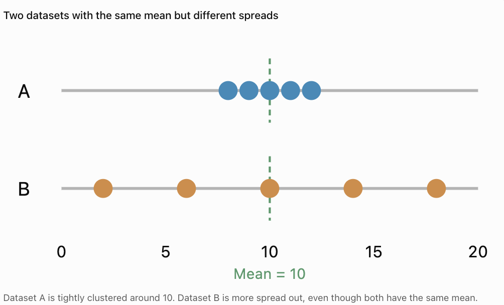
Consider:

Dataset A: 8, 9, 10, 11, 12

Dataset B: 2, 6, 10, 14, 18

Both datasets have:

Mean = 10

However, Dataset B has much greater variability.

Why Is Variability Important?

Variability helps us understand:

• Whether results are consistent.

• Whether measurements are reliable.

• How much individuals differ.

• Whether a typical value represents the whole dataset well.

• Whether unusual values may be present.

For example, two machines might produce objects with the same average mass, but one machine may produce much more consistent results.

The Range

The range is the simplest measure of spread.

It is the difference between the largest and smallest values in a dataset.

Range = Maximum value − Minimum value

Worked Example: Test Scores

Consider:

12, 15, 18, 20, 25

The maximum value is 25.

The minimum value is 12.

Range = 25 − 12

Range = 13

Interpretation

The highest score is 13 points greater than the lowest score.

The range tells us the total width of the dataset.

Finding the Range with Negative Numbers

The range can also be calculated for datasets containing negative values.

Worked Example: Temperatures

A weather station records these temperatures:

−4, −2, 1, 3, 6°C

Maximum = 6°C

Minimum = −4°C

Range = 6 − (−4)

Range = 6 + 4

Range = 10°C

Important Reminder

Subtracting a negative number is equivalent to adding its positive value.

Strengths and Limitations of the Range

Advantages

• Very easy to calculate.

• Quickly describes the total spread.

• Useful for comparing minimum and maximum measurements.

• Can be calculated for small datasets.

Limitations

• Uses only two values.

• Does not describe the distribution of the middle values.

• Can be strongly affected by outliers.

• May change dramatically when a single extreme value is added.

Example

Dataset A:

5, 6, 7, 8, 9

Range = 9 − 5 = 4

Dataset B:

5, 6, 7, 8, 100

Range = 100 − 5 = 95

Replacing one value with an extreme observation increases the range dramatically.

The range is useful, but it should not always be used alone.

Quartiles

Quartiles divide an ordered dataset into four parts.

The three quartiles are:

• First quartile (Q1): Lower quartile, associated with the 25th percentile.

• Second quartile (Q2): Median, associated with the 50th percentile.

• Third quartile (Q3): Upper quartile, associated with the 75th percentile.

Quartiles help us understand where values are concentrated.

Example

Consider the ordered dataset:

2, 4, 5, 7, 8, 10, 12, 14, 16

The median is the fifth value:

Q2 = 8

Using the median-of-halves method, exclude the overall median and divide the remaining values into two halves.

Lower half:

2, 4, 5, 7

Upper half:

10, 12, 14, 16

Find the median of each half.

Q1 = (4 + 5)/2 = 4.5

Q3 = (12 + 14)/2 = 13

Therefore:

Q1 = 4.5

Q2 = 8

Q3 = 13

Important Note About Quartile Methods

Different textbooks, calculators, and statistical software may calculate quartiles using slightly different conventions.

In these notes, we use the median-of-halves method:

• For an odd-sized dataset, exclude the overall median when forming the halves.

• For an even-sized dataset, divide the values into equal lower and upper halves.

• Find the median of each half.

Always use the method required by your course or assessment.

The Interquartile Range

The interquartile range (IQR) measures the spread of the middle 50% of a dataset.

It is calculated by subtracting the first quartile from the third quartile.

IQR = Q3 − Q1

Worked Example

Using the previous dataset:

2, 4, 5, 7, 8, 10, 12, 14, 16

We found:

Q1 = 4.5

Q3 = 13

Therefore:

IQR = 13 − 4.5

IQR = 8.5

Interpretation

The middle half of the dataset extends across an interval with width 8.5.

Unlike the range, the IQR focuses on the central portion of the data.

Finding the IQR with an Even Number of Values

Worked Example

Consider:

3, 5, 7, 8, 10, 12, 14, 18

There are eight values.

Divide the ordered dataset into two equal halves.

Lower half:

3, 5, 7, 8

Upper half:

10, 12, 14, 18

Calculate Q1:

Q1 = (5 + 7)/2 = 6

Calculate Q3:

Q3 = (12 + 14)/2 = 13

Therefore:

IQR = 13 − 6

IQR = 7

Understanding the IQR with Box Plots

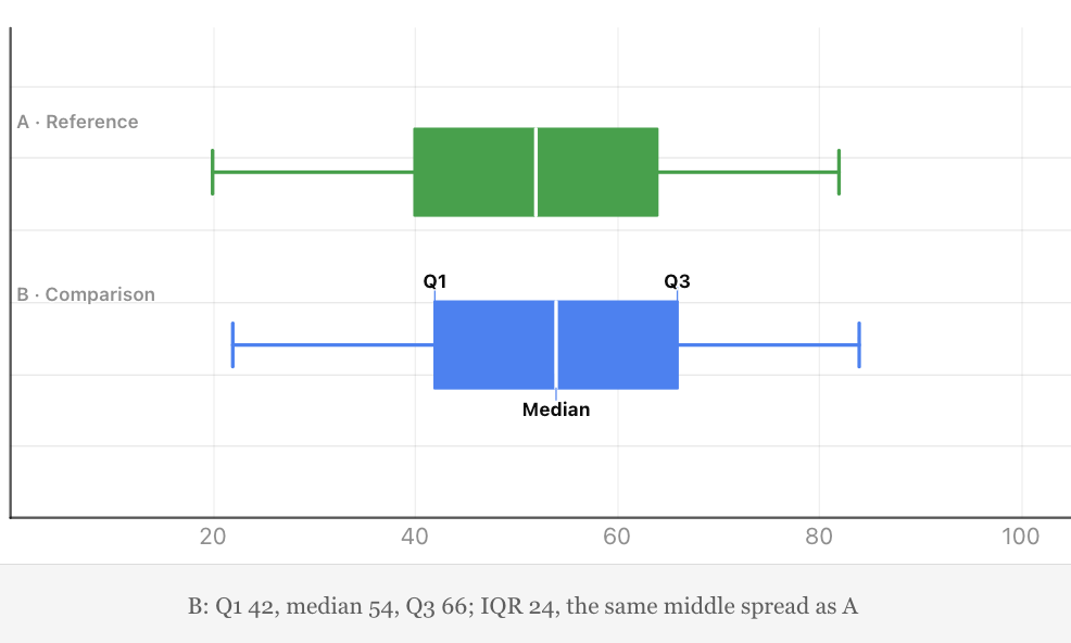
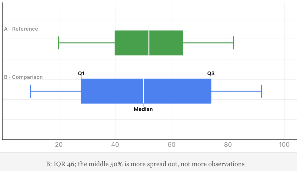
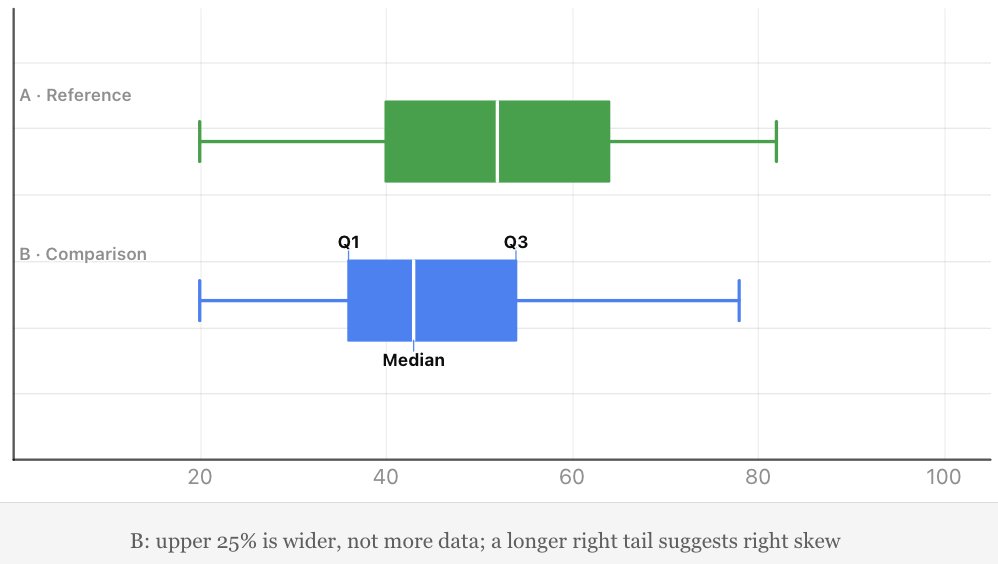
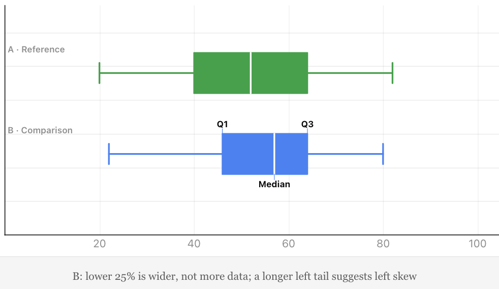
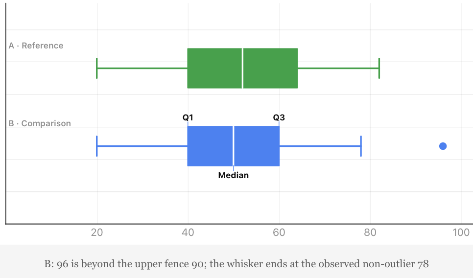
A box plot displays the distribution of numerical data using quartiles, the median, and whiskers.

The box extends from Q1 to Q3.

Its width represents the interquartile range.

A line inside the box represents the median.

In a modified box plot, whiskers usually extend to the most extreme observed values that are not classified as outliers.

Interpreting a Box Plot

A wide box indicates that the middle 50% of values has a large spread.

A narrow box indicates that the middle 50% is more closely clustered.

Box plots are particularly useful for comparing two or more datasets.

Why Is the IQR Useful?

The IQR is resistant to extreme values because it focuses on the middle half of the dataset.

For this reason, it is often preferred when data is skewed or contains outliers.

Identifying Possible Outliers Using the IQR

The IQR can help identify unusually high or low values.

A common method is the 1.5 × IQR rule.

Calculate:

Lower fence = Q1 − 1.5 × IQR

Upper fence = Q3 + 1.5 × IQR

Values outside these fences are flagged as potential outliers.

Worked Example

Consider:

2, 3, 4, 5, 6, 7, 8, 9, 30

Using the median-of-halves method:

Q1 = (3 + 4)/2 = 3.5

Q3 = (8 + 9)/2 = 8.5

IQR = 8.5 − 3.5 = 5

Calculate the fences.

Lower fence:

3.5 − 1.5(5) = −4

Upper fence:

8.5 + 1.5(5) = 16

Therefore, values below −4 or above 16 are potential outliers.

Since:

30 > 16

30 is a potential outlier.

Important Interpretation

A potential outlier is not necessarily an error.

It may represent a genuine but unusual observation.

Investigators should examine possible outliers before deciding whether to exclude them.

Variance

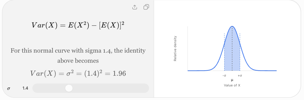
The variance measures how widely numerical values are distributed around their mean.

It is based on the squared differences between each value and the mean.

These differences are called deviations.

Why Square the Deviations?

Consider values above and below the mean.

Some deviations are positive, while others are negative.

If we simply add all deviations from the mean, the total is zero.

Squaring the deviations:

• Makes every contribution nonnegative.

• Prevents positive and negative deviations from cancelling.

• Gives greater weight to values far from the mean.

Variance is therefore a useful mathematical measure of variability.

Population Variance and Sample Variance

There are two commonly used variance formulas.

Population Variance

A population contains every member or observation in the group being studied.

Population variance is:

σ² = Σ(x − μ)²/N

Where:

• σ² = population variance

• x = individual value

• μ = population mean

• N = number of values in the population

• Σ = sum of all values

Sample Variance

A sample is a subset selected from a larger population.

Sample variance is:

s² = Σ(x − x̄)²/(n − 1)

Where:

• s² = sample variance

• x = individual value

• x̄ = sample mean

• n = number of sample observations

Why Divide by n − 1?

When we calculate variance from a sample, dividing by n − 1 rather than n corrects for the tendency of the sample's squared deviations to underestimate the population variance.

This is called Bessel's correction.

For a sample of independent observations from a population with finite variance, the n − 1 formula gives an unbiased estimator of population variance.

Which Formula Should You Use?

Use the population formula when your dataset represents the entire population of interest.

Use the sample formula when your data is a sample and you want to estimate the variability of the larger population.

Calculating Population Variance Step by Step

Worked Example

Consider the dataset:

2, 4, 6, 8, 10

Treat these five values as the entire population.

Step 1: Calculate the Mean

Mean = (2 + 4 + 6 + 8 + 10)/5

Mean = 30/5

μ = 6

Step 2: Find Each Deviation

Subtract the mean from each value.

Step 3: Add the Squared Deviations

Σ(x − μ)² = 40

Step 4: Divide by N

σ² = 40/5

Population variance = 8

Interpretation

The variance describes the average squared distance from the mean.

Because the original values have no specified units, the variance is expressed in squared data units.

If these were measurements in centimetres, the variance would be 8 cm².

Understanding Squared Deviations

The further a value is from the mean, the larger its squared deviation becomes.

For example:

• A deviation of 1 contributes 1 to the squared total.

• A deviation of 2 contributes 4.

• A deviation of 3 contributes 9.

• A deviation of 5 contributes 25.

This means extreme values can have a substantial effect on variance.

Important Observation

Variance is always greater than or equal to zero.

It equals zero only when every value in the dataset is identical.

Calculating Sample Variance

Worked Example

Suppose the values:

2, 4, 6, 8, 10

are a sample from a larger population.

The mean is:

x̄ = 6

The sum of squared deviations is:

Σ(x − x̄)² = 40

However, because the dataset is a sample:

s² = 40/(5 − 1)

s² = 40/4

Sample variance = 10

Comparison

For the same five observations:

• Population variance = 8

• Sample variance = 10

The sample variance is larger because we divide by n − 1 instead of n.

This distinction is essential when interpreting statistical results.

Standard Deviation

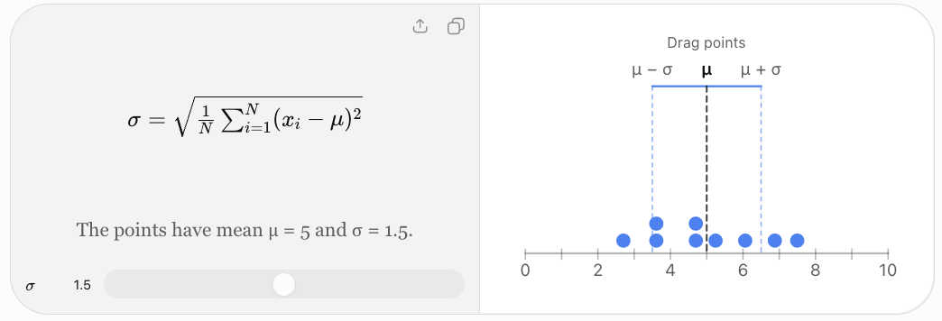
The standard deviation measures the spread of data around the mean.

It is calculated by taking the square root of the variance.

Standard deviation is especially useful because it is expressed in the same units as the original data.

Population Standard Deviation

σ = √[Σ(x − μ)²/N]

Sample Standard Deviation

s = √[Σ(x − x̄)²/(n − 1)]

Relationship Between Variance and Standard Deviation

Standard deviation = √Variance

Variance = (Standard deviation)²

Calculating Standard Deviation Step by Step

Using the dataset:

2, 4, 6, 8, 10

we previously found:

Population variance = 8

Therefore:

σ = √8

Population standard deviation ≈ 2.83

If the data represents a sample:

Sample variance = 10

Therefore:

s = √10

Sample standard deviation ≈ 3.16

Interpretation

The population standard deviation of approximately 2.83 indicates the scale of variation around the mean of 6.

Standard deviation is often described informally as a typical distance from the mean, although it is specifically the root mean square of the deviations rather than the ordinary average absolute distance.

Understanding Standard Deviation Visually

Standard deviation helps us compare how tightly or widely values cluster around their mean.

Small Standard Deviation

A small standard deviation indicates that values are relatively close to the mean.

Large Standard Deviation

A large standard deviation indicates that values are more widely spread around the mean.

Zero Standard Deviation

If all values are identical, the standard deviation is zero.

For example:

5, 5, 5, 5, 5

Mean = 5

Every deviation is zero.

Therefore:

Variance = 0

Standard deviation = 0

Comparing Two Datasets Using Standard Deviation

Consider:

Dataset A:

8, 9, 10, 11, 12

Dataset B:

2, 6, 10, 14, 18

Both have:

Mean = 10

Dataset A

Deviations:

−2, −1, 0, 1, 2

Squared deviations:

4, 1, 0, 1, 4

Sum = 10

Population variance:

σ² = 10/5 = 2

Standard deviation:

σ ≈ 1.41

Dataset B

Deviations:

−8, −4, 0, 4, 8

Squared deviations:

64, 16, 0, 16, 64

Sum = 160

Population variance:

σ² = 160/5 = 32

Standard deviation:

σ ≈ 5.66

Comparison

Dataset B has much greater variability, despite having the same mean.

Standard Deviation and the Normal Distribution

A normal distribution is a symmetrical, bell-shaped distribution.

For data that follows a normal distribution approximately:

• About 68% of observations lie within 1 standard deviation of the mean.

• About 95% lie within 2 standard deviations.

• About 99.7% lie within 3 standard deviations.

This is known as the 68–95–99.7 rule, or empirical rule.

Worked Example

Suppose examination scores are approximately normally distributed with:

Mean = 70

Standard deviation = 10

Then approximately:

• 68% of scores fall between 60 and 80.

• 95% fall between 50 and 90.

• 99.7% fall between 40 and 100.

These are approximate proportions under the assumed normal model, not guarantees for every dataset.

Important Limitation

The empirical rule should not be applied automatically to strongly skewed or irregular distributions.

Comparing Range, IQR, Variance, and Standard Deviation

When Is Each Measure Useful?

Range: When the total difference between the smallest and largest values is important.

IQR: When describing the spread of the middle half of a dataset, particularly if the data is skewed.

Variance: When performing mathematical and statistical calculations involving squared deviations.

Standard deviation: When describing variability around the mean using the original units.

Measures of Centre and Spread Together

A measure of centre describes a typical value.

A measure of spread describes how much values vary around that typical value.

Both are important.

For example, two schools may have the same mean test score but different standard deviations.

A school with a smaller standard deviation has scores that are more tightly clustered around its mean.

A school with a larger standard deviation has greater variation in student performance.

Useful Reporting Combinations

For approximately symmetrical numerical data:

Mean and standard deviation

For skewed numerical data or data with outliers:

Median and interquartile range

These are common reporting conventions, not absolute rules.

Real-World Application: Manufacturing Quality Control

A factory produces metal rods intended to have a length of 50 cm.

Two machines produce the following samples.

Machine A:

49.9, 50.0, 50.1, 50.0, 50.0

Machine B:

49.5, 50.4, 50.0, 50.6, 49.5

Both machines have a mean length of 50.0 cm.

However, Machine A produces rods with much less variation.

Machine A

Population variance:

σ² = (0.01 + 0 + 0.01 + 0 + 0)/5

= 0.004 cm²

Standard deviation:

σ ≈ 0.063 cm

Machine B

Squared deviations:

0.25, 0.16, 0, 0.36, 0.25

Sum = 1.02

Population variance:

σ² = 1.02/5 = 0.204 cm²

Standard deviation:

σ ≈ 0.452 cm

Interpretation

Machine A is more consistent.

Even though both machines have the same mean, Machine B produces rods with a much greater spread of lengths.

Real-World Application: Comparing Student Performance

Two students complete five assessments.

Student A:

78, 80, 82, 79, 81

Student B:

60, 70, 80, 90, 100

Both have:

Mean = 80

Student A

Squared deviations from 80:

4, 0, 4, 1, 1

Sum = 10

Population variance = 10/5 = 2

Population standard deviation:

σ ≈ 1.41

Student B

Squared deviations:

400, 100, 0, 100, 400

Sum = 1000

Population variance = 1000/5 = 200

Population standard deviation:

σ ≈ 14.14

Interpretation

Student A demonstrates much more consistent performance.

Student B has greater variation, including both much lower and much higher scores.

Standard deviation reveals this difference even though the mean scores are identical.

Real-World Application: Scientific Experiments

Suppose two groups of plants are grown under different conditions.

The mean plant height in both groups is 15 cm.

However:

Group A has a standard deviation of 1 cm.

Group B has a standard deviation of 4 cm.

Interpretation

Group A has more consistent plant heights.

Group B has greater variation.

This could suggest differences in environmental conditions, genetics, measurement quality, or other factors.

However, the standard deviation alone cannot establish the cause of the variability.

Scientists must consider the experimental design and other evidence.

Using Technology to Calculate Measures of Spread

Calculators and spreadsheets can calculate variance and standard deviation efficiently.

For example, in a spreadsheet with values in cells A1 through A10:

For quartiles, spreadsheet functions such as QUARTILE.INC and QUARTILE.EXC are available, but their results may differ from the median-of-halves convention used in these notes.

Important Reminder

Technology can perform calculations quickly, but students should understand what each measure represents and how it is calculated.

Common Mistakes

Confusing range with interquartile range

The range uses the maximum and minimum values. The IQR uses Q3 and Q1.

Forgetting to order data before finding quartiles

Quartiles depend on the positions of values in an ordered dataset.

Using inconsistent quartile methods

Different methods can produce different results, particularly for small datasets.

Subtracting quartiles in the wrong order

IQR = Q3 − Q1, not Q1 − Q3.

Confusing variance and standard deviation

Standard deviation is the square root of variance.

Forgetting to square deviations

Variance requires squared differences from the mean.

Forgetting to take the square root

Calculating variance is not the final step when standard deviation is required.

Using the wrong denominator

Population variance uses N. Sample variance uses n − 1.

Rounding too early

Keep sufficient decimal places during calculations and round the final answer.

Ignoring units

Variance uses squared units, while standard deviation uses the original units.

Assuming a large standard deviation always indicates poor results

A large standard deviation indicates variability, not necessarily poor quality or performance.

Ignoring outliers

Extreme observations can strongly influence range, variance, and standard deviation.

Applying the empirical rule to every distribution

The 68–95–99.7 rule applies to approximately normal distributions.

Key Terms

• Variability: Degree to which values differ within a dataset.

• Dispersion: Another term for the spread of data.

• Range: Difference between the maximum and minimum values.

• Quartile: Value used to divide ordered data into four parts.

• First Quartile (Q1): Lower quartile.

• Second Quartile (Q2): Median.

• Third Quartile (Q3): Upper quartile.

• Interquartile Range (IQR): Difference between Q3 and Q1.

• Five-Number Summary: Minimum, Q1, median, Q3, and maximum.

• Box Plot: Graph displaying quartiles, median, and whiskers.

• Outlier: Observation unusually far from other values.

• Outlier Fence: Boundary used to identify potential outliers.

• Variance: Measure based on squared deviations from the mean.

• Standard Deviation: Square root of variance.

• Deviation: Difference between a value and the mean.

• Squared Deviation: Square of a deviation.

• Population: Entire group of interest.

• Sample: Subset of a population.

• Population Variance: Variance calculated using the population mean and population size.

• Sample Variance: Variance estimate calculated using the sample mean and n − 1.

• Bessel's Correction: Use of n − 1 when calculating sample variance.

• Normal Distribution: Symmetrical bell-shaped probability distribution.

• Empirical Rule: Approximate 68–95–99.7 pattern for normal distributions.

• Consistency: Degree to which measurements or results remain similar.

• Skewness: Asymmetry in the distribution of data.

Key Takeaways

• Measures of spread describe variability in a dataset.

• The range is the difference between the largest and smallest values.

• Quartiles divide ordered data into four parts.

• The interquartile range describes the spread of the middle 50% of observations.

• The IQR is relatively resistant to extreme values.

• Variance is based on squared deviations from the mean.

• Population variance uses N in the denominator.

• Sample variance uses n − 1 in the denominator.

• Standard deviation is the square root of variance.

• Standard deviation uses the same units as the original data.

• A small standard deviation indicates relatively consistent values.

• A large standard deviation indicates greater variability.

• Extreme values can strongly influence variance and standard deviation.

• Mean and standard deviation are often reported together for approximately symmetrical data.

• Median and IQR are often preferred for skewed data.

• Measures of centre and spread should be interpreted together.

Check Your Understanding

Range

1. Find the range of 4, 7, 9, 12, 15.

2. Find the range of −5, −2, 3, 7, 10.

3. Find the range of 12, 12, 12, 12.

4. A dataset has a minimum of 8 and maximum of 37. Find the range.

Interquartile Range

Use the median-of-halves method.

5. Find the IQR of 2, 4, 6, 8, 10, 12, 14.

6. Find the IQR of 3, 5, 7, 9, 11, 13, 15, 17.

7. A dataset has Q1 = 12 and Q3 = 28. Find the IQR.

8. Explain why the IQR is less sensitive to outliers than the range.

Variance

Treat the following datasets as populations unless stated otherwise.

9. Find the population variance of 2, 4, 6.

10. Find the population variance of 5, 5, 5, 5.

11. Find the population variance of 1, 3, 5, 7.

12. A sample has values 2, 4, 6. Calculate the sample variance.

Standard Deviation

13. Find the population standard deviation of 2, 4, 6.

14. Find the population standard deviation of 5, 5, 5, 5.

15. A population has variance 25. Find its standard deviation.

16. A sample has variance 16. Find its sample standard deviation.

Interpretation

17. Which measure of spread is most strongly affected by a single extreme value: range or IQR?

18. Why is standard deviation easier to interpret than variance in terms of units?

19. Can two datasets have the same mean but different standard deviations?

20. Explain what a standard deviation of zero means.

Answers

Extended Challenge

Calculating Range and IQR

1. Find the range and IQR of 4, 6, 8, 10, 12, 14, 16.

2. Find the range and IQR of 2, 3, 5, 7, 9, 12, 15, 20.

3. Find the range and IQR of 10, 10, 12, 14, 15, 18, 20, 25, 30.

4. Construct a dataset with a range of 20 and an IQR of 5.

5. Explain how adding an extreme value might change the range and IQR.

Calculating Variance

6. Find the population variance of 3, 5, 7, 9.

7. Find the sample variance of 3, 5, 7, 9.

8. Find the population variance of 10, 12, 14, 16, 18.

9. Find the sample variance of 4, 6, 8, 10, 12.

10. Explain why sample variance is generally larger than population variance when both formulas are applied to the same nonconstant dataset.

Calculating Standard Deviation

11. Find the population standard deviation of 1, 2, 3, 4, 5.

12. Find the sample standard deviation of 1, 2, 3, 4, 5.

13. Find the population standard deviation of 20, 22, 24, 26, 28.

14. Find the sample standard deviation of 5, 10, 15, 20.

15. Explain why standard deviation cannot be negative.

Interpretation and Comparison

16. Two datasets have the same mean but standard deviations of 2 and 9. Compare their variability.

17. Explain why IQR may be preferred for income data.

18. Explain why standard deviation is useful in manufacturing.

19. Describe a situation where the range is more informative than the standard deviation.

20. Explain why measures of centre and spread should be reported together.

Final Challenge: Comparing Two Scientific Experiments

Two groups of plants are grown under different environmental conditions.

After four weeks, their heights are measured in centimetres.

Group A:

12, 13, 14, 14, 15, 15, 16, 17, 18

Group B:

6, 9, 11, 14, 15, 16, 19, 22, 27

Complete the investigation.

1. Calculate the mean height of each group.

2. Calculate the median height of each group.

3. Determine the range of each group.

4. Find Q1 and Q3 for each group using the median-of-halves method.

5. Calculate the IQR for each group.

6. Construct a five-number summary for each group.

7. Draw comparative box plots.

8. Calculate the population variance for each group, treating each group as the complete set of plants under investigation.

9. Calculate the population standard deviation for each group.

10. Compare the variability of the two groups.

11. Identify which group has more consistent plant heights.

12. Determine whether either group contains potential outliers using the 1.5 × IQR rule.

13. Explain how the range and IQR provide different information.

14. Explain how the standard deviations support your conclusions.

15. Discuss why two groups can have similar means but different spreads.

16. Suggest possible environmental factors that could influence plant growth.

17. Explain why variability is important when interpreting experimental results.

18. Identify one limitation of drawing conclusions from these datasets alone.

19. Recommend which measures of centre and spread should be reported.

20. Write a scientific conclusion comparing the two groups.

Further Investigation: Data Collection

Collect at least 20 numerical observations from a real-world situation.

Possible investigations include:

• Time taken by students to complete an activity.

• Daily temperatures over several weeks.

• Heights of plants grown under similar conditions.

• Distances travelled to school.

• Scores on a classroom assessment.

Calculate the range, quartiles, IQR, variance, and standard deviation.

Present your results in a table and construct a suitable graph.

Finally, explain what the measures reveal about the consistency and variability of the data, and discuss whether any observations appear unusual.