Measures of Centre

Introduction

When we collect data, we often want to describe the information using a single number that represents a typical or central value.

For example, imagine that a teacher records the scores of students on a mathematics quiz. Rather than examining every individual score, the teacher might calculate an average to understand how the class performed.

Similarly, a business might want to know the typical amount customers spend, or a scientist might want to determine the typical height of plants in an experiment.

These situations involve measures of centre, also called measures of central tendency.

The three most common measures of centre are:

• Mean: The sum of all values divided by the number of values.

• Median: The middle value when data is arranged in order.

• Mode: The value that occurs most frequently.

Each measure describes the centre of a dataset differently. Understanding these differences helps us select the most appropriate measure for a particular situation.

What Is a Dataset?

A dataset is a collection of values or observations gathered for analysis.

For example, consider the number of books read by eight students during a month:

2, 4, 3, 5, 4, 6, 3, 5

Each number represents one observation.

The dataset contains eight values.

We can use measures of centre to describe a typical number of books read.

Before calculating a measure of centre, it is important to understand the data.

Questions to consider include:

• How many values are there?

• Are the values numerical or categorical?

• Are any values unusually large or small?

• Are some values repeated?

• What does each value represent?

The answers help determine which measure of centre is most useful.

The Mean

The mean is calculated by adding all the values in a dataset and dividing by the number of values.

It is often called the arithmetic average.

Formula

Mean = Sum of all values ÷ Number of values

Using mathematical notation:

x̄ = Σx/n

Where:

• x̄ represents the sample mean.

• Σx represents the sum of all values.

• n represents the number of values.

The symbol Σ (sigma) means sum.

Worked Example: Quiz Scores

Five students receive the following quiz scores:

6, 8, 7, 9, 10

Find the mean.

Step 1: Add the values.

6 + 8 + 7 + 9 + 10 = 40

Step 2: Count the values.

There are 5 scores.

Step 3: Divide.

Mean = 40 ÷ 5

Mean = 8

The mean quiz score is 8.

Interpretation

The mean represents an equal-sharing value.

If the total of 40 points were distributed equally among the five students, each would have 8 points.

This does not mean every student actually scored 8.

Understanding the Mean Visually

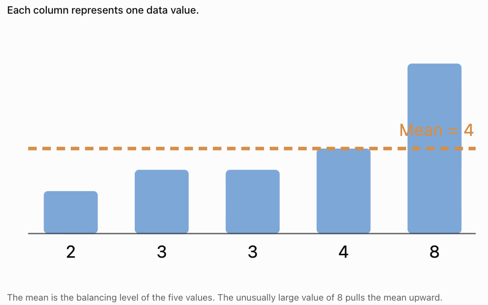
Consider the dataset:

2, 3, 3, 4, 8

Calculate:

Mean = (2 + 3 + 3 + 4 + 8)/5

= 20/5

Mean = 4

Notice that only one value is greater than 4, but that value is much larger than the others.

This demonstrates how an unusually high value can affect the mean.

Finding the Mean with Decimal Values

The mean can be calculated using whole numbers, decimals, or negative numbers.

Worked Example: Temperatures

A scientist records these temperatures in degrees Celsius:

21.5, 22.0, 23.5, 21.0, 22.5

Calculate the mean.

Add:

21.5 + 22.0 + 23.5 + 21.0 + 22.5 = 110.5

Divide by 5:

Mean = 110.5/5

Mean = 22.1°C

Important Point

The mean does not have to be one of the values in the dataset.

For example, the mean of 3 and 4 is 3.5.

Finding the Mean from a Frequency Table

Sometimes a dataset contains many repeated values.

A frequency table makes it easier to calculate the mean.

Worked Example

The following table shows the number of siblings students have.

The mean is:

Mean = Σ(f × x)/Σf

Substitute:

Mean = 19/14

Mean ≈ 1.36 siblings

Interpretation

The average number of siblings is approximately 1.36.

Although no student can have 1.36 siblings, the mean is still useful for comparing groups.

The Median

The median is the middle value of a dataset when the values are arranged in numerical order.

Unlike the mean, the median depends on the position of values rather than their total.

Finding the Median

1. Arrange the values from smallest to largest.

2. Count the number of values.

3. Find the middle position.

4. If there are two middle values, calculate their mean.

Median with an Odd Number of Values

Worked Example

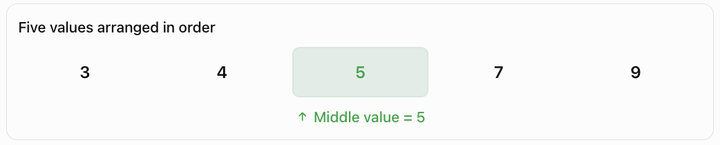
Consider:

7, 3, 9, 5, 4

Arrange in ascending order:

3, 4, 5, 7, 9

There are five values.

The middle value is the third value.

Median = 5

Median Position Formula

For an odd number of values:

Median position = (n + 1)/2

For n = 5:

Median position = (5 + 1)/2 = 3

Therefore, the median is the third value.

Median with an Even Number of Values

When a dataset contains an even number of values, there are two middle values.

The median is the mean of these two values.

Worked Example

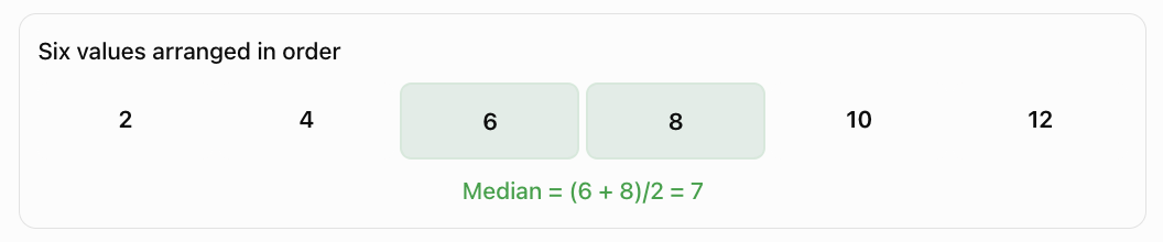
Consider:

4, 8, 2, 10, 6, 12

Arrange in ascending order:

2, 4, 6, 8, 10, 12

There are six values.

The middle values are 6 and 8.

Median = (6 + 8)/2

Median = 7

Important Observation

The median does not have to appear in the original dataset.

In this example, 7 is the median even though no value equals 7.

Why Ordering Matters

Consider:

12, 4, 8, 2, 10

A student might incorrectly select 8 because it appears in the middle of the written list.

However, the values must first be arranged in order:

2, 4, 8, 10, 12

In this particular case, the median is still 8, but this is a coincidence.

Consider instead:

12, 4, 2, 10, 8

The middle value in the original list is 2.

After sorting:

2, 4, 8, 10, 12

the median is 8.

Always arrange numerical data in order before finding the median.

The Mode

The mode is the value that occurs most frequently in a dataset.

The mode is determined by counting how many times each value appears.

Worked Example

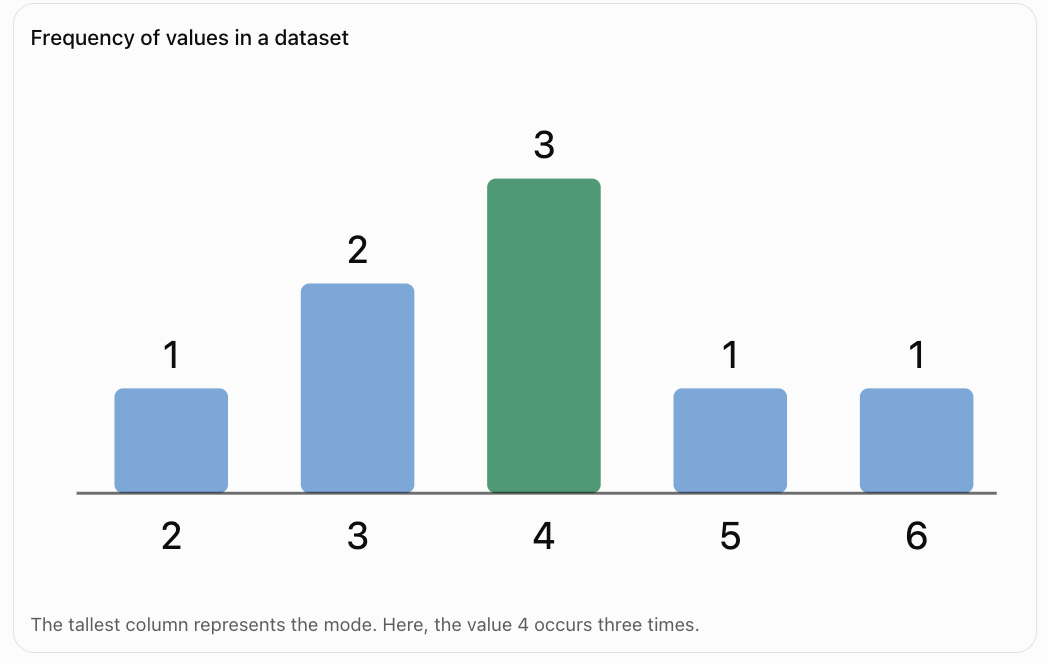
Consider:

2, 4, 3, 4, 5, 4, 6, 3

Count the frequencies:

The value 4 appears most often.

Mode = 4

Interpretation

The most common value is 4.

The mode is particularly useful when we want to identify the most frequently occurring result.

Understanding the Mode Visually

Datasets with More Than One Mode

Some datasets contain two or more values that share the highest frequency.

Bimodal Dataset

Consider:

2, 2, 3, 4, 4, 5

Both 2 and 4 appear twice.

All other values appear once.

The dataset has two modes:

Modes = 2 and 4

This is called a bimodal dataset.

Multimodal Dataset

Consider:

1, 1, 2, 2, 3, 3, 4

The values 1, 2, and 3 each appear twice.

Therefore, the dataset has three modes.

A dataset with several modes is called multimodal.

No Mode

Consider:

3, 5, 7, 9, 11

Each value appears once.

Under the usual school convention, this dataset has no mode because no value occurs more frequently than the others.

Mode with Categorical Data

Unlike the mean and median, the mode can be used with non-numerical categories.

For example, students are asked to identify their favourite fruit.

Results:

Apple, Banana, Apple, Orange, Banana, Apple, Mango

The most frequent response is Apple.

Mode = Apple

It would not make sense to calculate the mean of these categories.

The median is also not meaningful because fruit categories do not have a natural numerical order.

The mode is therefore the most appropriate measure of centre for this dataset.

Comparing Mean, Median, and Mode

Although all three measures describe the centre of data, they do so differently.

Worked Example

Consider:

3, 4, 4, 5, 9

Mean:

(3 + 4 + 4 + 5 + 9)/5 = 25/5

Mean = 5

Median:

The middle value is 4.

Median = 4

Mode:

The most frequent value is 4.

Mode = 4

Interpretation

The mean is larger than the median and mode because the high value of 9 increases the average.

The Effect of Outliers

An outlier is a value that is unusually high or low compared with the other values.

Outliers can have a significant effect on the mean.

Example: Household Incomes

Consider five annual household incomes:

$40,000, $45,000, $48,000, $50,000, $52,000

Mean:

= $235,000/5

Mean = $47,000

Median:

Median = $48,000

Now suppose a sixth household with an income of $500,000 is included.

New dataset:

$40,000, $45,000, $48,000, $50,000, $52,000, $500,000

New mean:

= $735,000/6

Mean = $122,500

New median:

= ($48,000 + $50,000)/2

Median = $49,000

Comparison

What Does This Show?

The mean increases dramatically because of the unusually high income.

The median changes only slightly.

For this dataset, the median provides a better description of a typical household income.

This is one reason median income is commonly used in economic and social statistics.

Measures of Centre and Data Distribution

The shape of a dataset can help us decide which measure of centre is most useful.

Symmetrical Distributions

A symmetrical distribution has approximately the same shape on both sides of its centre.

For a perfectly symmetric, unimodal distribution, the mean, median, and mode often coincide.

Right-Skewed Distributions

A right-skewed distribution has a longer tail toward larger values.

High values tend to pull the mean to the right.

In a typical unimodal right-skewed distribution:

Mode < Median < Mean

This ordering is common but not a universal mathematical rule.

Left-Skewed Distributions

A left-skewed distribution has a longer tail toward smaller values.

Low values tend to pull the mean to the left.

In a typical unimodal left-skewed distribution:

Mean < Median < Mode

Again, this is a common pattern rather than a guarantee for every dataset.

Choosing the Most Appropriate Measure

The best measure depends on the type of data and the purpose of the investigation.

When to Use the Mean

The mean is usually appropriate when:

• Data is numerical.

• All values should contribute to the calculation.

• There are no unusually influential outliers.

• The distribution is reasonably symmetrical.

• Further calculations require an arithmetic average.

Example: Average temperature measured during an experiment.

When to Use the Median

The median is usually appropriate when:

• The dataset contains extreme values.

• The distribution is strongly skewed.

• A typical middle value is needed.

• Data can be placed in a meaningful order.

Example: Typical household income or house price.

When to Use the Mode

The mode is usually appropriate when:

• The most common value is important.

• Data is categorical.

• We want to identify the most popular option.

• Repeated values are meaningful.

Example: Most popular shoe size in a shop.

Practical Application: Choosing Shoe Sizes

A shoe shop records the sizes of shoes sold during one day.

The shop wants to decide which size to stock most heavily.

The most appropriate measure is the mode.

Mode = Size 8

Size 8 was sold 12 times, more than any other size.

Although the mean shoe size could be calculated, it would not directly identify the most popular size.

Practical Application: Comparing Two Classes

Two classes complete the same assessment.

Interpretation

Both classes have the same median score of 8.

Class A has a slightly higher mean.

Class B has the highest possible mode of 10, but it also has several low scores.

This demonstrates why relying on only one measure of centre can be misleading.

The mean, median, and mode provide different information about the same dataset.

Real-World Application: Scientific Measurements

A scientist measures the height of six plants after four weeks.

The heights are:

12, 14, 13, 15, 14, 16 cm

Mean

Sum = 12 + 14 + 13 + 15 + 14 + 16 = 84

Mean = 84/6

Mean = 14 cm

Median

Arrange the data:

12, 13, 14, 14, 15, 16

The middle values are 14 and 14.

Median = 14 cm

Mode

The value 14 appears twice.

Mode = 14 cm

Interpretation

All three measures are equal.

This suggests that 14 cm is a reasonable central value for the measurements.

However, measures of centre alone do not describe the variation in plant heights. Measures such as range and standard deviation would provide additional information.

Comparing Datasets with the Same Mean

Two datasets can have the same mean but very different distributions.

Consider:

Dataset A:

4, 5, 6, 7, 8

Dataset B:

0, 0, 5, 10, 15

Dataset A

Mean = 30/5 = 6

Median = 6

Mode = none

Dataset B

Mean = 30/5 = 6

Median = 5

Mode = 0

Both datasets have the same mean, but the values are distributed differently.

Dataset B contains much greater variation.

This demonstrates why a measure of centre should often be considered alongside a measure of spread.

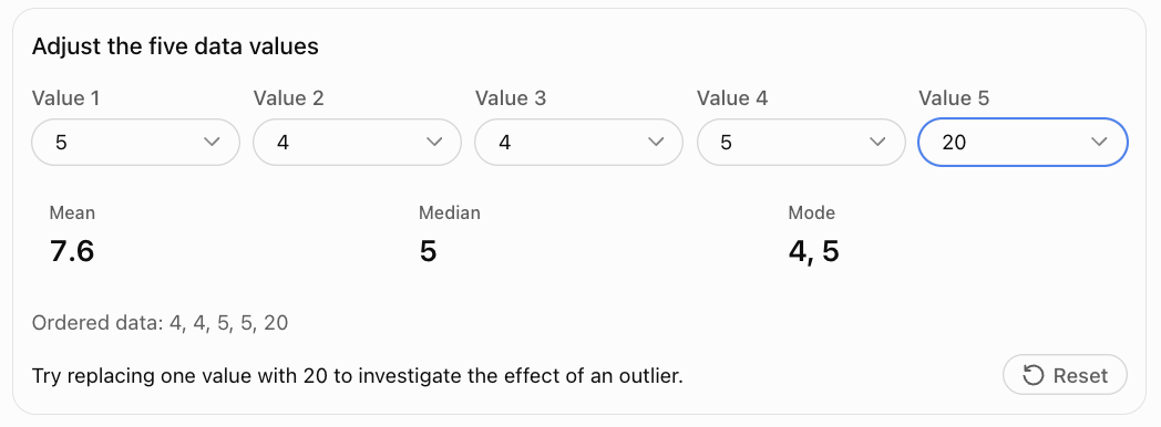
Interactive Practice: Calculate the Measures of Centre

Change the values in the dataset and observe how the mean, median, and mode respond.